Dynamic Programming Ring for Point Target Detection

Abstract

To improve the detection efficiency of a long-distance dim point target based on dynamic programming (DP), this paper proposes a multi-frame target detection algorithm based on a merit function filtering DP ring (MFF-DPR). First, to reduce the influence of noise on the pixel state estimation results, a second-order DP named the MFF-DP is proposed. The current states of pixels on an image plane are estimated by maximizing the addition of the merit functions of the previous two frames and the observation data of the current frame. In addition, to suppress the diffusion of the merit function, the sequential and reverse observation data are connected in a head-to-tail manner to form a ring structure. The MFF-DP is applied to the ring structure, and the merit function of the MFF-DPR is obtained by averaging the merit functions of the sequential and reverse MFF-DPs. Finally, the target trajectory is obtained by correlating the extreme points of the merit functions of the MFF-DPR. The simulation and analysis results show that by merely adding a ring structure, the detection probability of the traditional DP can be improved by up to 40% when detecting point targets under the SNR of 1.8. The point target detection algorithm based on the MFF-DPR can achieve significantly better performance in point target detection compared with the traditional DPs with or without a ring structure. The proposed algorithm is suitable for radars and infrared point target detection systems.

1. Introduction

As a very important technology in the field of radar or infrared systems, point target detection has been widely studied, but its development has still been limited by certain challenges. First, the point target features, such as texture and color, cannot be captured because of a far observation distance. Second, the amplitude of a point target may be less than that of its surrounding background.

The point target detection algorithms can be roughly divided into detect-before-track (DBT) [1,2,3] and track-before-detect (TBD) [4,5,6,7] algorithms, or single-frame and multi-frame target detection algorithms. When the signal-to-noise ratio (SNR) of a point target is low, the DBT algorithms can easily lose the target. In contrast, the TBD algorithms process a number of frames before making a decision on target existence. Therefore, the TBD algorithms are particularly useful when the SNR is low. Since Barniv et al. [8] first proposed the dynamic programming (DP) TBD (DP-TBD) algorithm, the DP-TBD has been the mainstream method in the field of dim point target detection because DP lowers the requirements on data storage and search range.

The DP-TBD algorithms can be roughly divided into probability density accumulation-based algorithms and energy accumulation-based algorithms according to the merit function type [9,10]. The merit functions of the probability density accumulation-based algorithms [11] require information on statistical characteristics of a signal and background noise. However, for non-cooperative targets, this prior knowledge is difficult to obtain. In contrast, the energy accumulation-based algorithms [12,13] use the gray accumulation value of each stage of a target as a merit function, which simplifies the iteration steps. For this reason, the energy density accumulation-based algorithms have a wider application scope than the probability accumulation-based algorithms. However, both types of DP-TBD algorithms have the same deficiencies, which can be summarized as follows. First, a pseudo trajectory is formed when the merit function accumulates to the nearby, strong noise. At each stage of the DP-TBD algorithms, only one optimal trajectory is retained, while other trajectories are discarded; thus, the incorrect state transition may occur in each stage due to the presence of strong noise. Second, the target merit function diffuses in each stage of the probability density or energy accumulation, which could obscure the target position. However, diffusions of the merit function cannot be completely avoided because of inherited characteristics of the DP-TBD.

To address the aforementioned problems, researchers have designed many improved algorithms for merit function. Succary et al. [14] proposed a merit function with system memory coefficient to reduce the influence of noise. However, the system memory coefficient is dependent on the SNR, and the parameter choice is challenging to detect non-cooperative targets. In recent years, the DP-TBD algorithms based on state transition constraints, including trajectory constraints [15,16,17], amplitude constraints [18], penalty function constraints [19], and multi-level thresholds [20,21], have been extensively studied. However, all of the above-mentioned improved algorithms represent first-order Markov chains. In a state-transition stage, these algorithms use only the merit function of the previous frame, which often results in a large error of pixel state estimation. Recently, the second-order DP-TBD has emerged. Unlike the first-order DP-TBD, the second-order DP-TBD uses the observation data of the previous two frames [22,23] or the subsequent frame [24,25]. However, for dim point targets, high detection accuracy is challenging to achieve when unreliable observation data are used directly for state transition decisions.

This study focuses on improving the detection efficiency of dim point targets using the DP-TBD. First, a second-order DP, named the merit function filtering DP (MFF-DP), is proposed. Unlike the traditional second-order DP, in the MFF-DP, the current states of pixels on an image plane are estimated by maximizing the addition of the merit functions of the previous two frames and the observation data of the current frame. In this way, direct involvement of the observed data in the state transition decision is avoided, thus reducing the influence of noise on the state estimation of pixels under the condition of a low SNR. Then, the symmetry of the DP merit function is determined; namely, the distribution of merit function at the target position is similar to the shape of a comet after the sequential or reverse operation of DP. The nuclei of two comets coincide, and the comet tails are symmetrical about the point target position. On this basis, a merit function diffusion suppression algorithm is designed using a DP ring (DPR); namely, this algorithm connects the sequential and reverse observation data in a head-to-tail manner to form a ring structure, calculates the merit function of the ring structure, and averages the sequential and reverse merit functions. Finally, the target trajectory is obtained by correlating the extreme points of the averaged merit function.

The remainder of this paper is organized as follows. Section 2 presents the point target model. Section 3 introduces the point target detection algorithm based on the MFF-DPR. Section 4 analyses the result of the simulation experiments to verify the effectiveness of the point target detection algorithm based on the MFF-DPR and compares the MFF-DPR with several traditional DPs with or without a ring structure. Section 5 concludes the paper.

2. Model of Point Target

In this study, it is assumed that point targets are moving relative to the radar or infrared target detection system, and the detection system obtains an observation sequence for each full scan, which is called an image, and observes a total of N images.

At time $1\le t\le N$, the observation data with coordinates of $\mathit{p}$ on an image plane $\mathit{\Omega }$ are denoted by $X_{\mathit{p}}^{\left(t\right)}$ and expressed as [15]:

$$X_{\mathit{p}}^{\left(t\right)}=\{\begin{array}{c}{A}^{\left(t\right)}+n_{\mathit{p}}^{\left(t\right)}, \mathrm{target} \mathrm{at} \mathrm{coordinates} \mathrm{of} \mathit{p}\\ n_{\mathit{p}}^{\left(t\right)}, \mathrm{no} \mathrm{target} \mathrm{at} \mathrm{coordinates} \mathrm{of} \mathit{p}\end{array},$$

(1)

where $A^{\left(t\right)}$ denotes the target amplitude, which is assumed to be a positive constant for simplicity, i.e., $A^{\left(t\right)}=A>0$; $n_{\mathit{p}}^{\left(t\right)}$ represents additive noise and obeys the zero-mean Gaussian distribution, i.e., $n_{\mathit{p}}^{\left(t\right)}~N\left(0,{\sigma }_n^2\right)$; SNR is defined as $A/{\sigma }_n$. For more details about processing a complex background, please refer to the image preprocessing presented in ref. [26].

3. MFF-DPR-Based Point Target Detection

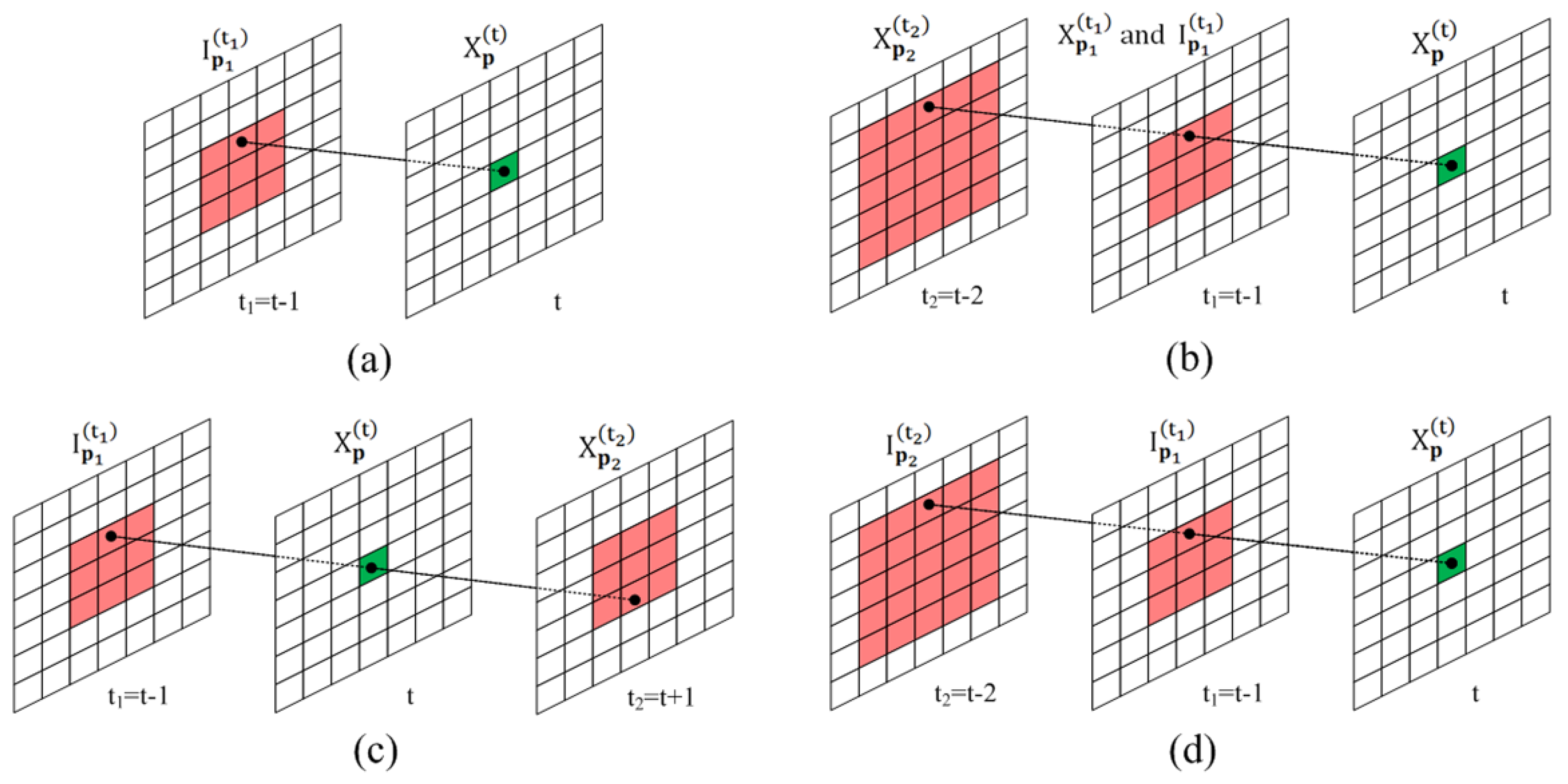
3.1. MFF-DP

According to the DP-based point target detection [14,15,16,17,18,19,20,21,22,23,24,25,26], the merit function of the DP of a pixel with coordinates of $\mathit{p}$ at time $t$ can be obtained iteratively as follow:

$$I_{\mathit{p}}^{\left(t\right)}=X_{\mathit{p}}^{\left(t\right)}+{\max }_{{\Vert \mathit{v}\Vert }_2\le v_{\max }}\left\{E_{\mathit{p},\mathit{v}}^{\left(t\right)}\right\},$$

(2)

where ${\Vert \Vert }_2$ represents the Euclidean norm, $\mathit{v}$ denotes the pixel transition velocity on the image plane, $v_{\max }$ denotes the maximum speed of the point target, and $E_{\mathit{p},\mathit{v}}^{\left(t\right)}$ represents the optimization function.

The main difference between the traditional DPs lies in $E_{\mathit{p},\mathit{v}}^{\left(t\right)}$. The optimization function of the first-order DPs [14,15,16,17,18,19,20,21] can be rewritten as $E_{\mathit{p},\mathit{v}}^{\left(t\right)}=I_{\mathit{p}-\mathit{v}}^{\left(t-1\right)}$, which means the state transition of the first-order DPs depends only on the merit function of the previous frame (Figure 1a), and the estimation error of pixel state will be large. For traditional second-order DPs [22,23,24,25], the correlation with the observation data (Figure 1b,c) is introduced to $E_{\mathit{p},\mathit{v}}^{\left(t\right)}$, which represents an improvement compared to the first-order DPs. However, for dim point targets, direct involvement of unreliable observation data in the state transition can affect the estimation of the pixel state.

To address the aforementioned problems, this study sets the optimization function $E_{\mathit{p},\mathit{v}}^{\left(t\right)}$ and depends on the merit functions of the previous two frames, as shown in Figure 1d. This avoids the direct involvement of observation data in the state transition decision as in the traditional second-order DPs, thus reducing the noise influence on the state estimation of pixels.

The trajectory of a point target in the three-dimensional space formed by an image plane and a time axis is regarded as a continuous curve, and the geometric characteristics of the trajectory are equivalent to the dynamic characteristics of the point target. When the observation time is short enough, such as three consecutive frames, the trajectory of a point target can be approximated as a straight line in a three-dimensional space. In this study, the locally linearized target trajectory in a three-dimensional space is used as a dynamic model of a point target. Thus, under the local straight-line trajectory constraints, the optimization function $E_{\mathit{p},\mathit{v}}^{\left(t\right)},$ depending on the merit functions of the previous two frames, can be defined as follows:

$$E_{\mathit{p},\mathit{v}}^{\left(t\right)}=\frac{1}{2}{w}_{\mathit{p},\mathit{v}}^{\left(t\right)}\left(I_{{\mathit{p}}_1}^{\left(t_1\right)}+I_{{\mathit{p}}_2}^{\left(t_2\right)}\right),$$

(3)

where $\frac{1}{2}$ represents the normalization coefficient of the merit function, and the velocity matching label can be expressed as:

$$w_{\mathit{p},\mathit{v}}^{\left(t\right)}=\{\begin{array}{c}1, \Vert \mathit{v}-{\mathit{v}}_{{\mathit{p}}_1}^{\left(t_1\right)}\Vert {}_{\infty }\le \frac{1}{2} \mathrm{and} \Vert \mathit{v}-{\mathit{v}}_{{\mathit{p}}_2}^{\left(t_2\right)}\Vert {}_{\infty }\le \frac{1}{2}\\ 0, \mathrm{otherwise}\end{array},$$

(4)

where ${\Vert \Vert }_{\infty }$ represents the Chebyshev norm; $\frac{1}{2}$ indicates that the estimation error of each velocity component is not larger than the minimum speed resolution of the second-order DP, i.e., $\frac{1}{2}$ pixel/frame; ${\mathit{p}}_1$ and ${\mathit{p}}_2$ denote the pixel coordinates at the previous two frames, namely, at times $t_1=t-1$ and $t_2=t-2$, respectively, $\mathit{p},{\mathit{p}}_1$, and ${\mathit{p}}_2$ satisfy the local straight-line constraint, namely, there exists a straight-line trajectory that passes through coordinates $\mathit{p},{\mathit{p}}_1$, and ${\mathit{p}}_2$ at a velocity of $\mathit{v}\in \left\{\mathit{v}|2\mathit{v}\in Z^2\right\}$. For a different coordinate $\mathit{p}$, a set $\left\{\left(\mathit{v},{\mathit{p}}_1-\mathit{p},{\mathit{p}}_2-\mathit{p}\right)|2\mathit{v}\in Z^2, {\Vert \mathit{v}\Vert }_2\le v_{\max }\right\} \mathrm{is} \mathrm{the} \mathrm{same}$. To improve the calculation efficiency, this set is used as the velocity search list of Equation (2).

Finally, the velocity corresponding to the maximum value $E_{\mathit{p},\mathit{v}}^{\left(t\right)}$ is set as a transition velocity of the pixel with coordinates of $\mathit{p}\in \mathit{\Omega }$ at the current time $t$, i.e.,

$${\mathit{v}}_{\mathit{p}}^{\left(t\right)}={\mathrm{argmax}}_{{\Vert \mathit{v}\Vert }_2\le v_{\max }}\left\{E_{\mathit{p},\mathit{v}}^{\left(t\right)}\right\}.$$

(5)

The second-order DP proposed in this paper represents the mean of the merit functions of the previous two frames under the straight-line trajectory constraints. Considering the difference from the traditional DPs, the above algorithm is named the merit function filtering DP (MFF-DP).

3.2. MFF-DPR

The MFF-DP shares the same drawback with the traditional DPs. As the merit function diffuses (Figure 2), the target will be drowned in the diffused bright spots, which complicates target detection. Therefore, suppressing the merit function diffusion of DP is of great significance to a point target detection algorithm.

The study on the diffusion of the merit function of the DP-TBD has shown that the distribution of the merit function at the target position is similar to the shape of a comet after the sequential or reverse operation. The nuclei of two comets coincide, and the comet tails are symmetrical about the position of a point target, as shown in Figure 2a,b,d,e. In this paper, the above property is named as the time reversal symmetry of DP. If the merit functions accumulated in sequential and reverse orders are superimposed together (Figure 2c,f), the merit function of a point target is enhanced after superimposition due to the coincidence of comet nuclei, and other areas are well suppressed. Consequently, the target position becomes more pronounced and is consistent with the extreme value position of the merit function on the local image plane.

Based on the time reversal symmetry of the DPs, this paper connects the sequential and reverse observation data head to tail to form a ring structure and employs the DP to update the pixel state on the ring structure, as shown in Figure 3, thus obtaining a DP ring (DPR) algorithm. Taking the MFF-DP as an example, this paper provides the steps of the corresponding DPR algorithm, i.e., the MFF-DPR algorithm, as shown in Algorithm 1. The same approach can be applied to other DPs.

To distinguish the sequential MFF-DP, reverse MFF-DP and MFF-DPR, “+”, “−”, and “*” are used in time expressions, respectively.

Algorithm 1 MFF-DPR

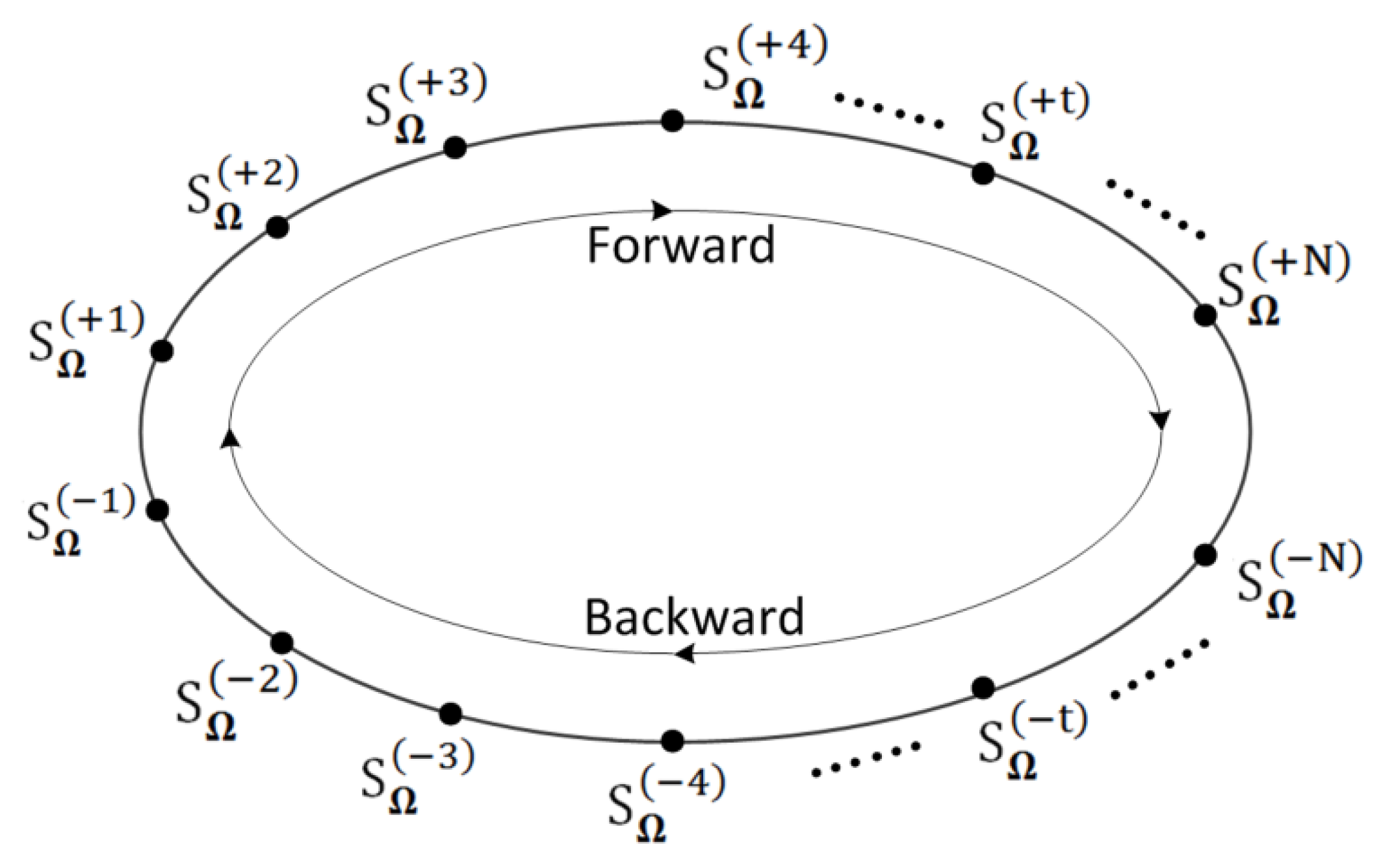
Input: Assume the upper limit of the point target motion speed is $v_{\max }$, the sequence length is $N$, the iteration counter is $k=1$, and the present time $t=+3$. Output: The merit function of the MFF-DPR $I_{\mathit{\Omega }}^{\left(\ast t\right)}$. Step 1: Pixel state updating.    Pixel state $S_{\mathit{\Omega }}^{\left(t\right)}=\left\{\left(I_{\mathit{p}}^{\left(t\right)},{\mathit{v}}_{\mathit{p}}^{\left(t\right)}\right)|\mathit{p}\in \mathit{\Omega }\right\}$ is updated weekly along the data ring, as shown in Figure 3.    If $t=+3$ or $+4$, due to the lack of prior information on the velocity, according to Equations (2), (3) and (5), the state estimation is performed in the following way: $$\{\begin{array}{c}{\mathit{v}}_{\mathit{p}}^{\left(t\right)}={\mathrm{argmax}}_{{\Vert \mathit{v}\Vert }_2\le v_{\max }}\left\{X_{{\mathit{p}}_1}^{\left(t_1\right)}+X_{{\mathit{p}}_2}^{\left(t_2\right)}\right\}\\ I_{\mathit{p}}^{\left(t\right)}=X_{\mathit{p}}^{\left(t\right)}+\frac{1}{2}{\max }_{{\Vert \mathit{v}\Vert }_2\le v_{\max }}\left\{X_{{\mathit{p}}_1}^{\left(t_1\right)}+X_{{\mathit{p}}_2}^{\left(t_2\right)}\right\}\end{array},$$ (6) where ${\mathit{p}}_1$ and ${\mathit{p}}_2$ denote the pixel coordinates at the previous two frames, namely, at times $t_1=t-1$ and $t_2=t-2$, respectively; $\mathit{p},{\mathit{p}}_1$, and ${\mathit{p}}_2$ satisfy the straight-line constraint.    If $t=+\left(N+1\right)$, let $t=-\left(N-1\right)$, and the first two states of the reverse MFF-DP are initialized in the following way: $$\{\begin{array}{c}{\mathit{v}}_{\mathit{\Omega }}^{\left(-N\right)}=-{\mathit{v}}_{\mathit{\Omega }}^{\left(+N\right)},{\mathit{v}}_{\mathit{\Omega }}^{\left(-\left(N-1\right)\right)}=-{\mathit{v}}_{\mathit{\Omega }}^{\left(+\left(N-1\right)\right)}\\ I_{\mathit{\Omega }}^{\left(-N\right)}=I_{\mathit{\Omega }}^{\left(+N\right)},I_{\mathit{\Omega }}^{\left(-\left(N-1\right)\right)}=I_{\mathit{\Omega }}^{\left(+\left(N-1\right)\right)}\end{array}.$$ (7)    If $t=0$, let $t=+2$, the first two states of the sequential MFF-DP are defined in the following way: $$\{\begin{array}{c}{\mathit{v}}_{\mathit{\Omega }}^{\left(+1\right)}=-{\mathit{v}}_{\mathit{\Omega }}^{\left(-1\right)},{\mathit{v}}_{\mathit{\Omega }}^{\left(+2\right)}=-{\mathit{v}}_{\mathit{\Omega }}^{\left(-2\right)}\\ I_{\mathit{\Omega }}^{\left(+1\right)}=I_{\mathit{\Omega }}^{\left(-1\right)},I_{\mathit{\Omega }}^{\left(+2\right)}=I_{\mathit{\Omega }}^{\left(-2\right)}\end{array}.$$ (8)    Otherwise, the pixel state $S_{\mathit{\Omega }}^{\left(t\right)}$ is updated in the way of iteration using Equations (2)–(5).    The iteration counter increased by one, i.e., $k=k+1$; if $k\le 2N$,$t=t+1$, the algorithm returns to the Step 1 of pixel state updating; otherwise, it proceeds to the Step 2 of MFF-DPR merit function derivation. Step 2: MFF-DPR merit function derivation.    The merit function of the MFF-DPR $I_{\mathit{\Omega }}^{\left(\ast t\right)}$ can be obtained by averaging merit functions of the sequential and reverse MFF-DPs at the same time, which can be expressed as follows: $$I_{\mathit{\Omega }}^{\left(\ast t\right)}=\frac{1}{2}\left(I_{\mathit{\Omega }}^{\left(+t\right)}+I_{\mathit{\Omega }}^{\left(-t\right)}\right), 1\le t\le N.$$ (9)

3.3. Multi-Target Detection

After the energy accumulation of point targets based on the MFF-DPR, the point targets can be detected by correlating the extreme points of the merit function of the MFF-DPR $I_{\mathit{\Omega }}^{\left(\ast t\right)}$. However, when there are multiple targets in the field of view, trajectories of different point targets can intersect, causing the merit functions of multiple point targets to interfere with each other, so a wrong correlation of target identifications can easily occur. To address this problem, this paper uses the target coordinates extracted in multiple iterations to detect the target trajectories one by one, and reduces the target identification error through trajectory regularization, as shown in Figure 4.

The steps of the multi-target detection algorithm based on the MFF-DPR are given in Algorithm 2. The same approach can be applied to other multi-target detection algorithms based on the DP/DPR.

Algorithm 2 Multi-Target Detection

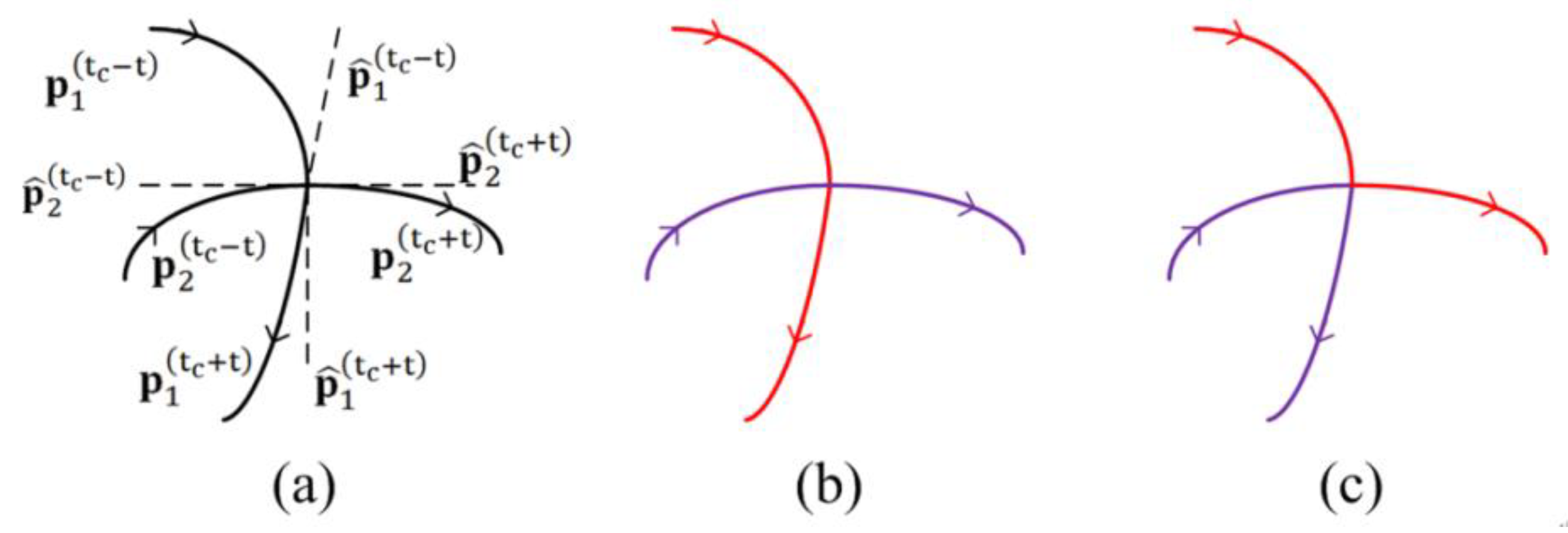
Input: Set the number of iterations to be equal to the target number, i.e., $L=N_{\mathrm{tar}}$; the sequence length is $N$, and the iteration counter is set to $l=1$. Output: The multi-target trajectories $\left\{{\mathit{p}}_i^{\left(t\right)}|1\le i\le N_{\mathrm{tar}},1\le t\le N\right\}$. Step 1: Energy accumulation.    Run Algorithm 1 for the merit functions of the MFF-DPR of the $l\mathrm{th}$ iteration $\left\{I_{\mathit{\Omega }}^{\left(l,\ast t\right)}\right|1\le t\le N\}$. Step 2: Merit function maximum value coordinates extraction.    The coordinates corresponding to the maximum value of the merit function of the MFF-DPR at time $t$ during the $l\mathrm{th}$ iteration can be expressed as: $${\mathit{p}}^{\left(l,\ast t\right)}={\mathrm{argmax}}_{\mathit{p}\in \mathit{\Omega }}\left\{I_{\mathit{p}}^{\left(l,\ast t\right)}\right\}.$$ (10) Step 3: Trajectory detection.    To prevent the same trajectory is detected multiple times, in this study, target trajectories are detected one by one. Step (3) outputs one trajectory at a time, and the trajectory can be generated by correlating the coordinate set $\left\{{\mathit{p}}^{\left(l,\ast t\right)}|1\le t\le N\right\}$. The specific steps are as follows:    Step 3.1: Trajectory initialization.    For the maximum value coordinate without matching the previous frame, a search window with a size of $\left(2v_{\max }+1\right)\times \left(2v_{\max }+1\right)$ is set by centering it on this coordinate point. If there exists a maximum value coordinate within the search window, a new trajectory is established, and the tracking counter is set to two; then, a $3\times 3$ search window of the next frame centered on the predicted point is set, and the prediction counter is set to zero; otherwise, the maximum value coordinate of the previous frame is considered a noise coordinate and thus is deleted.    Step 3.2: Trajectory generation.    For the established trajectory, if there is a maximum value coordinate in the search window, the tracking counter is increased by one. Then, the trajectory is extended to the matching point, a $3\times 3$ search window of the next frame centered on the predicted point is set, and the prediction counter is set to zero. If no matching point is found, the trajectory is extended to the prediction point, the search window of the next frame centered on the predicted point is set, the size of the search window is increased by 2 pixels, and the prediction counter is increased by one. If the prediction counter is greater than five, the point target corresponding to the trajectory has been lost, and the current trajectory updating process is terminated. In this process, the least squares linear prediction algorithm with five consecutive frames is used for coordinate prediction.    Step 3.3: The highest-score trajectory selection.    The trajectory coordinates are scored as follows: invalid coordinates as “0”, initial coordinates as “1”, prediction coordinates as “2”, and matching coordinates as “3”. After batch processing, as shown in Steps (3.1) and (3.2), the coordinate scores of each trajectory are added to the trajectory score. The trajectory’s coordinates ${\mathit{p}}_{\mathrm{traj}}^{\left(l,t\right)}$ and trajectory score $S_{\mathrm{traj}}^{\left(l,t\right)}$ corresponding to the highest-score trajectory are output.    The iteration counter is increased by one, i.e., $l=l+1$. If $l\le L$, the algorithm goes to Step 4; otherwise, it goes to Step 5. Step 4: Updating observation data.    To prevent the same trajectory is detected multiple times, once the trajectory is detected, the corresponding pixels in the observation data are replaced by adjacent background pixels.    Define the updating area ${\mathit{\Omega }}_{\mathrm{traj}}^{\left(l,t\right)}=\left\{\mathit{q}\right|\Vert \mathit{q}-{\mathit{p}}_{\mathrm{traj}}^{\left(l,t\right)}{\Vert }_{\infty }\le 1\}$, and perform $3\times 3$ median filtering filling on it as follows: $$X_{\mathit{p}}^{\left(t\right)}=\mathrm{med}\left\{X_{\mathit{q}}^{\left(t\right)}|{\Vert \mathit{p}-\mathit{q}\Vert }_{\infty }\le 1\right\},\mathit{p}\in {\mathit{\Omega }}_{\mathrm{traj}}^{\left(l,t\right)},1\le t\le N,$$ (11) where ${\Vert \Vert }_{\infty }$ represents the Chebyshev norm, and $\mathrm{med}\{ \}$ stands for the operation of calculating the median of the set elements; go to Step 1. Step 5: Trajectory regularization.    In theory, complete target trajectories can be extracted from observation data by performing Steps 1–4. However, target identification errors caused by trajectory intersection could arise, as shown in Figure 4c. To mitigate the target identification errors, this paper proposes an algorithm on any two trajectories as follows:    Assume that the trajectory coordinate sets of two trajectories are denoted by $\left\{{\mathit{p}}_1^{\left(t\right)}|1\le t\le N\right\}$ and $\left\{{\mathit{p}}_2^{\left(t\right)}|1\le t\le N\right\}$; then, if $$\min \left\{{\Vert {\mathit{p}}_1^{\left(t\right)}-{\mathit{p}}_2^{\left(t\right)}\Vert }_2|1\le t\le N\right\}\ge 5,$$ (12) then, the two trajectories do not intersect, and the trajectory regularization of the two trajectories terminates; otherwise, the time of intersecting of the two trajectories is obtained by: $$t_c={\mathrm{argmin}}_{1\le t\le N}\left\{{\Vert {\mathit{p}}_1^{\left(t\right)}-{\mathit{p}}_2^{\left(t\right)}\Vert }_2\right\},$$ (13) and trajectory regularization is performed as follows:    Suppose ${\mathit{p}}_1^{\left(t_c-t\right)}$,${\mathit{p}}_1^{\left(t_c+t\right)}$,${\mathit{p}}_2^{\left(t_c-t\right)}$, and ${\mathit{p}}_2^{\left(t_c+t\right)}$ denote local trajectories at time $t_c$, and ${\widehat{\mathit{p}}}_1^{\left(t_c-t\right)}$,${\widehat{\mathit{p}}}_1^{\left(t_c+t\right)}$,${\widehat{\mathit{p}}}_2^{\left(t_c-t\right)}$ and ${\widehat{\mathit{p}}}_2^{\left(t_c+t\right)}$ are the predicted trajectories obtained by the straight-line fitting of ${\mathit{p}}_1^{\left(t_c+t\right)}$,${\mathit{p}}_1^{\left(t_c-t\right)}$,${\mathit{p}}_2^{\left(t_c+t\right)}, \mathrm{and} {\mathit{p}}_2^{\left(t_c-t\right)}$, respectively, as shown in Figure 4a; where, $1\le t\le T_L$. The fitting errors of the two types of trajectories can be calculated by: $$\{\begin{array}{c}{E}_1={{\displaystyle \sum }}_{1\le t\le T_L}{\Vert \mathsf{\Delta }{\mathit{p}}_{11}^{\left(-t\right)}\Vert }_2^2+{\Vert \mathsf{\Delta }{\mathit{p}}_{22}^{\left(-t\right)}\Vert }_2^2+{\Vert \mathsf{\Delta }{\mathit{p}}_{11}^{\left(+t\right)}\Vert }_2^2+{\Vert \mathsf{\Delta }{\mathit{p}}_{22}^{\left(+t\right)}\Vert }_2^2\\ E_2={{\displaystyle \sum }}_{1\le t\le T_L}{\Vert \mathsf{\Delta }{\mathit{p}}_{12}^{\left(-t\right)}\Vert }_2^2+{\Vert \mathsf{\Delta }{\mathit{p}}_{21}^{\left(-t\right)}\Vert }_2^2+{\Vert \mathsf{\Delta }{\mathit{p}}_{12}^{\left(+t\right)}\Vert }_2^2+{\Vert \mathsf{\Delta }{\mathit{p}}_{21}^{\left(+t\right)}\Vert }_2^2\end{array},$$ (14) where $\mathsf{\Delta }{\mathit{p}}_{ij}^{\left(\pm t\right)}={\mathit{p}}_i^{\left(t_c\pm t\right)}-{\widehat{\mathit{p}}}_j^{\left(t_c\pm t\right)}$, and $T_L=10$ based on experience.    If $E_1<E_2$, the trajectory correlation is performed using the method shown in Figure 4b; otherwise, the method shown in Figure 4c is employed.

The probability of target identification errors can be reduced by regularization but cannot be eliminated completely. For instance, if two trajectories that intersect at time $t_c$ have the same three-dimensional tangent vector, errors of the two types of trajectory fitting methods will be very close ($E_1\approx E_2$), making it impossible to perform the trajectory correlation in the absence of other prior information about the target.

4. Simulations and Analysis

The DPR-based small target detection algorithm was simulated and verified using the MATLAB software running on a computer with a processor i5-2400CPU at 3.10 GHz and 3.40-GB memory. The simulation experiment consisted of two parts: detection of a single target and detection of multiple targets. The MFF-DP was compared with the DP algorithm proposed by Johnston [15], which represents classic first-order DP (CFO-DP) algorithm and the DP with backtracking proposed in Ref. [25], which represents the classic second-order DP (CSO-DP) algorithm. The DPR versions of the three algorithms, i.e., MFF-DPR, CFO-DPR, and CSO-DPR, were also compared. The comparison algorithms were set to optimal parameters, and the CSO-DP/DPR algorithm used the trajectory constraint-based optimization state transition model described in Section 3.1.

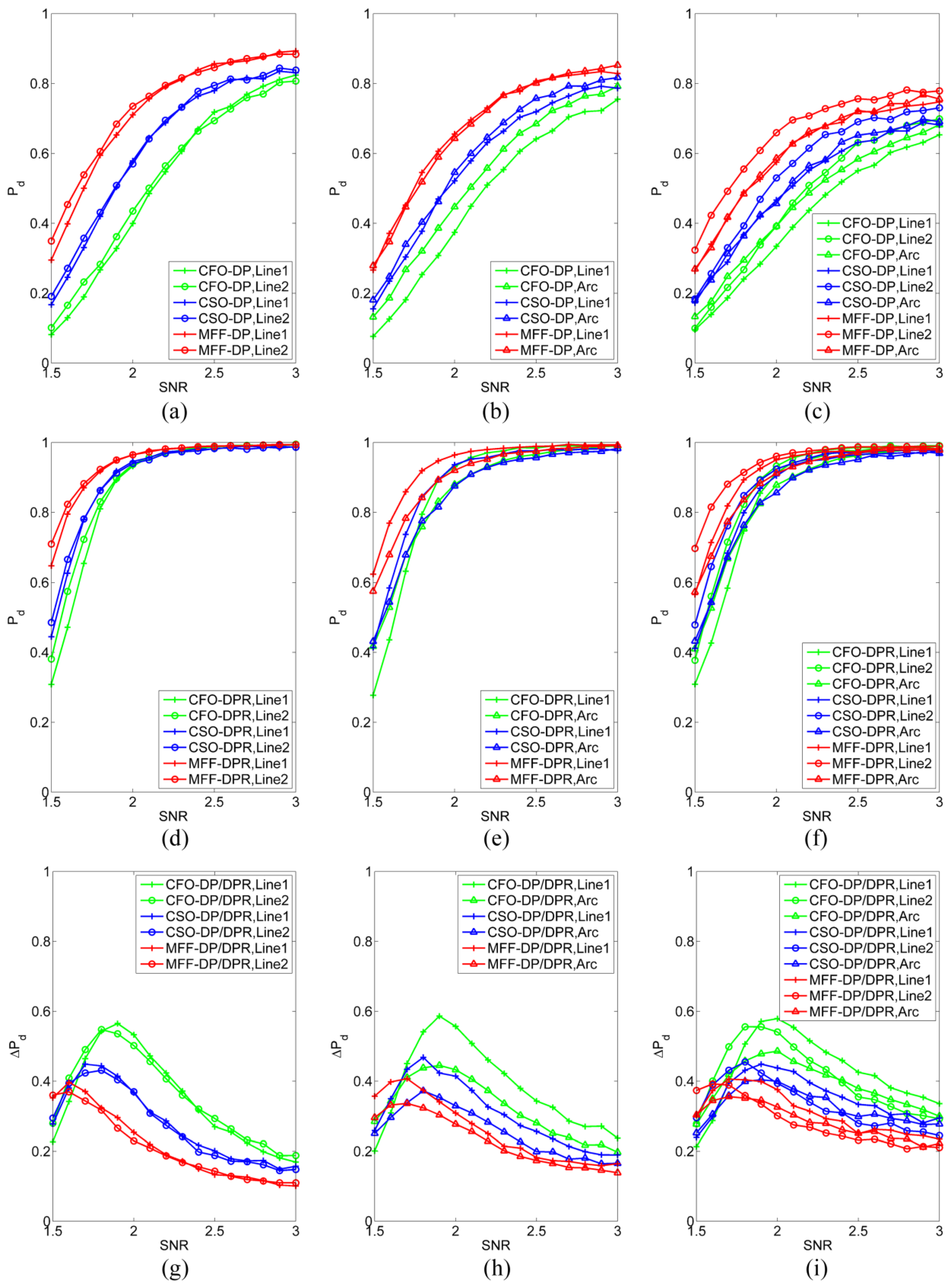
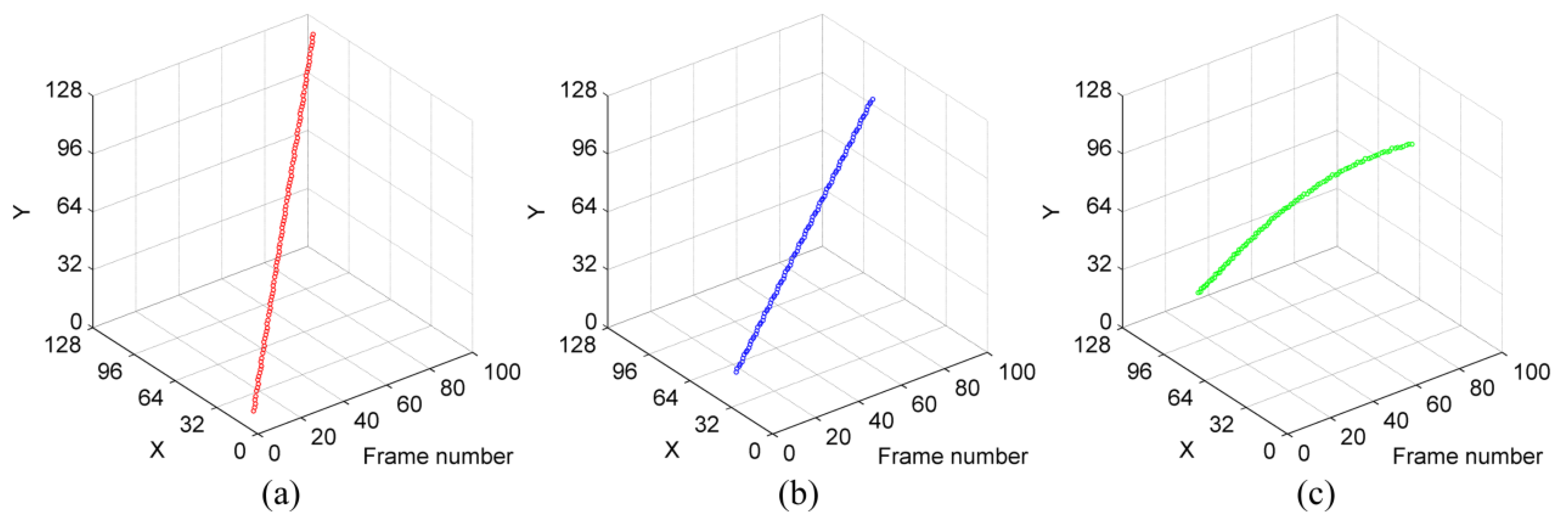
4.1. Single-Target Detection Test

The images used in the simulation had a size of $128\times 128$ pixels; the maximum sequence length was 100, and the background noise was $n_{\mathit{p}}^{\left(t\right)}~N\left(0,1\right)$. Three types of trajectories were tested in the single-point target detection experiment, as shown in Figure 5. The SNRs of the point targets on each trajectory were in the range of 1.5–3.0. For each group of test data, 1000 rounds of simulations were conducted, and the average detection probability was calculated by:

$$P_d=\frac{\mathrm{Number} \mathrm{of} \mathrm{correctly} \mathrm{detected} \mathrm{targets}}{\mathrm{Total} \mathrm{number} \mathrm{of} \mathrm{real} \mathrm{targets}}$$

(15)

According to the point target detection algorithm described in Section 3.3, only one round of the DP/DPR signal accumulation was needed, and only a single-pixel coordinate needed to be extracted from a single image frame. The single-point target detection process was simplified as follows.

Suppose that the maximum value of the merit function $I_{\mathit{p}}^{\left(t\right)}$ at time $t$ corresponds to the coordinate of ${\mathit{p}}_c^{\left(t\right)}={\mathrm{argmax}}_{\mathit{p}\in \mathit{\Omega }}\left\{I_{\mathit{p}}^{\left(t\right)}\right\}$, and the theoretical coordinate of the point target is ${\mathit{p}}_r^{\left(t\right)}$, if ${\Vert {\mathit{p}}_c^{\left(t\right)}-{\mathit{p}}_r^{\left(t\right)}\Vert }_{\infty }\le 1$; then, it can be deemed that the point target has been detected at the time $t$.

To compare the performances of the DP and DPR, we used a concept of detection probability increment $\mathsf{\Delta }{P}_d$, which is defined as the difference in the detection probability value between the DPR and DP ($\mathsf{\Delta }{P}_d=P_{\mathrm{d},\mathrm{DPR}}-P_{\mathrm{d},\mathrm{DP}}$).

The performances of the MFF-DP, CFO-DP, and CSO-DP algorithms in detecting a single-point target were tested at first. In the three test cases, different numbers of image frames (20, 50, and 100) were used. The upper limit of the motion speed of a target was $v_{\max }=2\mathrm{pixel}/\mathrm{frame}$ $\mathrm{in} \mathrm{test} \mathrm{case} 1$, and $1 \mathrm{pixel}/\mathrm{frame}$ in test cases 2 and 3.

With the increase in SNR or the number of data frames, the detection performances of the three algorithms improved gradually. The results in Figure 6a,b show that the smaller the value of $v_{\max }$ was, the smaller the number of state transition searches, the lower the noise interference, and the higher the detection probability was.

The results show that the state transition model of the MFF-DP reduced the target state estimation error compared with the first-order DP and also avoided the direct involvement of the observation data in the state transition decision process, which is one of the main drawbacks of the traditional second-order DP, thus reducing the influence of noise on the point target state estimation. When $SNR<2.0$, the detection performance of the MFF-DP was superior to that of the traditional DPs. The descending order of the algorithms regarding the detection performance was as follows: MFF-DP, CSO-DP, and CFO-DP. Particularly, at $SNR=1.5$, the highest detection probability of the CFO-DP algorithm was only about 20%, which was far lower than that of the MFF-DP algorithm, which was 45%. The highest detection probability of the CSO-DP algorithm was between those of the two above-mentioned algorithms, and it was about 30%. Above the level of 2.0, the increase in SNR would lead to higher credibility of the original data of a point target, as well as higher efficiency of point target signal accumulation. Particularly, when the number of data frames was very small ($N$ = 20), the detection probability of the CSO-DP algorithm was higher than that of the MFF-DP algorithm, as shown in Figure 6a.

Next, the performances of the MFF-DPR, CFO-DPR, and CSO-DPR algorithms in detecting a single-point target were tested. When $SNR<2.0$, the DPR algorithms achieved significantly higher detection performances than their DP counterparts, as shown in Figure 6g–i. The performances of the DPR algorithms regarding the detection probability $P_d$ (Figure 6d–f) can be mainly attributed to the state transition model, target motion speed limit, and the number of image data frames.

Similar to the MFF-DP algorithm, the MFF-DPR algorithm had the best detection performance when $SNR<2.0$. However, under the conditions of $SNR>2.0$, the detection probability of the CSO-DPR algorithm could be higher than that of the MFF-DPR algorithm, especially when the number of data frames is small ($N$ = 20), as shown in Figure 6d.

Since the number of single-step state searches determines the upper detection performance limit of the DP/DPR, and this number is approximately proportional to the square of the motion speed limit $v_{\max }$ of a target, the detection performance will be low if $v_{\max }$ is high. When $v_{\max }=2 \mathrm{pixel}/\mathrm{frame}$ and $SNR=1.5$, even the MFF-DPR algorithm, which is currently the algorithm with the highest performance, could achieve only a detection probability $P_d$ of less than 40%, as shown in Figure 6d. For the long-distance point target detection, it is necessary to eliminate the influence of the detection platform motion or to improve the image frame rate. The motion speeds of the straight-line and curve trajectories were both $v_2=1 \mathrm{pixel}/ \mathrm{frame}$. However, compared with the straight-line trajectory, the prediction error of the curve trajectory was larger; therefore, the merit function of the curve trajectory diffused faster. In addition, both the detection probability $P_d$ (Figure 6f) and the detection probability increment $\mathsf{\Delta }{P}_d$ (Figure 6i) of the curve trajectories were lower than those of the straight-line trajectories (Figure 6e,h).

As the number of image frames increased, the peak value of $\mathsf{\Delta }{P}_d$ tended to move toward the low end of SNR, as shown in Figure 6g–i. However, with the increase in the number of image frames, the growth rate of detection probability gradually decreased, as shown in Figure 6d–f, indicating that blindly increasing the number of image frames could not significantly improve the detection performance. Therefore, it is necessary to select an appropriate number of image frames according to the target SNR so as to reduce unnecessary calculation while ensuring a reasonably high detection probability.

Finally, the single-frame processing time was used as an evaluation measure of the operating efficiency of the algorithms, and the obtained results are given in

Table 1. Comparison of the computational efficiencies of the DP/DPR algorithms in single-target detection.

		CFO-DP/DPR	CSO-DP/DPR	MFF-DP/DPR
Number of single-step state searches	$v_{\max }=1\mathrm{pixel}/\mathrm{frame}$	9	49	49
	$v_{\max }=2\mathrm{pixel}/\mathrm{frame}$	25	165	165
Single-frame processing time (ms)	$v_{\max }=1\mathrm{pixel}/\mathrm{frame}$	15/29	57/117	75/155
	$v_{\max }=2\mathrm{pixel}/\mathrm{frame}$	32/63	165/343	227/449

. The main affecting factor of the single-frame processing time was the number of single-step state searches, i.e., the length of the velocity search list. As the CFO-DP and DPR are the first-order algorithms, they require fewer single-step state searches and have higher operating efficiency than the CSO-DP and DPR algorithms, as well as the MFF-DP and DPR algorithms. The data structure of DPR defines that DPR algorithms require about twice longer processing time than the corresponding DP algorithms.

Among the six algorithms, the MFF-DPR algorithm exhibits good detection performance but requires a long processing time. When the image size was $128\times 128$ pixels and $v_{\max }=2 \mathrm{pixel}/\mathrm{frame}$, the MFF-DPR algorithm needed about 0.5 s to process a single frame, which made it difficult to realize real-time processing. Thus, a balance must be stricken between the operating efficiency and detection performance in real-world applications.

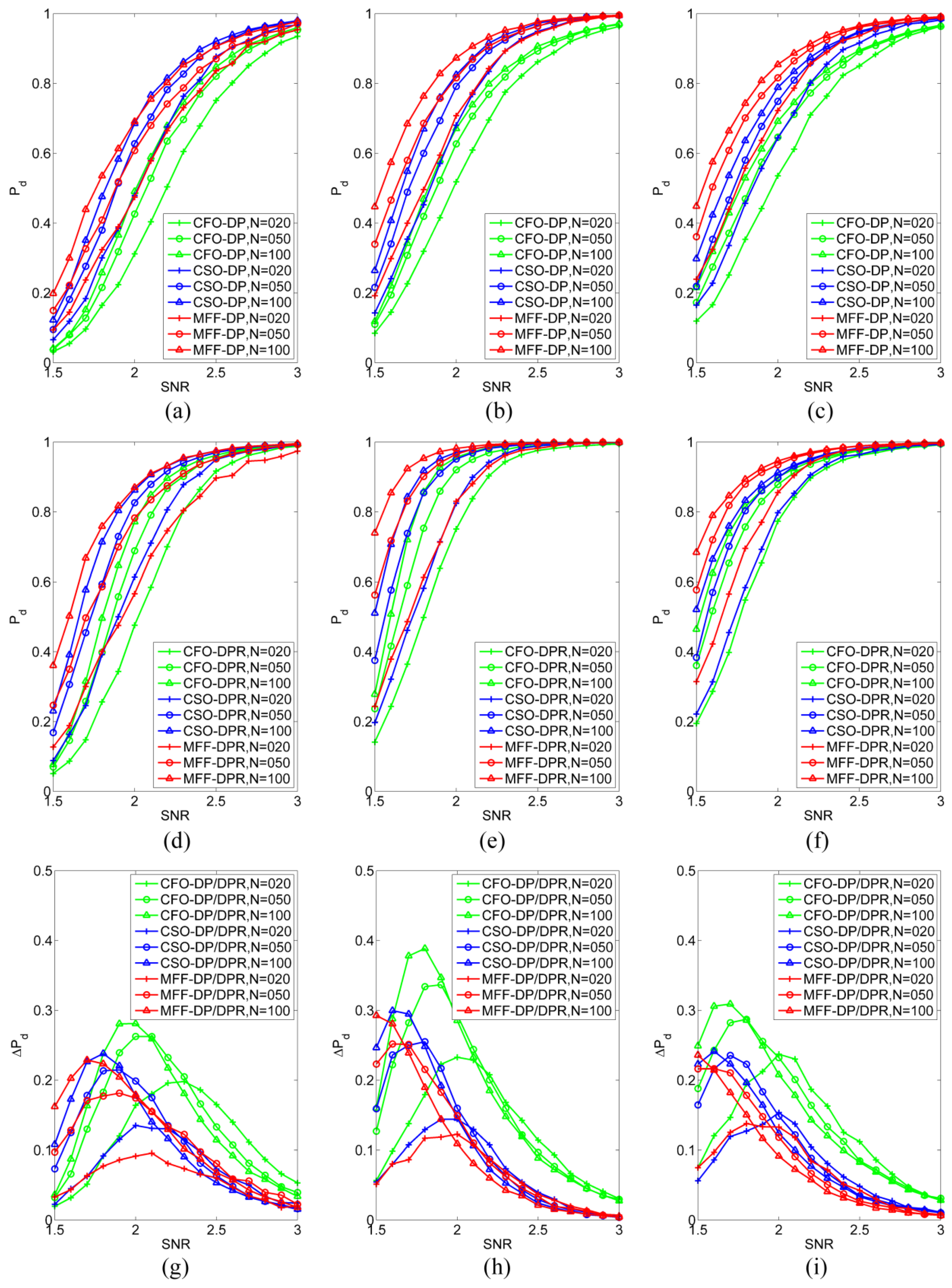
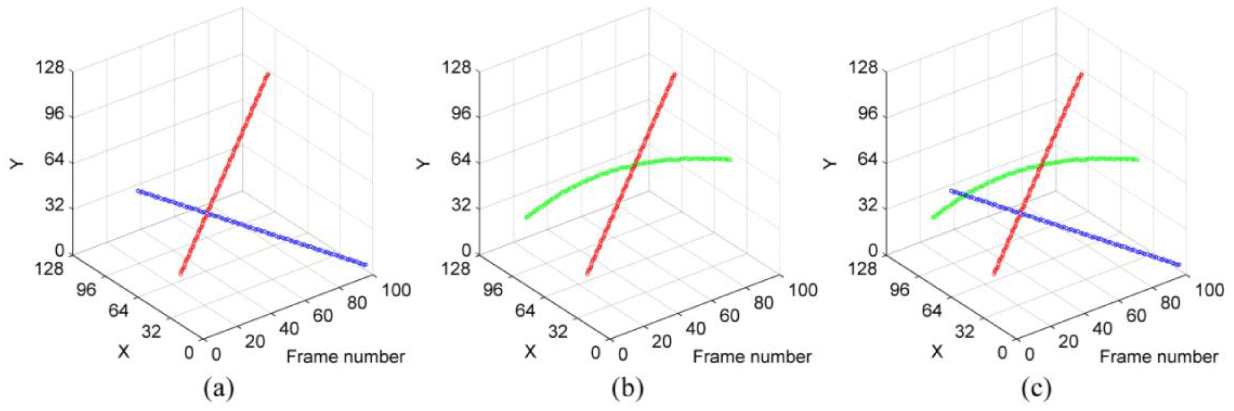
4.2. Multi-Target Detection Test

In the multiple point targets detection test, the size of the simulation images was $128\times 128$ pixels, the sequence length was 100, and the background noise was $n_{\mathit{p}}^{\left(t\right)}~N\left(0,1\right)$. In this test, three types of test cases were used, as shown in Figure 7. In each type of test case, the SNR of point target was in the range of 1.5–3.0, and 1000 simulations were performed for each data group.

After the target trajectories were generated using the DP/DPR point target detection algorithms described in Section 3.3, the multi-target detection performance of each algorithm was evaluated using the detection probability given by Equation (15) and false alarm rate that is given by:

$$P_f=\frac{\mathrm{Number} \mathrm{of} \mathrm{non}-\mathrm{target} \mathrm{ponts} \mathrm{in} \mathrm{all} \mathrm{trajectories}}{\mathrm{Number} \mathrm{of} \mathrm{pixels} \mathrm{in} \mathrm{image} \mathrm{sequence}}.$$

(16)

First, a few common features of the proposed multi-target detection algorithm were analyzed. Because only one coordinate point was extracted from each frame image in each round, and only one trajectory was retained in each round, the correlation complexity of the generated trajectory was significantly reduced; the algorithm complexity was $O\left(N_{\mathrm{tar}}\right)$. As the relative amplitude of the multi-target merit function (Figure 8a) can vary, and when the trajectories of multiple targets intersect, it is difficult to extract a complete target trajectory after one round of the DP/DPR algorithm. However, since median filtering was used to replace the observation data corresponding to the trajectory segment, the trajectory segment could not be extracted repeatedly. In theory, a complete target trajectory can be pieced together after multiple rounds of trajectory detection. In the case of straight line 1, the complete trajectory segment was obtained after three rounds of trajectory detection, as shown in Figure 8b. Target identification errors caused by trajectory intersection could be reduced by trajectory regularization, as shown in Figure 8c.

Next, the performances of six DP/DPR detection algorithms in multi-target detection were tested. The multi-target detection performances of the three DP algorithms in the descending order were as follows: MFF-DP, CSO-DP, and CFO-DP, as shown in Figure 9a–c, and for the three DPR algorithms, the descending order was MFF-DPR, CSO-DPR, and CFO-DPR, as shown in Figure 9d–f. Compared with the DP algorithms, the DPR algorithms had significantly higher multi-target detection performance, as shown in Figure 9g–i.

The detection performance of the multi-target detection algorithms was lower compared to that of the single-target detection algorithms (Figure 6), especially the DP algorithms. The two main reasons for this result were identified through analysis, and they are as follows. First, in the single-target detection algorithms, the only required task after the target points have been obtained is to determine whether the target points are correct. In contrast, in multi-target detection algorithms, it is needed to consider targets with trajectory correlation, but when trajectories are discontinuous, only some trajectory segments can be identified. Second, the mutual influence between multiple target trajectories can affect the detection result.

With the increase in SNR, the false alarm probabilities of the six multi-target detection algorithms exhibited a downward trend, as shown in Figure 10. Moreover, a comparison of results presented in Figure 10a–c reveals that the false alarm probabilities exhibited an upward trend as the number of target trajectories increased. Under SNR > 1.8, the false alarm probabilities of the DPR multi-target detection algorithms were lower than those of DP multi-target detection algorithms. However, when SNR was close to 1.5, the false alarm probabilities of the DPR multi-target detection algorithms could be higher than those of the DP multi-target detection algorithms. This was because the DP multi-target detection algorithms could difficultly extract targets under such a condition, so they could not form trajectories most of the time, which resulted in no incorrect target extraction results.

Finally, the single-frame processing times of different algorithms in single-target detection were compared, as shown in Table 1. In multi-target detection, most time was spent on the DP/DPR merit function updating, as shown in

Table 2. Comparison of the computational efficiencies of the DP/DPR algorithms in multi-target detection.

		CFO-DP/DPR	CSO-DP/DPR	MFF-DP/DPR
Single-frame processing time (ms)	Test case 1	34/65	118/236	161/315
	Test case 2	34/65	119/237	155/313
	Test case 3	53/95	175/353	235/485

. The time required for the target extraction, trajectory correlation, original data updating, and trajectory regularization was about 10% of the merit function updating time. Therefore, developing a method to reduce the algorithm complexity in the merit function updating task effectively will be a future research direction.

5. Conclusions

Aiming to improve the point target detection performance of DP, this paper proposes an MFF-DPR to improve the point target detection probability. First, a second-order DP named the MFF-DP is proposed to reduce noise influence on the pixel state estimation. The current states of pixels on the image plane are estimated by maximizing the addition of the merit functions of the previous two frames and observation data of the current frame. Second, a merit function diffusion suppression structure is proposed. The sequential and reverse observation data are connected head to tail to form a ring structure according to the time reversal symmetry of the DP-TBD. The MFF-DP is constructed to run on the ring structure, and the sequential and reverse merit functions of the MFF-DPs are averaged to obtain the merit function of the MFF-DPR. Finally, the target trajectory is obtained by correlating the extreme points of the merit functions of the MFF-DPR. The simulation and analysis results show that the point target detection algorithm based on the MFF-DPR can achieve a significantly higher performance in point target detection compared with the traditional DP-TBD algorithms. The results also indicate that by merely adding a ring structure, the detection probability of the traditional DP-TBD algorithms can be improved by up to 40% when detecting point targets under the SNR of 1.8.

The MFF-DPR has the same drawback as the traditional second-order DP-TBD. Due to the large search space, calculating the merit function of the MFF-DPR is time-consuming. Fortunately, the processing of each pixel on the image plane based on the MFF-DPR is almost the same; thus, using parallel computing optimization and implementing the GPU programming, the computational speed can be significantly improved. The MFF-DPR is also a batching processing algorithm, which is not suitable for application scenarios with high requirements for real-time performance. Therefore, to enhance the state-of-the-art performance of the current radars and infrared point target detection systems, an improved version of the MFF-DPR is needed; thus, reducing the complexity of the MFF-DPR based on the GPU programming could be a future research direction.

References

1. Xiangzhi, B.; Zhou, F. Analysis of new top-hat transformation and the application for infrared dim small target detection. Pattern Recognit. 2010, 43, 2145–2156. [Google Scholar]
2. Chen, C.P.; Li, H.; Wei, Y.; Xia, T.; Tang, Y.Y. A local contrast method for small infrared target detection. IEEE Trans. Geosci. Remote Sens. 2013, 52, 574–581. [Google Scholar] [CrossRef]
3. Fu, J.; Zhang, H.; Wei, H.; Gao, X. Small bounding-box filter for small target detection. Opt. Eng. 2021, 60, 033107. [Google Scholar] [CrossRef]
4. Ward, M. Target velocity identification using 3-D matched filter with Nelder-Mead optimization. In Proceedings of the IEEE Aerospace Conference, Big Sky, MT, USA, 5–12 March 2011; pp. 1–7. [Google Scholar]
5. Fu, J.; Wei, H.; Zhang, H.; Gao, X. Three-dimensional pipeline Hough transform for small target detection. Opt. Eng. 2021, 60, 023102. [Google Scholar] [CrossRef]
6. Blostein, S.D.; Richardson, H.S. A sequential detection approach to target tracking. IEEE Trans. Aerosp. Electron. Syst. 2002, 30, 197–212. [Google Scholar] [CrossRef]
7. Vo, B.T.; Vo, B.N. A random finite set conjugate prior and application to multi-target tracking. In Proceedings of the 2011 Seventh International Conference on Intelligent Sensors, Sensor Networks and Information Processing, Adelaide, SA, Australia, 6–9 December 2011; pp. 431–436. [Google Scholar]
8. Barniv, Y. Dynamic programming solution for detecting dim moving targets. IEEE Trans. Aerosp. Electron. Syst. 1985, 21, 144–156. [Google Scholar] [CrossRef]
9. Yong, Q.; Cheng, J.L.; Zheng, B. An effective track-before-detect algorithm for dim target detection. Acta Electron. Sin. 2003, 31, 440–443. [Google Scholar]
10. Jiang, H.; Yi, W.; Kong, L.; Yang, X.; Zhang, X. Tracking targets in G0 clutter via dynamic programming based track-before-detect. In Proceedings of the IEEE Radar Conference, Arlington, VA, USA, 10–15 May 2015; pp. 356–361. [Google Scholar]
11. Arnold, J.; Shaw, S.W.; Pasternack, H. Efficient target tracking using dynamic programming. IEEE Trans. Aerosp. Electron. Syst. 1993, 29, 44–56. [Google Scholar] [CrossRef]
12. Tonissen, S.M.; Evans, R.J. Target tracking using dynamic programming: Algorithm and performance. In Proceedings of the 34th IEEE Conference on Decision and Control, New Orleans, LA, USA, 13–15 December 1995; pp. 2741–2746. [Google Scholar]
13. Tonissen, S.M.; Evans, R.J. Peformance of dynamic programming techniques for track-before-detect. IEEE Trans. Aerosp. Electron. Syst. 1996, 32, 1440–1451. [Google Scholar] [CrossRef]
14. Succary, R.; Succary, R.; Kalmanovitch, H.; Shurnik, Y.; Cohen, Y.; Cohenyashar, E.; Rotman, S.R. Point target detection. Infrared Technol. Appl. 2003, 3, 671–675. [Google Scholar]
15. Johnston, L.A.; Krishnamurthy, V. Performance analysis of a dynamic programming track-before-detect algorithm. IEEE Trans. Aerosp. Electron. Syst. 2002, 38, 228–242. [Google Scholar] [CrossRef]
16. Orlando, D.; Ricci, G.; Bar-Shalom, Y. Track-before-detect algorithms for targets with kinematic constraints. IEEE Trans. Aerosp. Electron. Syst. 2011, 47, 1837–1849. [Google Scholar] [CrossRef]
17. Xing, H.; Suo, J.; Liu, X. A dynamic programming track-before-detect algorithm with adaptive state transition set. In International Conference in Communications, Signal Processing, and Systems; Springer: Singapore, 2020; pp. 638–646. [Google Scholar]
18. Guo, Y.; Zeng, Z.; Zhao, S. An amplitude association dynamic programming TBD algorithm with multistatic radar. In Proceedings of the 35th Chinese Control Conference, Chengdu, China, 27–29 July 2016; pp. 5076–5079. [Google Scholar]
19. Yong, Q.; Licheng, J.; Zheng, B. Study on mechanism of dynamic programming algorithm for dim target detection. J. Electron. Inf. Technol. 2003, 25, 721–727. [Google Scholar]
20. Cai, L.; Cao, C.; Wang, Y.; Yang, G.; Liu, S.; Zheng, L. A secure threshold of dynamic programming techniques for track-before-detect. In Proceedings of the IET International Radar Conference, Xi’an, China, 14–16 April 2013; pp. 1–3. [Google Scholar]
21. Grossi, E.; Lops, M.; Venturino, L. Track-before-detect for multiframe detection with censored observations. IEEE Trans. Aerosp. Electron. Syst. 2014, 50, 2032–2046. [Google Scholar] [CrossRef]
22. Zheng, D.-K.; Wang, S.-Y.; Yang, J.; Du, P.-F. A multi-frame association dynamic programming track-before-detect algorithm based on second order markov target state model. J. Electron. Inf. Technol. 2012, 34, 885–890. [Google Scholar]
23. Wang, S.; Zhang, Y. Improved dynamic programming algorithm for low SNR moving target detection. Syst. Eng. Electron. 2016, 38, 2244–2251. [Google Scholar]
24. Sun, L.; Wang, J. An improved track-before-detect algorithm for radar weak target detection. Radar Sci. Technol. 2007, 5, 292–295. [Google Scholar]
25. Lin, H.U.; Wang, S.Y.; Wan, Y. Improvement on track-before-detect algorithm based on dynamic programming. J. Air Force Radar Acad. 2010, 24, 79–82. [Google Scholar]
26. Nichtern, O.; Rotman, S.R. Parameter adjustment for a dynamic programming track-before-detect-based target detection algorithm. EURASIP J. Adv. Signal Process. 2008, 19, 1–19. [Google Scholar] [CrossRef] [Green Version]
Figure 1. Sketchy diagram of the correlation between the observation data X p ( t ) of the current frame (painted green) and the data of the other frames; the regions participating in the state transition decision process are represented in red. (a) First-order DP; (b) second-order DP with the correlation with the observation data of the previous two frames; (c) second-order DP with backtracking; (d) MFF-DP. A point target moves at a speed not greater than v max = 1   pixel/frame.
Applsci 12 01151 g001
Figure 2. The distributions of different merit functions. (a,d) Distributions of merit functions with sequential accumulation at time t = 50; (b,e) distributions of merit functions with reverse accumulation at time t = 50; (c,f) distributions of averaged merit functions with sequential accumulation and reverse accumulation at time t = 50; (ac) the calculation results of the algorithm proposed in Ref. [15]; (df) the calculation results of the MFF-DP algorithm; the size of simulation image is 128 × 128 pixels, the sequence length is N = 100, the background noise is   n p ( t ) ~ N ( 0 , 1 ) , the point target is SNR = 1.8, the initial position is (30, 20), and motion velocity is (0.6, 0.8) pixel/frame.
Applsci 12 01151 g002
Figure 3. Sketchy diagram of the DPR; S Ω ( + t ) and S Ω ( t ) denote the pixel state estimation results of the sequential and reverse DPs at time t , respectively.
Applsci 12 01151 g003
Figure 4. (a) The two trajectories obtained from the coordinate correlation intersect at time t c ; (b,c) two possible target trajectories; each color represents a target identification.
Applsci 12 01151 g004
Figure 5. (a) Test case 1; parameters of the straight-line trajectory were as follows: initial coordinates were (5, 10) and motion velocity was (1.2, 1.1) pixel/frame; (b) test case 2; parameters of the straight-line trajectory were as follows: initial coordinates were (30, 20) and motion velocity was (0.6, 0.8) pixel/frame; (c) test case 3; parameters of the arc trajectory were as follows: motion speed was 1 pixel/frame, arc center coordinates were (64, 64), and arc diameter was 20 pixels.
Applsci 12 01151 g005
Figure 6. Single-target detection probabilities of different DP/DPR algorithms. (ac) Detection probabilities of the DP algorithms; (df) detection probabilities of the DPR algorithms; (gi) detection probability differences between the DPR and DP algorithms; (a,d,g) test case 1; (b,e,h) test case 2; (c,f,i) test case 3.
Applsci 12 01151 g006
Figure 7. (a) Test case 1; (b) test case 2; (c) test case 3. Straight-line trajectory 1 is marked in red, and its initial coordinates were (24,34) and its motion velocity was (0.8, 0.6) pixel/frame; straight-line trajectory 2 is marked in blue, and it had the initial coordinates of (66, 73) and the motion velocity of (−0.6, −0.7) pixel/frame; the arc trajectory is marked in green, and it had the motion speed of 1 pixel/frame, arc center of (64, 46), and the arc radius of 20 pixels. The two straight-line trajectories intersect at (48, 52), while the straight-line trajectory 1 and arc trajectory intersect at (67, 66).
Applsci 12 01151 g007
Figure 8. Test results for test case 3, in which all the three targets had an SNR level of 1.8. (a) Coordinates extracted by the MFF-DPR algorithm in the first, second, and third rounds are marked in red, blue, and green, respectively; (b) trajectories formed by correlating the coordinate points extracted in each round; (c) target trajectories after regularization.
Applsci 12 01151 g008
Figure 9. Multi-target detection probabilities of different DP and DPR algorithms. (ac) Detection probabilities of the DP algorithms; (df) detection probabilities of the DPR algorithms; (gi) differences in detection probabilities between the DPR and DP algorithms; (a,d,g) test case 1; (b,e,h) test case 2; (c,f,i) test case 3.
Applsci 12 01151 g009
Figure 10. False alarm rates of different DP and DPR algorithms in multi-target detection. (a) test case 1; (b) test case 2; (c) test case 3.
Applsci 12 01151 g010