Processing RGB Color Sensors for Measuring the Circadian Stimulus of Artificial and Daylight Light Sources

Featured Application

Accurate practical measurements of the circadian effectiveness of daylight and artificial light sources using RGB color sensors for future human-centered lighting control.

Abstract

The three main tasks of modern lighting design are to support the visual performance, satisfy color emotion (color quality), and promote positive non-visual outcomes. In view of large-scale applications, the use of simple and inexpensive RGB color sensors to monitor related visual and non-visual illumination parameters seems to be of great promise for the future development of human-centered lighting control systems. In this context, the present work proposes a new methodology to assess the circadian effectiveness of the prevalent lighting conditions for daylight and artificial light sources in terms of the physiologically relevant circadian stimulus (CS) metric using such color sensors. In the case of daylight, the raw sensor readouts were processed in such a way that the CIE daylight model can be applied as an intermediate step to estimate its spectral composition, from which CS can eventually be calculated straightforwardly. Maximal CS prediction errors of less than 0.0025 were observed when tested on real data. For artificial light sources, on the other hand, the CS approximation method of Truong et al. was applied to estimate its circadian effectiveness from the sensor readouts. In this case, a maximal CS prediction error of 0.028 must be reported, which is considerably larger compared to daylight, but still in an acceptable range for typical indoor lighting applications. The use of RGB color sensors is thus shown to be suitable for estimating the circadian effectiveness of both types of illumination with sufficient accuracy for practical applications.

1. Introduction

Solid-state lighting considerably increased the possibilities and allowed for a re-interpretation of modern lighting design. The development and use of light-emitting diodes (LEDs), in contrast to conventional light sources, has yielded significant advantages in terms of lifetime, energy savings, environmental benefits, controllability, and spectral tunability [1,2]. Over the past few years, scientific and technological progress in the design of LEDs, including significant improvements in the selection of suitable semiconductor material combinations, the topology of the lattice grid and quantum well structures, the chip packaging, and the coating materials [3,4,5,6,7,8], has led to high luminous efficacies of 150 lm W⁻¹ and beyond, depending on the desired level of color quality [9,10,11]. Typically, an increase in color rendering capabilities, e.g., expressed in terms of the CIE color rendering index (CRI) $R_{\mathrm{a}}$ [12,13,14] or the ANSI/IES TM-30-20 $R_{\mathrm{f}}$ metric [15], occurs at the expense of luminous efficacy so that an adequate trade-off between color quality considerations and energy savings has to be found [16]. Thus, numerous studies have been conducted pursuing the goal of optimizing the spectral compositions of multi-channel LED light sources for achieving an optimal color rendering while still maintaining a sufficiently high level of luminous efficacy [17,18,19,20,21,22,23,24,25,26,27,28,29,30]. At the same time, such multi-channel LED solutions allow for a dynamic adjustment of the lighting conditions to satisfy the users’ visual, emotional, and biological needs in support of positive human outcomes [31,32,33,34,35,36].

Despite these recent technological and conceptual advances in LED and LED-based lighting design, properly dealing with mixed lighting conditions in environments where daylight entry through windows supplements the artificial lighting conditions still poses a defying challenge. Optimizing the latter in some sort of closed-feedback loop under the impact of a second, dynamically changing (daylight) light source defines a difficult regulation problem that so far has only been considered rudimentarily in the literature. A crucial aspect in this context is the proper monitoring of the indoor and outdoor lighting conditions with regard to the lighting parameters most relevant for an appropriate system control to always satisfy certain pre-defined visual and non-visual requirements. In experimental test settings, these kinds of data can be generated straightforwardly by using expensive spectroradiometers or other sophisticated measurement devices. However, in view of large-scale applications, where such “laboratory” devices are not an option due to budgetary constraints, the use of simple and inexpensive RGB color sensors to be applied for this purpose appears to be quite promising [37,38,39,40,41], yet requires a suitable processing of the sensor readouts in order to obtain meaningful measures that can eventually be used as the input for an adequate lighting control [42].

In this context, the present work focuses on the circadian aspects of lighting by proposing a novel sensor-based methodology to assess the circadian effectiveness of the prevalent lighting conditions caused by artificial and daylight light sources using RGB color sensors. As discussed by Babilon et al. [43], circadian effectiveness in lighting can be measured by the physiologically relevant circadian stimulus (CS) metric introduced by Rea and Figueiro [44]. In order to facilitate its application for the lighting practitioner, Truong et al. [45,46] recently published a family of computational approximation methods that can be used to calculate a lighting condition’s CS based on a few easy-to-perform measurements using standard equipment. As will be shown in this work, the sensor readouts of an RGB color sensor, after some suitable processing, can likewise be used as the input for Truong et al.’s approximation method to determine the CS of artificial light sources. For daylight conditions, on the other hand, the RGB output in combination with the CIE daylight model [47] can be used to estimate the corresponding spectral power distributions (SPDs), from which the CS values can be calculated without further approximations by directly applying Rea et al.’s original model.

2. Materials and Methods

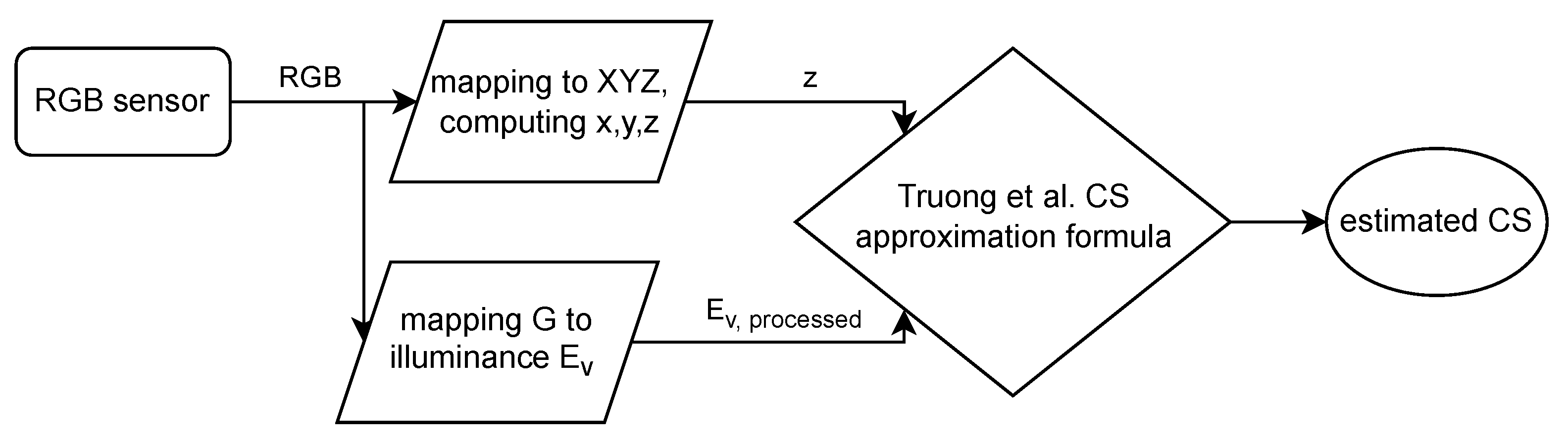
2.1. Circadian Stimulus and Its Approximation

The hormone melatonin has proven to be an excellent and widely used biomarker for assessing how light affects the human circadian system [48,49,50,51,52,53,54,55,56,57,58,59,60,61,62,63,64,65,66,67,68,69,70,71,72,73,74,75,76,77,78,79,80,81,82]. In two independent studies, Brainard et al. [58] and Thapan et al. [59], for example, consistently found that the action spectrum for light-induced nocturnal melatonin suppression peaks at 460 $\mathrm{n}$$\mathrm{m}$ with an approximately 110 $\mathrm{n}$$\mathrm{m}$ broad absorption band at half-maximum sensitivity. Even though the results of both studies were in good agreement over much of the probed wavelength regime, an obvious discontinuity was found in the datasets at about 505 $\mathrm{n}$$\mathrm{m}$, i.e., at a wavelength that would appear as a unique green stimulus causing the spectrally opponent retinal blue versus yellow (b–y) color mechanism to signal zero. As argued by Rea et al. [44,83,84], no single retinal photoreceptor model is capable of adequately describing these observations on the spectral dependencies of melatonin suppression. Instead, all known photoreceptors, including rods, cones, and intrinsically photosensitive retinal ganglion cells (ipRGCs), must be taken into account by explicitly considering their neuroanatomical, neurophysiological, and operational characteristics in order to properly model the experimental findings of human circadian phototransduction [85,86]. Under these prerequisites, Rea et al. [44], by pooling the available nocturnal melatonin suppression data, were able to develop the most complete model of the spectral sensitivity of the human circadian system that, in contrast to single-photopigment-based approaches (e.g., the calculation of $\alpha$-opic quantities [87,88,89], equivalent melanopic lux [90,91], etc.), is capable of adequately describing spectral opponency effects [62,63,73]. Based on their model formalism, Rea et al. introduced a new measure called circadian light ${\mathrm{CL}}_{\mathrm{A}}$, which basically gives the model-weighted irradiance. In order to quantify the circadian effectiveness of arbitrary lighting conditions, they further defined the CS metric, which represents the functional relationship between the ${\mathrm{CL}}_{\mathrm{A}}$ measure and its theoretically provoked melatonin suppression in percent. The CS metric has already been applied successfully in various laboratory and field studies to predict non-visual effects in lighting [92,93,94,95,96,97,98,99,100,101,102,103,104], confirming its physiological relevance.

In order to facilitate the CS calculation for the lighting practitioner, Truong et al. [45,46] recently published a family of computational approximation methods. While the first method models CS as a function of illuminance $E_{\mathrm{v}}$ and the chromaticity coordinate z of the 2 ${}^{\circ }$ standard observer, both measured vertically at eye level, the second method substitutes the latter by using the correlated color temperature (CCT) instead. Although performing CCT measurements is common practice in standard lighting design, which was the main reason for proposing the second approximation method, Truong et al. [46] stated that the CS estimation based on this quantity becomes significantly inaccurate for lighting conditions with CCTs ranging from 3220 $\mathrm{K}$ to 3710 $\mathrm{K}$ and, therefore, is not recommended to be applied in this range. In contrast, an excellent agreement with Rea et al.’s original CS model could be confirmed for the complete range of relevant CCTs when applying the first approximation method. The maximum prediction error ${|\Delta \mathrm{CS}|}_{\max }$ calculated on a comprehensive database of measured SPDs representing both artificial and daylight light sources was found to be less than 0.058 [45]. Therefore, the latter should be used in this work, in particular, since under the assumption that the Luther–Yves condition [42,105,106,107,108] is met sufficiently, a direct mapping from the color sensor’s $RGB$ output to the corresponding CIE $XYZ$ tristimulus values and, thus, to the required z coordinate given by $z=Z/(X+Y+Z)$ can be established. The corresponding model expression is given by:

$$\mathrm{CS}(z,E_{\mathrm{v}})=\left\{\begin{array}{cc}0.7-\frac{0.7}{1+0.016781·{\left(z·E_{\mathrm{v}}^{0.509265}\right)}^{2.268904}}\hfill & \mathrm{if}z>0.195\hfill \\ 0.7-\frac{0.7}{1+0.011376·{\left(z·E_{\mathrm{v}}\right)}^{1.109998}}\hfill & \mathrm{if}z\le 0.195\hfill \end{array}\right.,$$

(1)

and has been validated for white light sources in the range from 10 $\mathrm{lx}$ up to 10,000 $\mathrm{lx}$. It should be noted that the discontinuity at $z=0.195$ represents the spectral opponency effect of the b–y mechanism as discussed above. Equation (1) has been applied successfully for the estimation of CS values in a couple of recently published field studies conducted by Babilon et al. that were intended to provide reliable field measurements of the circadian effectiveness of the prevalent lighting conditions in an office [43] and nursing home environment [109].

2.2. Processing of RGB Color Sensors

This section summarizes the necessary processing steps that are required to be applied to simple RGB color sensors to be used for CS measurements. They include (i) the measurement and determination of the sensors’ spectral sensitivity curves and (ii) the optimization and application of a suitable color correction matrix in order to properly map the sensors’ measured $RGB$ output to standardized CIE $XYZ$ coordinates. In addition, a short introduction to the physical structure and working principle of RGB color sensors is given.

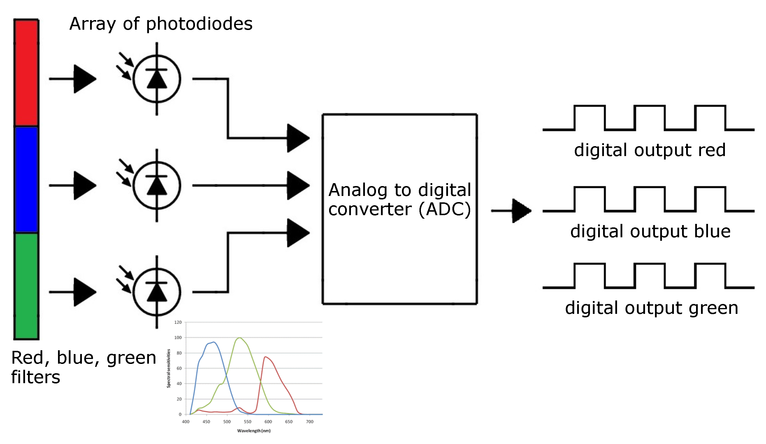
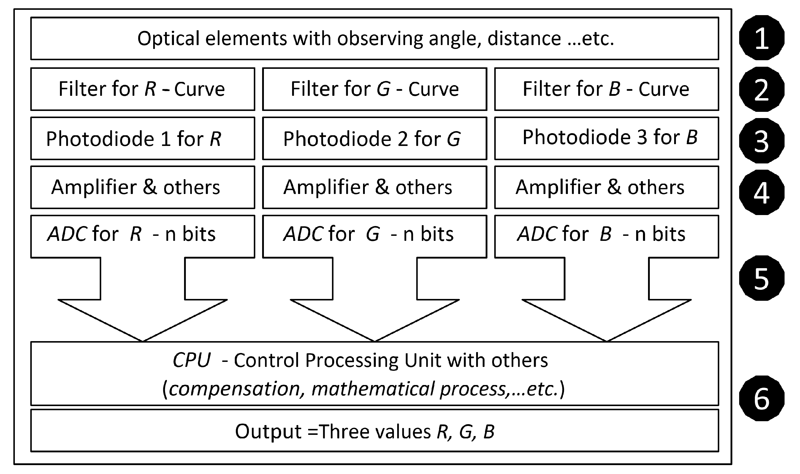
2.2.1. Physical Structure and Working Principle of RGB Color Sensors

An RGB color sensor basically comprises three main components including the underlying semiconductor structure of the photodiodes, the array of optical filters defining its spectral sensitivity, and the electronic circuit used for signal readout [110]. Its physical principle is illustrated in Figure 1. As incident light hits the surface of the RGB color sensor, it is filtered by the red, green, and blue optical bandpass filters attached to the photodiode layer, which combines at least three single photodiodes, i.e., one for each color channel. Without the bandpass filters, a typical silicon photodiode would be sensitive to wavelengths from the ultra-violet up to the infrared region with an absorption maximum located in the range from 800 $\mathrm{n}$$\mathrm{m}$ to 950 $\mathrm{n}$$\mathrm{m}$. The different transmissive color filters are therefore intended to reshape and optimize the spectral response of the color sensor to mimic the trichromatic vision capabilities of the human eye. The correspondingly transmitted photons are thus converted into respective photocurrents, whose amplitudes depend on the spectral composition and irradiance of the incident light. These typically low currents can subsequently be converted into amplified proportional voltage signals using dedicated electronic circuits, such as transimpedance amplifiers or other suitable types of current-to-voltage converters. An analog-to-digital converter (ADC) is eventually applied to convert the amplified voltage outputs into digital signals and, thus, prepare them for further digital processing. Alternatively, a light-to-frequency integrated circuit architecture can be used to directly convert the photocurrents into pulse trains or square waves, whose frequencies are proportional to the irradiance of the correspondingly filtered light [111], which facilitates multiplexing and increases immunity against noise on signal transmittance.

For a schematic overview, Figure 2 summarizes the different structural layers of a color sensor. The first layer comprises the optical elements, such as the housing and aperture, optical lenses, or diffusor plates, that are indented to guarantee a proper, conceivably cosine-corrected irradiation of the sensing area or to adjust the color sensor’s angle of view according to the application requirements. The second layer is composed of the optical bandpass filters $R^{*}\left(\lambda \right)$, $G^{*}\left(\lambda \right)$, and $B^{*}\left(\lambda \right)$ that determine the sensor’s spectral sensitivities $R\left(\lambda \right)$, $G\left(\lambda \right)$, and $B\left(\lambda \right)$. The third layer represents the array of underlying photodiodes, i.e., the actual semiconductor layer, which is responsible for converting the filtered light into corresponding electrical currents. The fourth layer summarizes the electronic circuitry required to convert these photocurrents into proportional, usable signals. The fifth or ADC layer is optional depending on whether a standard current-to-voltage or an integrated circuit architecture is used. In the case of the former, the ADC layer is required to convert the amplified voltage outputs into digital signals. The sixth layer comprises the digital and computational processing of the digital raw sensor signals including the implementation of potential compensation and correction strategies (e.g., to correct for changes in temperature and humidity [112]), which eventually gives the final $RGB$ readouts.

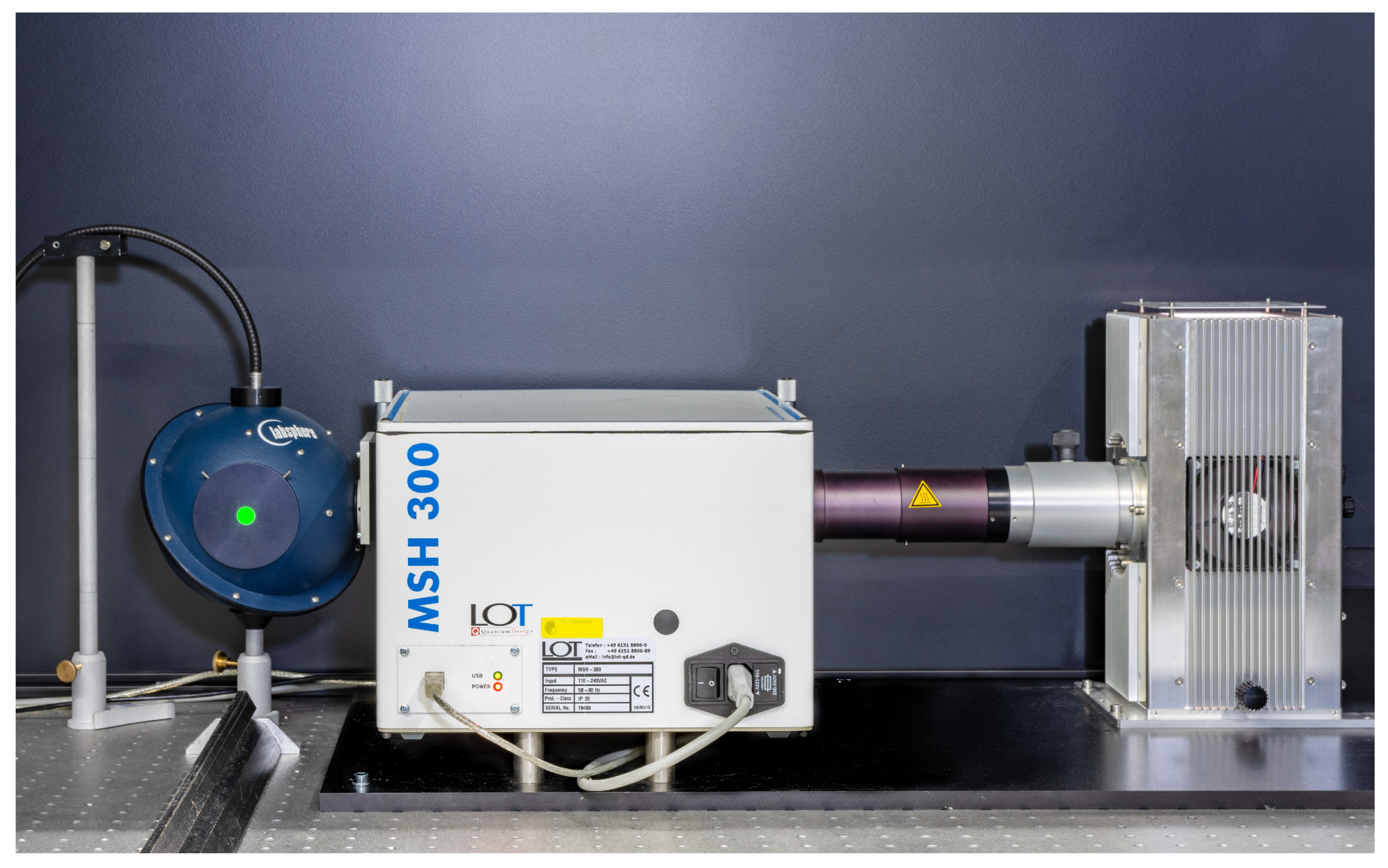
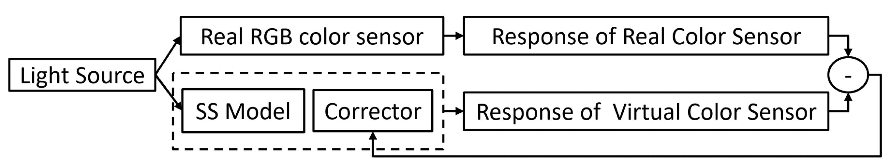
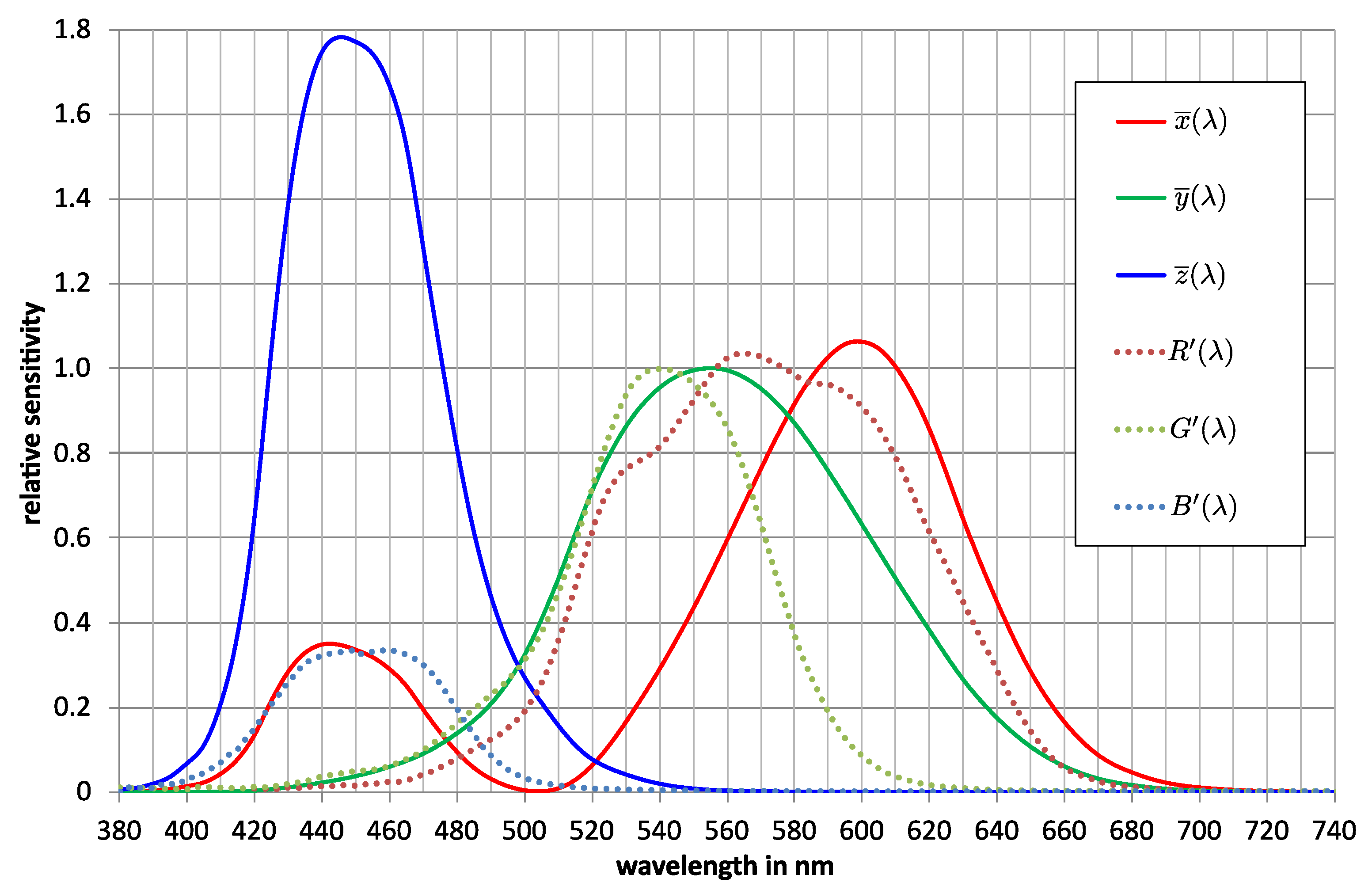
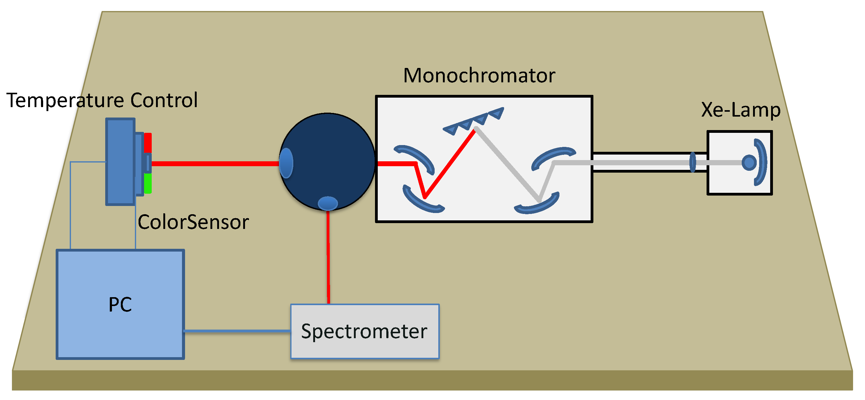
2.2.2. Determination of the Spectral Sensitivity Curves of an RGB Color Sensor

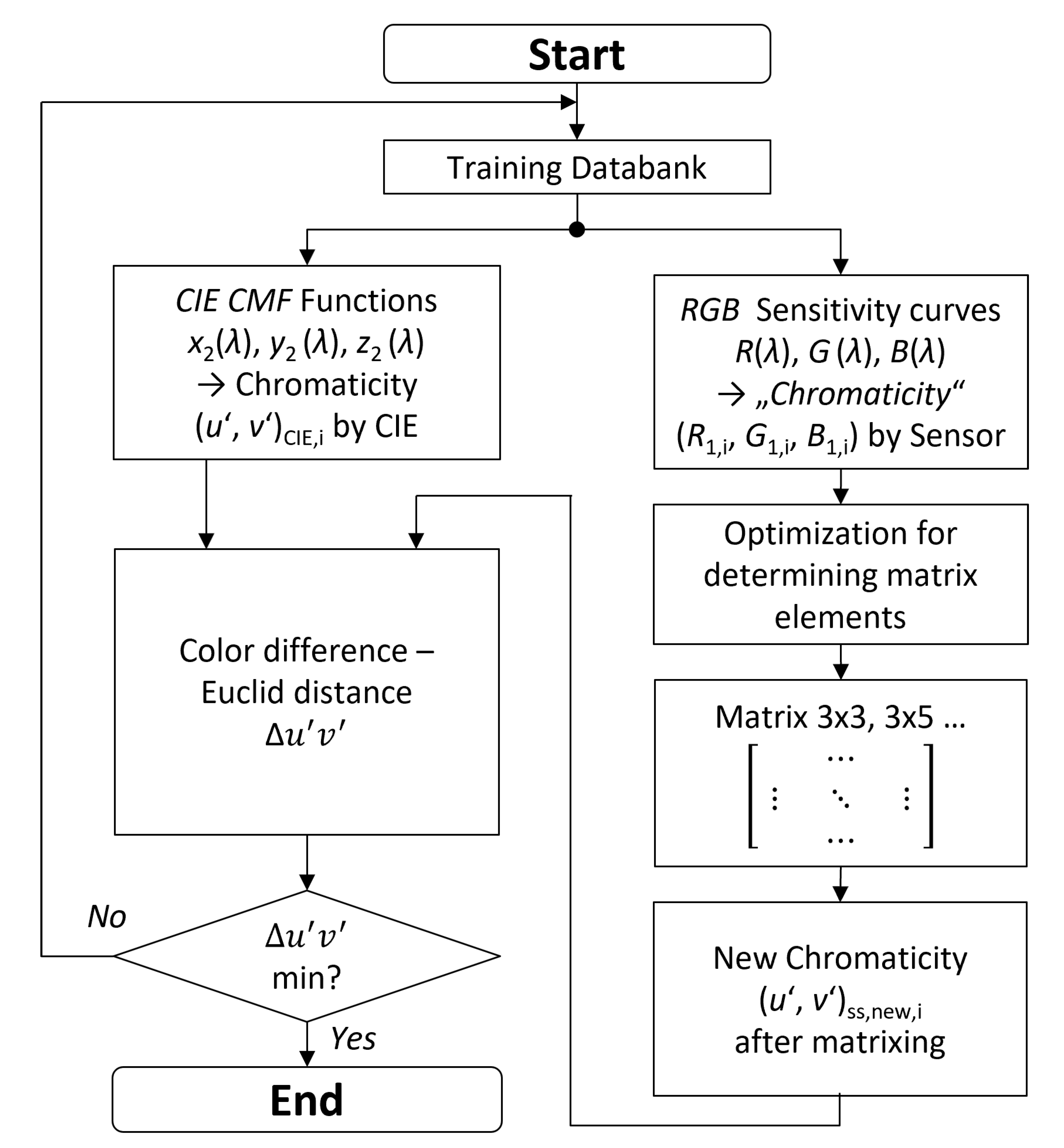
An accurate and precise measurement of the RGB color sensor’s spectral sensitivity functions $R\left(\lambda \right)$, $G\left(\lambda \right)$, and $B\left(\lambda \right)$ is necessary to guarantee an adequate sensor processing for the proper monitoring of the relevant lighting control parameters in mixed lighting conditions as sketched in the Introduction. The literature usually suggests to use a monochromator for this purpose [113,114,115,116,117,118]. An exemplary illustration of the experimental setup is given in Figure 3. As can be seen, a bright white light source of broad spectral composition, e.g., a xenon arc lamp or a Planckian emitter, provides the input to the monochromator. Within the monochromator, the light passing its entrance slit is projected onto an optical diffraction grating. Depending on its pre-selected rotation position, only light of a certain peak wavelength $\lambda$ is thus projected onto the monochromator’s exit slit. The resulting narrowband light output is eventually collected by an integrating sphere for spatial and angular homogenization of its corresponding light distribution [119]. At the same time, it holds both the (temperature-stabilized) color sensor that needs to be characterized and the spectroradiometer used to determine the spectral irradiance of the color stimulus registered by the color sensor.

Based on this setup, the spectral sensitivity $s_k\left(\lambda \right)$ of the kth sensor channel can be determined from the sensor responses $c_k\left(\varphi \left(\lambda \right)\right)$ obtained for a set of selected color stimuli $\varphi \left(\lambda \right)$ provided by the monochromator. According to Myland et al. [42], $s_k\left(\lambda \right)$ can be approximated as follows:

$$s_k\left(\lambda \right)\approx \frac{c_k\left(\varphi \left(\lambda \right)\right)-{\overline{n}}_k}{\delta ·\sum \varphi \left(\lambda \right)\Delta \lambda },$$

(2)

where ${\overline{n}}_k$ is the mean value of random noise observed for a no-light condition, i.e., when the monochromator output is closed and $\delta$ is a constant factor representing the sensor’s gain and integration time settings.

In the present work, an RGB color sensor prototype, which had been developed as part of the INNOSYS project [120] funded by the German Federal Ministry of Education and Research, served as the corresponding test device. Its spectral sensitivities were measured as described above using Equation (2) with a step size of $\Delta \lambda =1 \mathrm{n}\mathrm{m}$, where each of the color stimuli used for probing exhibited a full-width at half-maximum (FWHM) of approximately 2 $\mathrm{n}$$\mathrm{m}$. The corresponding laboratory setting is shown in Figure 4. The measurements were performed using a six-inch integrating sphere (Labsphere Inc., North Sutton, NH, USA) with a highly reflective white PTFE coating, a 300 $\mathrm{W}$ xenon arc lamp connected to an MSH 300 monochromator (Quantum Design GmbH, Darmstadt, Germany), and a Spectro 320D R5 spectroradiometer (Instrument Systems GmbH, Munich, Germany), which was directly attached to the north-pole port of the integrating sphere via a fiber-optic light guide. The main exit port of the integrating sphere at 90°/0° concomitantly served as the sensor mount to ensure a homogeneous light distribution in the color sensor’s field of view.

Due to random errors and systematic uncertainties in the measurement process of the spectral sensitivities, e.g., caused by measurement noise and the finite spectral bandwidth of the color stimuli, discrepancies between model-calculated virtual sensor responses and real sensor measurements must be expected. Thus, in order to improve system performance, the color sensor’s measured sensitivity curves, which give a flawed spectral sensitivity (SS) model, should be corrected accordingly by introducing suitable wavelength-specific correction factors to minimize for each sensor channel the differences in output between the virtual and the real color sensor for a set of representative test light sources, whose SPDs are either known or determined spectroradiometrically. In the present case, a four-channel luminaire prototype [120] consisting of two narrowband monochromatic (red and blue) and two broadband phosphor-converted (cyan and mint-green) LEDs was used to generate 108 different white light test spectra with $R_{\mathrm{a}}>85$ and CCTs in the range from 2700 $\mathrm{K}$ to 6500 $\mathrm{K}$. The corresponding optimization pipeline is illustrated in Figure 5, where the differences between virtual and real channel responses calculated for the different test light spectra serve as feedback for running an interior-point optimization algorithm [121,122,123] to iteratively converge on an optimal set of corrected spectral sensitivities $R^{\prime }\left(\lambda \right)$, $G^{\prime }\left(\lambda \right)$, and $B^{\prime }\left(\lambda \right)$ that yield the same channel outputs as the real color sensor.

For the RGB color sensor used in this work, the corresponding results are summarized in Figure 6 together with the CIE $\overline{x}\left(\lambda \right)$, $\overline{y}\left(\lambda \right)$, and $\overline{z}\left(\lambda \right)$ color matching functions (CMFs) representing the chromatic response sensitivities of the standardized CIE 2° observer [124]. As can be seen, the color sensor’s sensitivity curves considerably deviate from the CMFs of the standard observer. Thus, in order to be able to perform colorimetric measurements, the sensor’s $RGB$ outputs in response to an arbitrary color stimulus need to be mapped onto its corresponding $XYZ$ values as calculated from CIE colorimetry. As is shown in the next section, this mapping can be implemented in the form of a matrix transformation.

2.2.3. Colorimetric Mapping of $RGB$ Sensor Readouts

Based on the measured spectral sensitivities of the specific RGB color sensor used in this work, a nonlinear matrix optimization procedure is proposed in order to minimize the mapping error when transforming from the sensor’s $RGB$ to $XYZ$ tristimulus values. Figure 7 summarizes the optimization workflow. Starting from a training database of n different test light sources, CIE $XYZ$ tristimulus values are calculated first by using:

$$\begin{array}{cc}\hfill X_i& ={\int }_{380}^{780}{S}_{\mathrm{rel},i}\left(\lambda \right)·\overline{x}\left(\lambda \right)d\lambda ,\hfill \\ \hfill Y_i& ={\int }_{380}^{780}{S}_{\mathrm{rel},i}\left(\lambda \right)·\overline{y}\left(\lambda \right)d\lambda ,\hfill \\ \hfill Z_i& ={\int }_{380}^{780}{S}_{\mathrm{rel},i}\left(\lambda \right)·\overline{z}\left(\lambda \right)d\lambda ,\hfill \end{array}$$

(3)

where $S_{\mathrm{rel},i}$ denotes the relative SPD of the ith test light source. Next, the corresponding CIE 1976 uniform chromaticity scale coordinates $(u_{\mathrm{CIE},i}^{\prime },v_{\mathrm{CIE},i}^{\prime })$ [125] are calculated by applying the following set of equations:

$$\begin{array}{c}\hfill u_{\mathrm{CIE},i}^{\prime }=\frac{4X_i}{X_i+15Y_i+3Z_i},\\ \hfill v_{\mathrm{CIE},i}^{\prime }=\frac{9Y_i}{X_i+15Y_i+3Z_i}.\end{array}$$

(4)

A similar processing can be applied to the virtual channel responses of the color sensor. Thus, the sensor’s readouts $R_i{G}_i{B}_i$ for each test light source i of the training set are given by:

$$\begin{array}{cc}\hfill R_i& ={\int }_{380}^{780}{S}_{\mathrm{rel},i}\left(\lambda \right)·R^{\prime }\left(\lambda \right)d\lambda ,\hfill \\ \hfill G_i& ={\int }_{380}^{780}{S}_{\mathrm{rel},i}\left(\lambda \right)·G^{\prime }\left(\lambda \right)d\lambda ,\hfill \\ \hfill B_i& ={\int }_{380}^{780}{S}_{\mathrm{rel},i}\left(\lambda \right)·B^{\prime }\left(\lambda \right)d\lambda .\hfill \end{array}$$

(5)

These readout values are then converted to estimated $X_{\mathrm{SS},i}{Y}_{\mathrm{SS},i}{Z}_{\mathrm{SS},i}$ tristimulus values by applying a matrix transformation of the form:

$$\left(\begin{array}{c}{X}_{\mathrm{SS},i}\\ Y_{\mathrm{SS},i}\\ Z_{\mathrm{SS},i}\end{array}\right)=\left(\begin{array}{cccc}{m}_{1,1}& m_{1,2}& ...& m_{1,n}\\ m_{2,1}& m_{2,2}& ...& m_{2,n}\\ m_{3,1}& m_{3,2}& ...& m_{3,n}\end{array}\right)·\left(\begin{array}{c}{R}_i\\ G_i\\ B_i\\ ...\end{array}\right).$$

(6)

From these tristimulus values, corresponding model chromaticity coordinates $(u_{\mathrm{SS},i}^{\prime },v_{\mathrm{SS},i}^{\prime })$ can be calculated as follows:

$$\begin{array}{c}\hfill u_{\mathrm{SS},i}^{\prime }=\frac{4X_{\mathrm{SS},i}}{X_{\mathrm{SS},i}+15Y_{\mathrm{SS},i}+3Z_{\mathrm{SS},i}},\\ \hfill v_{\mathrm{SS},i}^{\prime }=\frac{9Y_{\mathrm{SS},i}}{X_{\mathrm{SS},i}+15Y_{\mathrm{SS},i}+3Z_{\mathrm{SS},i}}.\end{array}$$

(7)

The prediction error between model and CIE calculation is then given by

$$\Delta u^{\prime }{v}^{\prime }=\frac{1}{n}\sum _i^n\Delta u^{\prime }{v}_i^{\prime }=\frac{1}{n}\sum _i^n\sqrt{{(u_{\mathrm{CIE},i}^{\prime }-u_{\mathrm{SS},i}^{\prime })}^2+{(v_{\mathrm{CIE},i}^{\prime }-v_{\mathrm{SS},i}^{\prime })}^2},$$

(8)

which is used as the target function to be minimized as part of the optimization depicted in Figure 7. Again, the same interior-point optimization algorithm that was used to determine an optimal set of corrected sensor sensitivities was also applied here in order to find the matrix coefficients of Equation (6) that yield the smallest prediction errors $\Delta u^{\prime }{v}^{\prime }$ on the training database of different test light spectra. Instead of using a simple linear $3\times 3$ matrix, the additional introduction of higher-order nonlinear polynomials in the applied matrix transformation may further reduce the prediction errors. Following the studies of Hong et al. [126] and Cheung et al. [127], various polynomials were tested as detailed in

Table 1. Overview of different (higher-) orders of (nonlinear) polynomials to be tested in the applied matrix transformation of Equation (6) according to Hong et al. [126] and Cheung et al. [127].

No.	Size	Content
1	3 × 3	[R G B]
2	3 × 5	[R G B RGB 1]
3	3 × 7	[R G B RG RB GB 1]
4	3 × 8	[R G B RG RB GB RGB 1]
5	3 × 10	[R G B RG RB GB $R^2$ $G^2$ $B^2$ 1]
6	3 × 11	[R G B RG RB GB $R^2$ $G^2$ $B^2$ RGB 1]
7	3 × 14	[R G B RG RB GB $R^2$ $G^2$ $B^2$ RGB $R^3$ $G^3$ $B^3$ 1]
8	3 × 16	[R G B RG RB GB $R^2$ $G^2$ $B^2$ RGB $R^2$G $G^2$B $B^2$R $R^3$ $G^3$ $B^3$]
9	3 × 17	[R G B RG RB GB $R^2$ $G^2$ $B^2$ RGB $R^2$G $G^2$B $B^2$R $R^3$ $G^3$ $B^3$ 1]
10	3 × 19	[R G B RG RB GB $R^2$ $G^2$ $B^2$ RGB $R^2$G $G^2$B $B^2$R R2B G2R B2G $R^3$ $G^3$ $B^3$]
11	3 × 20	[R G B RG RB GB $R^2$ $G^2$ $B^2$ RGB $R^2$G $G^2$B $B^2$R R2B G2R B2G $R^3$ $G^3$ $B^3$ 1]
12	3 × 22	[R G B RG RB GB $R^2$ $G^2$ $B^2$ RGB $R^2$G $G^2$B $B^2$R $R^2$B $G^2$R $B^2$G $R^3$ $G^3$ $B^3$ $R^2$GB R$G^2$B RG$B^2$]

.

After a suitable matrix transform has been found by means of optimization, a verification of the appropriateness of the transform for new light spectra that were not part of the training set is still pending. Thus, a second set of test light sources that differed from the initial training set was available for the purpose of validation. Basically, Equations (3)–(8) were again used to evaluate the final model prediction error for this new set of test light sources as obtained when applying the optimized matrix transform. A comparison of the performance for different matrix sizes and arrangements of nonlinear polynomials is given in Section 3.1.

Finally, it should be noted that the accuracy and predictive performance of this matrix optimization strategy strongly depends on the suitability of the training database with regard to the color sensor’s intended application. Depending on whether the sensor is used for evaluating artificial or daylight light sources, different representative datasets should be considered for performing the optimization in order to derive case-specific matrices that exhibit superior performance compared to using “averaged” matrices only.

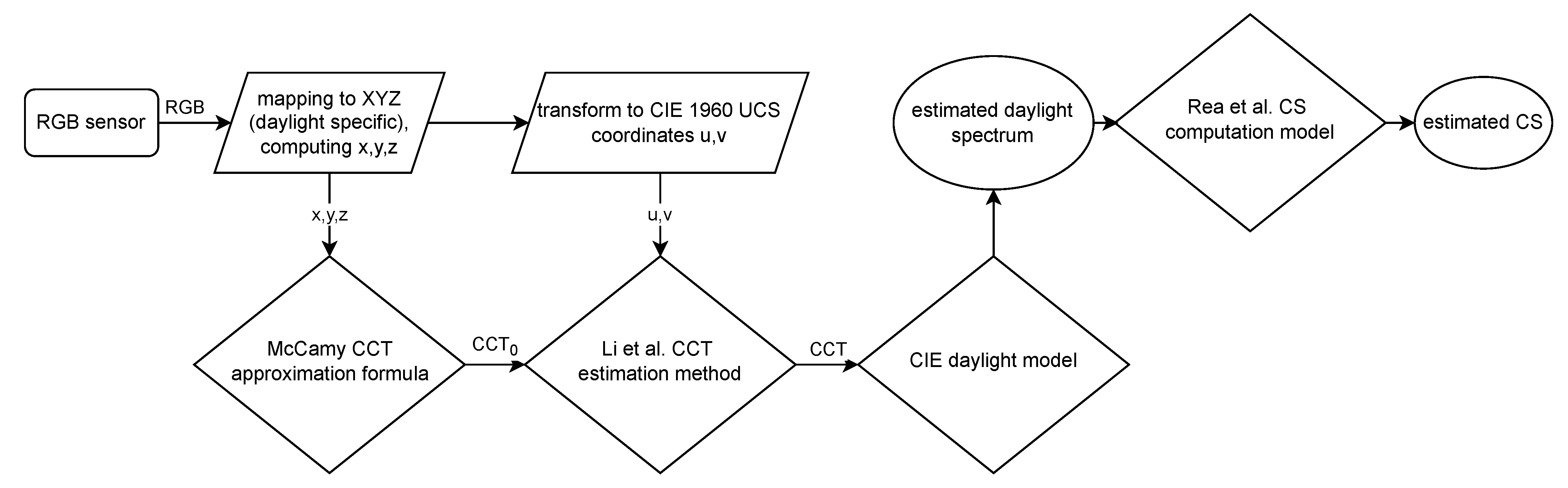
2.3. CIE Daylight Model and CCT Determination for a Daylight Spectral Reconstruction

As shown later in Section 3.1, the combination of the proposed processing for RGB color sensors and the computational model of Truong et al., given by Equation (1) yields a high accuracy in the determination of the CS for artificial light sources. In the case of dealing with daylight light sources, the accuracy can even further be improved by implementing an additional daylight spectral reconstruction step. Once the daylight spectrum is known, its corresponding CS value can be determined directly by applying Rea et al.’s original model as discussed in Section 2.1, which eliminates the need for additional approximations. Thus, the resulting errors in predicting CS for daylight light sources only depends on the applied daylight model (Section 2.3.1) and CCT determination algorithm (Section 2.3.1).

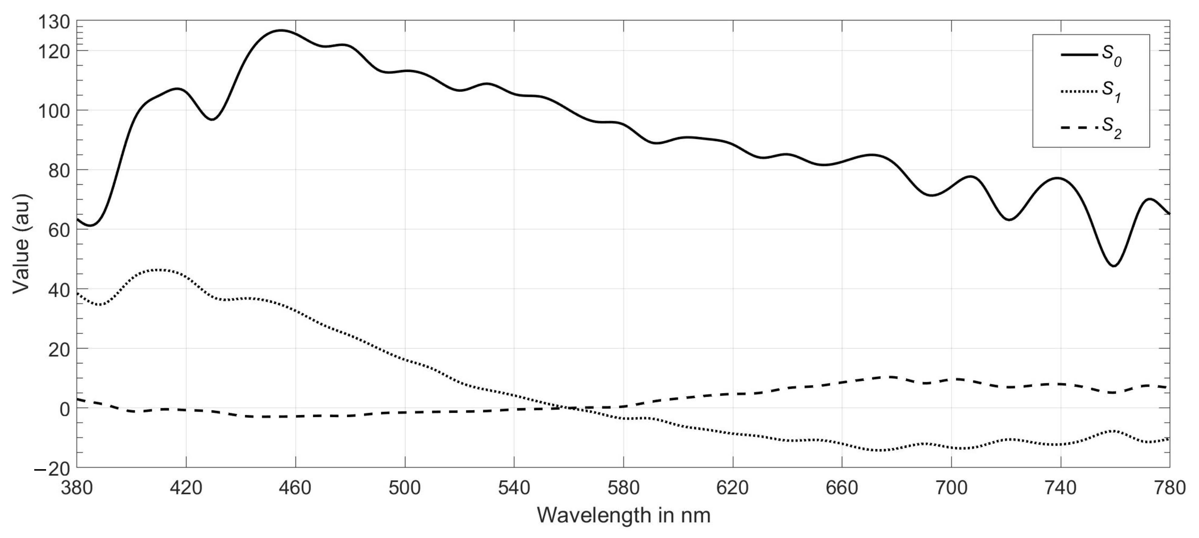
2.3.1. CIE Daylight Model

In this work, the CIE daylight model was applied as a well-accepted method of daylight spectral reconstruction widely used amongst practitioners and scientists. According to CIE [128], its CCT-dependent formalism is given by:

$$S_{\mathrm{daylight}}\left(\lambda \right)=S_0\left(\lambda \right)+S_1\left(\lambda \right)·M_1+S_2\left(\lambda \right)·M_2,$$

(9)

where the auxiliary functions $S_0\left(\lambda \right)$, $S_1\left(\lambda \right)$, and $S_2\left(\lambda \right)$ are illustrated in Figure 8. Their function values are tabulated in the corresponding CIE publication [128]. The chromaticity factors $M_1$ and $M_2$ can be calculated from CCT as follows:

For the CCT range of 5000 $\mathrm{K}$≤ CCT ≤ 7000 $\mathrm{K}$:

$$X_{\mathrm{D}}=\frac{-4.607·{10}^9}{{\mathrm{CCT}}^3}+\frac{2.9678·{10}^6}{{\mathrm{CCT}}^2}+\frac{0.09911·{10}^3}{\mathrm{CCT}}+0.244063,$$

(10)

For the CCT range of CCT > 7000 $\mathrm{K}$

$$X_{\mathrm{D}}=\frac{-2.0064·{10}^9}{{\mathrm{CCT}}^3}+\frac{1.9018·{10}^6}{{\mathrm{CCT}}^2}+\frac{0.24748·{10}^3}{\mathrm{CCT}}+0.244063,$$

(11)

$${\mathit{Y}}_{\mathrm{D}}=-3·X_{\mathrm{D}}^2+2.87·X_{\mathrm{D}}-0.275,$$

(12)

$$M_1=\frac{-1.3515-1.7703·X_{\mathrm{D}}+5.9114·Y_{\mathrm{D}}}{0.0241+0.2562·X_{\mathrm{D}}-0.7341·Y_{\mathrm{D}}},$$

(13)

$$M_2=\frac{0.03-31.4424·X_{\mathrm{D}}+30.0717·Y_{\mathrm{D}}}{0.0241+0.2562·X_{\mathrm{D}}-0.7341·Y_{\mathrm{D}}},$$

(14)

so that the determination of $S_{\mathrm{daylight}}\left(\lambda \right)$ can be traced back to an estimation of the CCT from the color sensor’s $RGB$ readouts. The corresponding algorithmic approach is discussed in the following section.

2.3.2. Determination of the CCT from Sensor Readouts

According to CIE definition [128], the indication of a CCT is only valid for white light sources whose chromaticity coordinates $(u_{\mathrm{r}}^{\prime },2/3v_{\mathrm{r}}^{\prime })$ differ less than:

$$\Delta C=\sqrt{{(u_{\mathrm{r}}^{\prime }-u_{\mathrm{p}}^{\prime })}^2+\frac{4}{9}·{(v_{\mathrm{r}}^{\prime }-v_{\mathrm{p}}^{\prime })}^2}=5·{10}^{-2}$$

(15)

from the chromaticities $(u_{\mathrm{p}}^{\prime },2/3v_{\mathrm{p}}^{\prime })$ of a black body radiator of equivalent temperature. Note that the latter is determined by dropping a perpendicular from the respective light source’s chromaticity coordinates to the Planckian locus as plotted in the CIE 1960 uniform chromaticity scale diagram [129,130].

Thus, the CCT of an arbitrary white light source can be calculated by finding the minimal distance between the light source’s chromaticity coordinates and the Planckian locus by means of solving a nonlinear optimization problem and, therefore, finding the temperature corresponding to the Planckian radiator that causes the most similar color impression. In this work, the method proposed by Li et al. [131] was applied to solve the optimization problem. As it is based on Newton’s method of optimization [132], it by definition only converges locally so that a good initial guess of the optimization’s starting point is necessary to find the absolute minimum. This initial guess of CCT${}_0$ is obtained by applying McCamy’s CCT approximation method to the transformed color sensor readouts $X_{\mathrm{SS}}{Y}_{\mathrm{SS}}{Z}_{\mathrm{SS}}$. The corresponding equations read:

$${\mathrm{CCT}}_0=449·{\eta }^3+3535·{\eta }^2+6823.3·\eta +5520.33,$$

(16)

$$\eta =\frac{x_{\mathrm{SS}}-0.3320}{0.1858-y_{\mathrm{SS}}},$$

(17)

where:

$$\begin{array}{cc}\hfill x_{\mathrm{SS}}& =\frac{X_{\mathrm{SS}}}{X_{\mathrm{SS}}+Y_{\mathrm{SS}}+Z_{\mathrm{SS}}},\hfill \\ \hfill y_{\mathrm{SS}}& =\frac{Y_{\mathrm{SS}}}{X_{\mathrm{SS}}+Y_{\mathrm{SS}}+Z_{\mathrm{SS}}},\hfill \end{array}$$

(18)

give the chromaticity coordinates in the CIE 1931 chromaticity diagram [124]. The transformed sensor readouts are then converted to CIE 1960 uniform chromaticity scale coordinates $(u_{\mathrm{SS}}^{\prime },2/3v_{\mathrm{SS}}^{\prime })$ by applying Equation (7). Using $CC{T}_0$ as the starting point of the optimization, applying the method of Li et al. yields the color temperature of a Planckian radiator whose chromaticities are closest to the chromaticity coordinates of the test light source under consideration. The derived color temperature eventually defines the light source’s CCT.

3. Results

This section summarizes the results of the exemplary measurements that were performed at the Laboratory of Adaptive Lighting Systems and Visual Processing of the Technical University of Darmstadt in order to validate the proposed methodology discussed in the previous sections. Model performance was evaluated in terms of CS differences between the color sensor predictions and Rea et al.’s original model calculations for a selection of both artificial and daylight light sources.

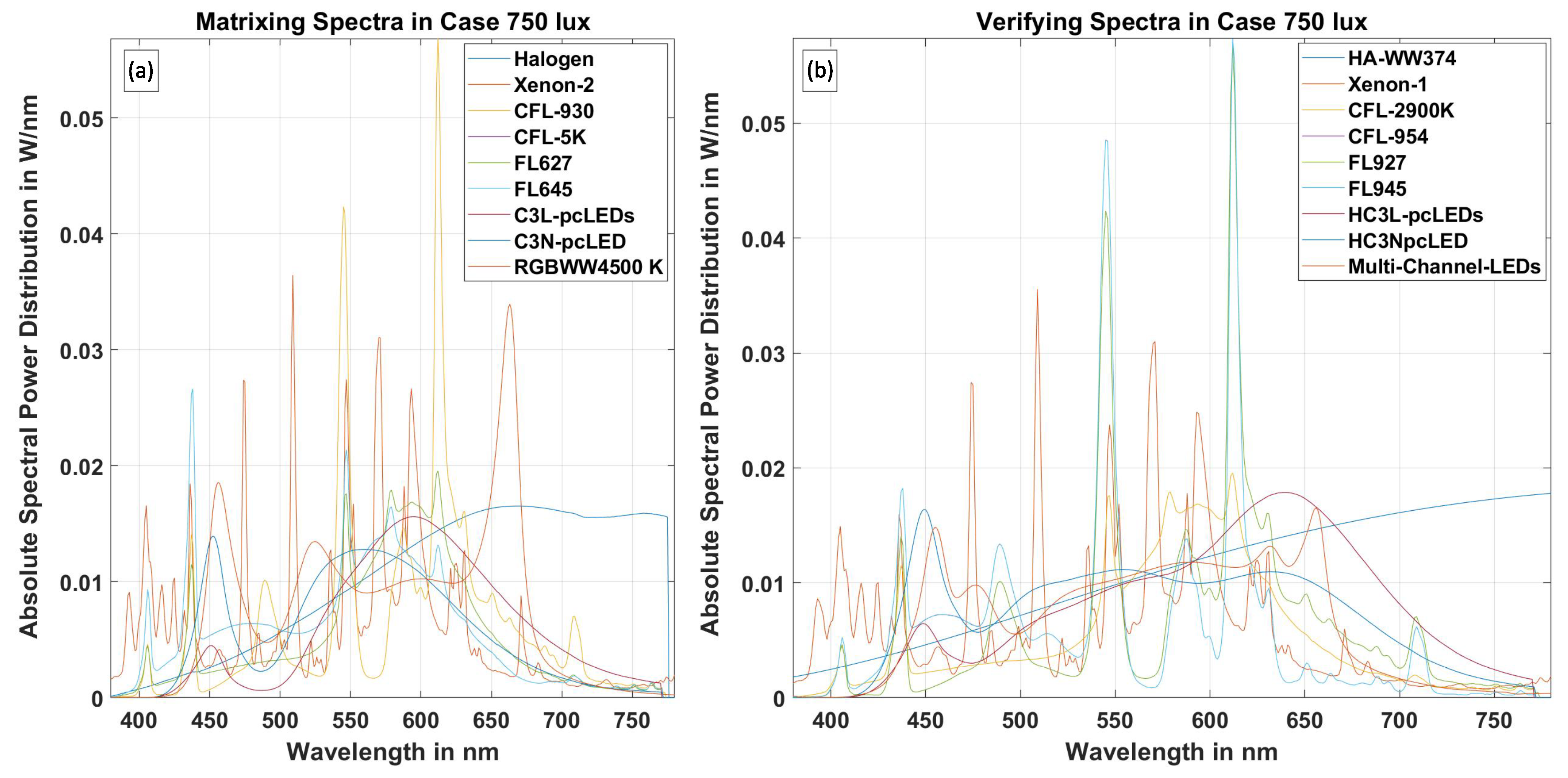
3.1. CS Estimation for Artificial Light Sources

As discussed in Section 2.2.3, $RGB$ sensor responses must be mapped to corresponding $XYZ$ tristimulus values first to calculate the z coordinate required in Truong et al.’s CS approximation formula given by Equation (1). Under the assumption of sensor linearity, an additional linear mapping can be established between the sensor’s green channel output and the likewise-required vertical illuminance $E_{\mathrm{v}}$.

The training database of measured light sources used for constructing these mappings is shown in Figure 9a for a single illuminance level of 750 $\mathrm{lx}$. It comprises different technologies of artificial white light production, including halogen, xenon, compact, and fluorescent lamps, as well as phosphor-converted LEDs (pc-LEDs) and multi-channel LED luminaires. All spectra were measured using a calibrated CSS-45 spectroradiometer (Gigahertz Optik GmbH, Türkenfeld, Germany) with an optical bandwidth of 10 $\mathrm{n}$$\mathrm{m}$ and measurement uncertainties in the x and y coordinates of $\pm 0.002$, in a CCT of ±4% (between 1700 and 17,000 K), and in illuminance E of ±4%. Based on the training data, the virtual sensor responses $R_i{G}_i{B}_i$ were then calculated for different illuminance levels, and the matrix optimization for mapping these sensor responses to $X_{\mathrm{SS},i}{Y}_{\mathrm{SS},i}{Z}_{\mathrm{SS},i}$ tristimulus values was initiated as discussed in Section 2.2.3.

Table 2. Remaining color differences after optimization for different sizes of the corresponding transformation matrix applied to the artificial light sources’ training database.

Name/Par.	Halogen	${\mathbf{Xenon}}_2$	${\mathbf{CFL}}_{930}$	${\mathbf{CFL}}_{5\mathit{K}}$	${\mathbf{FL}}_{627}$	${\mathbf{FL}}_{645}$	${\mathbf{LED}}_{\mathit{C}3\mathit{L}}$	${\mathbf{LED}}_{\mathit{C}3\mathit{N}}$	${\mathbf{RGBW}}_{4\mathit{K}5}$
Δu′v′(3 × 3)$·{10}^3$	3.2	7.4	7.7	1.5	4.5	1.5	4.2	2.7	8.3
Δu′v′(3 × 5)$·{10}^3$	43	4.8	48	12	41	12	51	16	16
Δu′v′(3 × 7)$·{10}^3$	0.00	8.5	5.3	0.00	1.6	0.00	7.0	20	6.4
Δu′v′(3 × 8)$·{10}^3$	4.3	6.9	32	11	40	11	48	7	16
Δu′v′(3 × 10)$·{10}^3$	0.66	2.9	4.5	0.0	0.92	0.0	12	0.00	3.8
Δu′v′(3 × 11)$·{10}^3$	43	7.9	0.00	2.2	37	2.2	42	12	8.1
Δu′v′(3 × 14)$·{10}^3$	7.6	7.1	10	0.00	7.8	0.0	0.0	1.7	6.7
Δu′v′(3 × 16)$·{10}^3$	0.77	8.4	5.7	0.00	3.3	0.00	2.5	1.9	10
Δu′v′(3 × 17)$·{10}^3$	0.77	8.4	5.7	0.00	3.3	0.00	2.5	1.9	10
Δu′v′(3 × 19)$·{10}^3$	5.6	7.2	9.1	0.00	4.3	0.00	0.00	5.7	7.5
Δu′v′(3 × 20)$·{10}^3$	5.6	7.2	9.1	0.00	4.3	0.00	0.00	5.7	7.5
Δu′v′(3 × 22)$·{10}^3$	5.1	6.6	8.9	0.00	2.2	0.00	0.00	3.2	7.2

summarizes the optimization results as calculated on the training data for different sizes of the applied transformation matrix. As can be seen, the overall best performance ($\stackrel{\wedge }{=}$ smallest average prediction error $\Delta u^{\prime }{v}^{\prime }$) was obtained for a simple linear $3\times 3$ transform. Comparably good results can also be observed for matrices of sizes $3\times 19$, $3\times 20$, and $3\times 22$. respectively. However, due to its simplicity, in particular with regard to a potential hardware implementation, the $3\times 3$ approach appears to be most convenient to be applied in the present case. The corresponding optimized matrix elements, as well as the derived relationship between the illuminance $E_{\mathrm{v}}$ and the sensor’s green channel output $G_i$ are depicted in

Table 3. Color sensor’s CS predictions obtained from applying Truong et al.’s approximation method to the transformed color sensor readouts (${\mathrm{CS}}_{2018,\mathrm{Truong}}$) in comparison to the CS predictions of Rea et al.’s original model (${\mathrm{CS}}_{2018,\mathrm{origin}}$) for a selection of artificial light sources from the training dataset at an assumed vertical illuminance of 750 $\mathrm{lx}$. The measurement accuracy for ${\mathrm{CS}}_{2018,\mathrm{origin}}$ is of the order of ±8% due to the measurement uncertainties of the used spectroradiometer. Additionally tabulated are the final $3\times 3$ transformation matrix, as well as the functional relationship between the illuminance and the sensor’s green channel output $G_i$. The annotation “$(Meas.-Calc.)$” in the “Compared parameters” section of the table serves as an indication that the accuracy estimate $|\Delta {\mathrm{CS}}_{2018}|$ for a given light source is determined by the absolute difference between Rea et al.’s and Truong et al.’s corresponding CS predictions as derived from the light source’s radiometric measurements (i.e., “$Meas.$”) and calculated from the resulting sensor readouts (i.e., “$Calc.$”), respectively.

Name/Par.	Halogen	${\mathit{Xenon}}_2$	${\mathit{CFL}}_{3\mathit{K}}$	${\mathit{CFL}}_{5\mathit{K}}$	${\mathit{FL}}_{627}$	${\mathit{FL}}_{645}$	${\mathit{LED}}_{\mathit{C}3\mathit{L}}$	${\mathit{LED}}_{\mathit{C}3\mathit{N}}$	${\mathit{RGBW}}_{4\mathit{K}5}$
${\mathrm{CS}}_{2018}$ and other parameters directly calculated from the measured artificial light spectra
CCT in $\mathrm{K}$	2762	4100	2640	4423	2785	4423	2640	4580	4500
$E_{\mathrm{v}}$ in $\mathrm{lx}$	750	750	750	750	750	750	750	750	750
${\mathrm{CL}}_{\mathrm{A},2018,\mathrm{origin}}$	676.11	471.03	640.73	574.68	529.72	574.73	397.04	430.78	710.02
${\mathrm{CS}}_{2018,\mathrm{origin}}$	0.47	0.40	0.46	0.44	0.43	0.44	0.37	0.39	0.48
${\mathrm{CS}}_{2018}$ and other parameters estimated from the color sensor readouts
$E_{\mathrm{v},\mathrm{processed}}$ in $\mathrm{lx}$	748	794	829	806	806	673	690	669	821
${\mathrm{CS}}_{2018,\mathrm{Truong}}$	0.44	0.40	0.45	0.45	0.45	0.42	0.38	0.40	0.49
Compared parameters
$|\Delta {\mathrm{CS}}_{2018}|$${}_{(Meas.-Calc.)}$	0.0271	0.0072	0.0062	0.0098	0.0234	0.0245	0.0042	0.0105	0.0079
Optimized matrix transformation determined from the artificial light sources training database
$\left[\begin{array}{ccc}5.73\times {10}^5& -4.17\times {10}^5& -2.27\times {10}^5\\ 3.64\times {10}^5& -4.50\times {10}^4& -3.26\times {10}^5\\ -6.61\times {10}^4& 2.04\times {10}^5& 1.13\times {10}^6\end{array}\right]$
Functional relationship for calculating illuminance from sensor output
$E_{\mathrm{v},\mathrm{processed}}=683\times (1.554\times G_i+2.0506)$; $G_i$ from Equation (5)

. In addition, Table 3 tabulates the color sensor’s CS predictions for the light sources from the training dataset at an illuminance of 750 $\mathrm{lx}$ and compares them to the CS values obtained when applying Rea et al.’s original model directly to the measured data instead, which was assumed to represent the ground truth. As can be seen, maximal deviations in CS values of less than 0.028 were observed for this selection of test light sources, which is less than 10% of the CS threshold of 0.3 for which positive effects on sleep quality, mood, and behavior are expected from the literature [43,109]. A sufficiently high measurement accuracy can thus be concluded.

The same holds true when applying the proposed CS estimation to a similar, yet different selection of artificial light sources that were not included in the training dataset used for the determination of the transformation matrix. Their SPDs constituting the validation data are illustrated in Figure 9b. The corresponding model prediction errors $\Delta u^{\prime }{v}^{\prime }$ and $\Delta \mathrm{CS}$ were again calculated and are summarized in

Table 4. Comparison between the color sensor’s CS predictions (${\mathrm{CS}}_{2018,\mathrm{Truong}}$) and Rea et al.’s original model (${\mathrm{CS}}_{2018,\mathrm{origin}}$) for a second set of artificial light sources not included in the training data. Again, the vertical illuminance was assumed to be 750 $\mathrm{lx}$, and the ${\mathrm{CS}}_{2018,\mathrm{origin}}$ measurement accuracy is ±8%. The annotation “$(Meas.-Calc.)$” in the “Compared parameters” section of the table serves as an indication that the accuracy estimate $|\Delta {\mathrm{CS}}_{2018}|$, as well as the colorimetric prediction error $\Delta u^{\prime }{v}^{\prime }$ for a given light source are determined by comparing the corresponding quantities derived from the performed radiometric measurements (i.e., “$Meas.$”) to those calculated from the adequately processed sensor readouts (i.e., “$Calc.$”) as described in this work.

Name/Par.	${\mathit{HA}}_{374}$	${\mathit{Xenon}}_1$	${\mathit{CFL}}_{2\mathit{K}9}$	${\mathit{CFL}}_{954}$	${\mathit{FL}}_{927}$	${\mathit{FL}}_{945}$	${\mathit{LED}}_{\mathit{HC}3\mathit{L}}$	${\mathit{LED}}_{\mathit{HC}3\mathit{N}}$	${\mathit{LED}}_{\mathit{Multi}}$
${\mathrm{CS}}_{2018}$ and other parameters directly calculated from the measured artificial spectra
CCT in $\mathrm{K}$	3300	4058	2785	4390	2640	4390	2797	4870	4000
$E_{\mathrm{v}}$ in $\mathrm{lx}$	750	750	750	750	750	750	750	750	750
${\mathrm{CL}}_{\mathrm{A},2018,\mathrm{origin}}$	897	471	530	620	641	620	727	763	637
${\mathrm{CS}}_{2018,\mathrm{origin}}$	0.51	0.40	0.43	0.45	0.46	0.45	0.48	0.49	0.46
${\mathrm{CS}}_{2018}$ and other parameters estimated from the color sensor readouts
$E_{\mathrm{v},\mathrm{processed}}$ in $\mathrm{lx}$	673	790	766	878	878	748	738	694	815
${\mathrm{CS}}_{2018,\mathrm{Truong}}$	0.49	0.39	0.44	0.47	0.46	0.45	0.46	0.47	0.44
Compared parameters
$|\Delta {\mathrm{CS}}_{2018}|$${}_{(Meas.-Calc.)}$	0.0208	0.0126	0.0143	0.0208	0.0038	0.0083	0.0186	0.0198	0.0203
$\Delta u^{\prime }{v}^{\prime }\times {10}^3$${}_{(Meas.-Calc.)}$	2.42	7.50	4.46	7.04	7.73	7.04	6.46	6.10	4.37

for an illuminance of 750 $\mathrm{lx}$. As can be seen, even smaller errors are observed for the validation than for the original training data, emphasizing that the discussed method including the optimized matrix transform to perform the colorimetric mapping of the sensor responses is most suitable for the determination of sufficiently accurate CS values over a broad variety of lighting technologies usually found in the indoor lighting context.

To ease implementation and to give a better overview of the proposed methodology for the CS estimation of artificial light sources from color sensor responses, Figure 10 depicts the necessary computational steps as a flowchart.

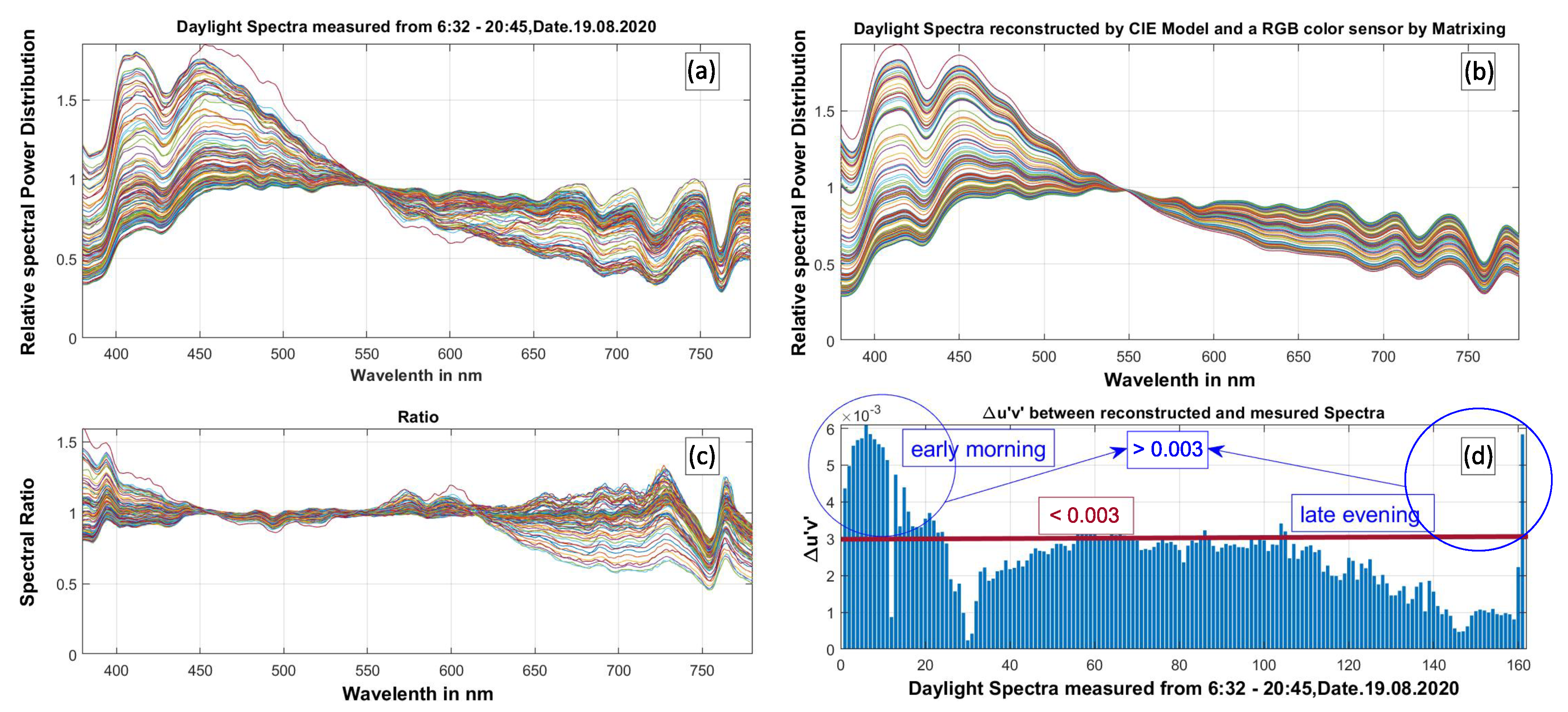
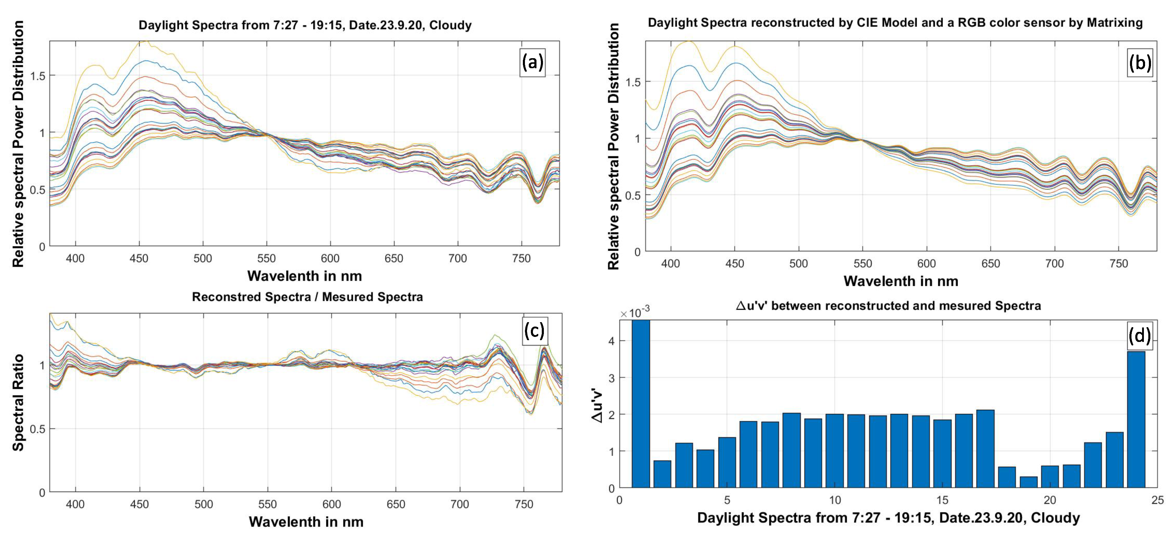
3.2. CS Estimation for Daylight Light Sources

As described in Section 2.3.1 and Section 2.3.2, the CS estimation for daylight spectra can be traced back to the determination of the CCT from the color sensor’s readouts. After converting its $RGB$ output to chromaticity space by applying a daylight-specific transformation matrix, the method of Li et al. can be used to determine the light source’s CCT, which in turn is required to reconstruct its spectral composition by adopting Equations (9)–(14). Once the daylight spectrum is known, the corresponding CS value can directly be calculated without further approximations by making use of Rea et al.’s original model.

In order to derive the daylight-specific transformation matrix and to determine again the relationship between the sensor’s green channel output and $E_{\mathrm{v}}$ for daylight light sources, a dataset of spectral daylight measurements performed on the 19 August 2020 between 6:32 a.m. and 8:45 p.m. in Darmstadt, Hessen, Germany (GPS coordinates 49°51′20.772″ N, 8°39′12.528″ E) using again the CSS-45 spectroradiometer was available for training. The corresponding SPDs are depicted in Figure 11a.

As in the previous section, different matrices were tested for optimal model performance. The corresponding results are shown in

Table 5. Remaining color differences after optimization for different sizes of the daylight-specific transformation matrix applied to the respective training set of measured daylight spectra. Note that only a small, but representative selection of different daylight spectra denoted by their sampling times is shown here.

Sampling Time	06:32	08:03	10:04	12:01	14:02	16:11	18:23	19:04	20:35
Δu′v′(3 × 3)$·{10}^3$	0.5	0.02	0.094	0.053	0.092	0.16	0.15	0.094	1.2
Δu′v′(3 × 5)$·{10}^3$	38	49	6.6	5.4	4.5	3.1	9.5	9.0	33
Δu′v′(3 × 7)$·{10}^3$	1.4	1.5	0.018	0.55	0.2	0.6	0.038	1.1	0.79
Δu′v′(3 × 8)$·{10}^3$	35	48	6.6	5.4	4.5	3.0	9.6	8.7	29
Δu′v′(3 × 10)$·{10}^3$	0.71	0.054	0.13	0.057	0.065	0.17	0.57	0.061	0.78
Δu′v′(3 × 11)$·{10}^3$	31	48	6.5	5.3	4.4	3.0	9.6	8.4	23
Δu′v′(3 × 14)$·{10}^3$	1.1	0.16	0.27	0.11	0.077	0.14	0.068	0.12	2.2
Δu′v′(3 × 16)$·{10}^3$	0.66	0.21	0.3	0.1	0.039	0.21	0.61	0.11	0.8
Δu′v′(3 × 17)$·{10}^3$	0.66	0.21	0.3	0.1	0.039	0.021	0.61	0.11	0.8
Δu′v′(3 × 19)$·{10}^3$	0.23	0.069	0.093	0.039	0.047	0.05	0.094	0.13	0.64
Δu′v′(3 × 20)$·{10}^3$	0.23	0.069	0.93	0.039	0.047	0.05	0.094	0.13	0.64
Δu′v′(3 × 22)$·{10}^3$	0.48	0.019	0.064	0.083	0.051	0.11	0.26	0.17	0.74

for a representative subset of the training data sampled at different measurement times. From these results, it can be confirmed that the use of a simple linear $3\times 3$ matrix again yielded the smallest overall prediction errors. Comparably good results were observed for nonlinear matrices of sizes $3\times 7$, $3\times 10$, and $3\times 14$, respectively. However, following the same argumentation as in Section 3.1, the $3\times 3$ approach, due to its good model performance and simplicity, again appears to be the method of choice for dealing with daylight spectra.

The reconstructed daylight spectra obtained from the color sensor responses by applying the daylight-specific $3\times 3$ chromaticity transformation are thus depicted in Figure 11b. As can be seen from Figure 11c, which illustrates the spectral ratios between the original measurements from the training set and their reconstructed counterparts, the estimated and directly measured daylight spectra were in good agreement in the visually and physiologically most relevant range from about 440 $\mathrm{n}$$\mathrm{m}$ to 630 $\mathrm{n}$$\mathrm{m}$. Larger deviations were only observed in the long- and short-wavelength regime. For $\lambda \le 440\mathrm{n}\mathrm{m}$, the spectral ratio was mostly above unity, while for $\lambda \ge 630\mathrm{n}\mathrm{m}$, the spectral ratio was mostly below unity. As can be seen from Figure 11d, the resulting maximal color difference between measured and reconstructed daylight spectra was $\Delta u^{\prime }{v}_{\max }^{\prime }=0.006$ for lighting conditions captured in the early morning or late evening hours, i.e., when the corresponding CCTs were larger than 10,000 K, causing a bluish rather than a white color perception. However, for daytime measurements at smaller CCTs, the observed color differences were considerably reduced and mostly below the acceptance threshold of $\Delta u^{\prime }{v}_{\mathrm{accept}}^{\prime }=0.003$ as established by Bieske [133], which indicates that the proposed methodology of daylight estimation from $RGB$ sensor responses performed sufficiently accurately in the majority of cases.

From the reconstructed daylight spectra, CS values can now be determined by adopting Rea et al.’s original model definition. At this point, it should be noted that rather than estimating the daylight’s spectral composition from the sensor responses, Truong et al.’s CS approximation method can be used in the same manner as discussed in Section 3.1 for artificial light sources. Hence,

Table 6. Comparison between the color sensor’s CS predictions (${\mathrm{CS}}_{2018,\mathrm{reconstr}.}$) and Rea et al.’s original model (${\mathrm{CS}}_{2018,\mathrm{origin}}$) for a representative selection of daylight spectra from the respective training dataset. The measurement uncertainty for ${\mathrm{CS}}_{2018,\mathrm{origin}}$ is of the order of ±8%. Additionally tabulated are the final $3\times 3$ daylight-specific transformation matrix, as well as the corresponding functional relationship between the illuminance and the sensor’s green channel output $G_i$. Here, the annotation “$(Meas.-Reconstr.)$” indicates that the given accuracy estimates $|\Delta {\mathrm{CS}}_{2018}|$ and colorimetric prediction errors $\Delta u^{\prime }{v}^{\prime }$ are determined by comparing the corresponding quantities derived from the performed radiometric measurements (i.e., “$Meas.$”) and the application of Rea et al.’s model formalism to those obtained by processing the sensor readouts for the subsequent application of the CIE daylight reconstruction method (i.e., “$Reconstr.$”) as proposed in this work. The annotation “$(Meas.-Calc.)$”, on the other hand, again denotes the use of Truong et al.’s approximation method also for daylight spectra.

Sampling Time	06:32	08:03	10:04	12:01	13:02	14:02	16:11	18:23	20:45
${\mathrm{CS}}_{2018}$ and other parameters directly calculated from the measured daylight spectra
CCT in $\mathrm{K}$	10,969	14,170	5557	5614	6324	5679	6240	5389	17,815
$E_{\mathrm{v}}$ in lux	871	5046	57,919	80,580	29,407	87,612	33,370	36,472	203
$x_{\mathrm{meas}.}$	0.2714	0.2610	0.3312	0.3299	0.3162	0.3285	0.3175	0.3351	0.2523
$y_{\mathrm{meas}.}$	0.2903	0.2756	0.3428	0.3402	0.3278	0.3396	0.3304	0.3470	0.2685
${\mathrm{CS}}_{2018,\mathrm{origin}}$	0.613	0.690	0.699	0.699	0.698	0.699	0.698	0.698	0.435
${\mathrm{CS}}_{2018}$ and other parameters estimated from the color sensor readouts by applying the CIE daylight model
${\mathrm{CCT}}_{\mathrm{reconstr}.}$ in $\mathrm{K}$	10,969	14,170	5557	5614	6324	5679	6240	5389	17,815
$E_{\mathrm{v},\mathrm{processed}}$ in $\mathrm{lx}$	879	5015	578,11	80,315	29,447	87,491	33,519	36,431	200
$\Delta u^{\prime }{v}^{\prime }·{10}^3$${}_{(Meas.-Reconstr.)}$	4.4	3.3	2.2	3.1	2.9	2.8	2.1	1.7	5.8
${\mathrm{CS}}_{2018,\mathrm{reconstr}.}$	0.614	0.690	0.699	0.699	0.698	0.699	0.698	0.698	0.433
$|\Delta {\mathrm{CS}}_{2018}|$${}_{(Meas.-Reconstr.)}$	0.001	0.000	0.000	0.000	0.000	0.000	0.000	0.000	0.002
${\mathrm{CS}}_{2018}$ and other parameters estimated from the color sensor readouts by applying Truong et al.’s model
$E_{\mathrm{v},\mathrm{processed}}$ in $\mathrm{lx}$	879	5015	57,811	80,315	29,447	87,491	33,519	36,431	200
$\Delta u^{\prime }{v}^{\prime }·{10}^3$${}_{(Meas.-Calc.)}$	$6.8\times {10}^{-4}$	$4.1\times {10}^{-6}$	$6.8\times {10}^{-5}$	$6.7\times {10}^{-5}$	$4.9\times {10}^{-5}$	$8.1\times {10}^{-5}$	$1.3\times {10}^{-4}$	$1.8\times {10}^{-4}$	$1.0\times {10}^{-3}$
${\mathrm{CS}}_{2018,\mathrm{Truong}}$	0.607	0.688	0.698	0.699	0.697	0.699	0.697	0.697	0.414
$|\Delta {\mathrm{CS}}_{2018}|$${}_{(Meas.-Calc.)}$	0.006	0.002	0.001	0.000	0.001	0.000	0.001	0.001	0.021
Optimized matrix transformation determined from the daylight light sources training database
$\left[\begin{array}{ccc}1.8558& -1.6603& 1.4322\\ 1.1084& -0.23047& 0.53993\\ 0.53135& -0.97596& 6.0956\end{array}\right]$
Functional relationship for calculating illuminance from sensor output
$E_{\mathrm{v},\mathrm{processed}}=683·(1.7175·G_i-19.752)$; $G_i$ from Equation (5)

summarizes for a representative subset of the training data sampled at different measurement times the corresponding results of both approaches and compares them to those obtained for Rea et al.’s original model when being directly applied to the measured daylight spectra without any further sensor processing, which as in the case of artificial light sources, was taken as the ground truth. As can be seen, excellent model performance in terms of predicting CS must be stated for the daylight reconstruction method, where maximal deviations were observed to be of the order of 0.002, which is about ten-times smaller than the maximal CS differences observed for Truong et al.’s approximation method. Thus, even though the latter gives somewhat smaller chromaticity differences $\Delta u^{\prime }{v}^{\prime }$, the combination of RGB sensor output and CIE daylight model yields a significantly better performance in terms of predicting CS values from color sensor readouts with an almost perfect accuracy.

The reason for the somewhat larger chromaticity differences obtained by applying the spectral reconstruction method can be identified in the way $S_{\mathrm{daylight}}\left(\lambda \right)$ is determined. As can be seen from Equations (9)–(14), the calculation of spectra defining the CIE daylight locus is solely based on the CCT parameter and, therefore, neglects chromaticity information. However, as the true chromaticities of the measured daylight spectra may differ from those modeled by the CIE daylight locus (even when the CCT is found to be the same), non-negligible chromaticity errors are likely to occur. Nonetheless, with regard to the main goal of the present work, i.e., the proper estimation of the circadian effectiveness of the prevalent lighting conditions from color sensor responses, the spectral reconstruction approach still appears to be the favored method because of its high accuracy in terms of predicting CS values for daylight light sources.

As for the case of artificial light sources, a validation of the proposed methodology should be performed on a second dataset of measured daylight conditions that were not included in the training data. Corresponding measurements were taken on 23 September 2020 between 7:27 a.m. and 19:15 p.m. at the same measurement location and by using the same measurement device as for the first round of spectral daylight acquisitions. The measured SPDs of the second round are thus visualized in Figure 12a, where the same daylight-specific $3\times 3$ transformation matrix as optimized for the training data was used to convert the resulting color sensor responses to the chromaticity space for the CCT calculation and subsequent spectral modeling. The corresponding CIE model results are depicted in Figure 12b. Compared to the training data, similar findings can be reported on the spectral ratios between the original measurements of daylight spectra used for validation and their reconstructed estimations illustrated in Figure 12c. A good agreement ($\stackrel{\wedge }{=}$ spectral ratio close to unity) can again be confirmed in the wavelength range from 440 $\mathrm{n}$$\mathrm{m}$ to 630 $\mathrm{n}$$\mathrm{m}$, while considerably larger deviations were obtained for shorter or longer wavelengths. As can be seen from Figure 12d, the maximal chromaticity difference $\Delta u^{\prime }{v}_{\max }^{\prime }$ was of the same order as observed for the training set, where again the greatest differences occurred in the early morning and late evening hours. However, in general, the resulting chromaticity differences for the validation data were well below the acceptance threshold defined by Bieske, which again emphasizes the suitability of the proposed approach.

Finally,

Table 7. Comparison between the color sensor’s CS predictions (${\mathrm{CS}}_{2018,\mathrm{reconstr}.}$) and Rea et al.’s original model (${\mathrm{CS}}_{2018,\mathrm{origin}}$) for a second set of measured daylight spectra not included in the training data. The measurement uncertainty for ${\mathrm{CS}}_{2018,\mathrm{origin}}$ is of the order of ±8%. Here, the annotation “$(Meas.-Reconstr.)$” indicates that the given accuracy estimates $|\Delta {\mathrm{CS}}_{2018}|$ and colorimetric prediction errors $\Delta u^{\prime }{v}^{\prime }$ are determined by comparing the corresponding quantities derived from the performed radiometric measurements (i.e., “$Meas.$”) and the application of Rea et al.’s model formalism to those obtained by processing the sensor readouts for the subsequent application of the CIE daylight reconstruction method (i.e., “$Reconstr.$”) as proposed in this work. The annotation “$(Meas.-Calc.)$”, on the other hand, again denotes the use of Truong et al.’s approximation method also for daylight spectra.

Sampling Time	07:27	10:03	11:06	12:03	13:05	14:07	15:10	16:12	19:14
${\mathrm{CS}}_{2018}$ and other parameters directly calculated from the measured daylight spectra
CCT in $\mathrm{K}$	12,464	8033	6313	5651	5914	5853	5470	8174	16,066
$E_{\mathrm{v}}$ in lux	401	9397	23,940	58,212	39,463	43,150	71,006	15,058	4613
$x_{\mathrm{meas}.}$	0.2652	0.2942	0.3163	0.3291	0.3236	0.3248	0.3332	0.2919	0.2568
$y_{\mathrm{meas}.}$	0.2831	0.3066	0.3293	0.3413	0.3364	0.3376	0.3449	0.3081	0.2705
${\mathrm{CS}}_{2018,\mathrm{origin}}$	0.528	0.693	0.697	0.699	0.698	0.699	0.699	0.696	0.561
${\mathrm{CS}}_{2018}$ and other parameters estimated from the color sensor readouts by applying the CIE daylight model
${\mathrm{CCT}}_{\mathrm{reconstr}.}$ in $\mathrm{K}$	12,561	8044	6306	5647	5907	5845	5470	8146	16,309
$E_{\mathrm{v},\mathrm{processed}}$ in $\mathrm{lx}$	402	9389	24,051	58,213	39,593	43,239	70,871	15,180	454
$\Delta u^{\prime }{v}^{\prime }·{10}^3$${}_{(Meas.-Reconstr.)}$	4.6	1.8	2.0	2.0	1.9	1.9	2.0	0.57	3.7
${\mathrm{CS}}_{2018,\mathrm{reconstr}.}$	0.530	0.693	0.697	0.699	0.698	0.699	0.699	0.696	0.559
$|\Delta {\mathrm{CS}}_{2018}|$${}_{(Meas.-Reconstr.)}$	0.002	0.000	0.000	0.000	0.000	0.000	0.000	0.000	0.001
${\mathrm{CS}}_{2018}$ and other parameters estimated from the color sensor readouts by applying Truong et al.’s model
$\Delta u^{\prime }{v}^{\prime }·{10}^3$${}_{(Meas.-Calc.)}$	0.47	0.0	0.174	0.12	0.182	0.196	0.0596	0.403	0.85
${\mathrm{CS}}_{2018,\mathrm{Truong}}$	0.517	0.691	0.696	0.698	0.698	0.698	0.699	0.695	0.548
$|\Delta {\mathrm{CS}}_{2018}|$${}_{(Meas.-Calc.)}$	0.011	0.002	0.001	0.001	0.001	0.001	0.001	0.001	0.013

summarizes the different model predictions when applying the daylight reconstruction approach in comparison to Truong et al.’s approximation method and the direct calculations performed on the set of measured validation data using Rea et al.’s original CS definition. As can be seen, similar results were obtained as reported for the set of training data: despite showing again slightly larger chromaticity deviations, the daylight reconstruction approach still outperformed Truong et al.’s approximation method in terms of CS prediction accuracy, which allowed for a proper estimation of the circadian effectiveness from color sensor responses even for “unknown” daylight conditions that were not included in the initial training database. To support reproducibility, the flowchart of Figure 13 eventually summarizes the proposed daylight reconstruction strategy and gives an overview of the required computational steps for a subsequent CS estimation.

4. Conclusions and Outlook

In this work, a novel sensor-based methodology was proposed to assess the circadian effectiveness of the prevalent lighting conditions caused by artificial and daylight light sources using simple and inexpensive RGB color sensors that can easily be integrated into modern lighting systems for proper monitoring and advanced lighting control. It was shown that the sensor readouts, after some suitable processing, can be used to estimate CS, a measure of circadian effectiveness, with high accuracy. For artificial light sources, the $RGB$ sensor responses were mapped to CIE $XYZ$ tristimulus values first by applying a suitable 3 transformation matrix. From these $XYZ$ values, the corresponding chromaticity coordinate z can be calculated. Together with the lighting condition’s illuminance $E_{\mathrm{v}}$, this provides the input for the application of Truong et al.’s approximation formula, which yields an estimate for the circadian effectiveness in terms of CS. Compared to Rea et al.’s original model description, only small model prediction errors (typically less than 0.028 $\Delta CS$) were observed for a broad variety of artificial test light sources, emphasizing the suitability of the proposed approach with regard to predicting sufficiently accurate CS values from $RGB$ sensor output for light sources usually found in the indoor lighting context.

For daylight light sources, on the other hand, an estimation of their spectral compositions from $RGB$ sensor readouts was performed first by adopting the CIE daylight model. After converting the color sensor’s $RGB$ output to the CIE 1960 chromaticity space by applying a daylight-specific $3\times 3$ matrix transform and subsequent linear transformation, i.e., from $XYZ$ to $(u^{\prime },2/3v^{\prime })$, a nonlinear optimization method was used to determine the daylights’ CCTs, which are the main input in the CIE model to reconstruct their spectral compositions. With known illuminance $E_{\mathrm{v}}$, corresponding CS values could then be calculated without further approximations by applying Rea et al.’s original model to the estimated daylight spectra. Compared to Rea et al.’s model when applied directly to the measured light source data, the proposed daylight reconstruction method yielded excellent model performance with maximal prediction errors $\Delta C{S}_{\max }$ of less than 0.002 for both known (i.e., part of the training data) and unknown (i.e., not part of the training data) daylight conditions. In addition, it could be shown that for both test cases, the daylight reconstruction approach outperformed Truong et al.’s approximation method in terms of CS prediction accuracy, making the former the appropriate method of choice when dealing with daylight conditions.

When comparing the results achieved for both artificial sources and daylight, it becomes clear that there might be still room for improvements regarding the application of the proposed methodology for the estimation of circadian effectiveness for artificial lighting conditions. Whereas for daylight, the reported model prediction errors were more or less of the same small order (see Table 6 and Table 7), considerably larger discrepancies and greater errors were observed for their artificial counterparts (see Table 3 and Table 4). Instead of using Truong et al.’s approximation method, it could therefore be expedient to also implement a spectral reconstruction strategy for artificial light sources so that Rea et al.’s original model can be applied without any further approximations. The first approaches for multi-channel sensors found in the literature using a multilayer perceptron seem to be quite promising for this purpose and report reconstructed SPD errors of less than 2% [134,135]. However, it remains questionable whether such a high accuracy can also be achieved with a simple RGB color sensor. Of course, the methodology proposed in this work could easily be adapted to be used in conjunction with a multi-channel sensor instead, which potentially would increase spectral reconstruction accuracy. However, additional experiments will be required to draw final conclusions.

For daylight conditions, on the other hand, the procedure described in this work so far dealt with outdoor measurements only. Nonetheless, with regard to the establishment of human-centered lighting control strategies, the accuracy of the proposed methodology must still be confirmed for daylight, which is measured indoors behind windows that are made of glass or other materials. As long as these transmissive materials are chiefly aselective in the visible regime [136,137,138] and, thus, only diminish the entering daylights’ absolute levels of illuminance without changing their spectral composition, a similar accuracy as reported for the outdoor measurements can be expected to be observed when applying the proposed method to calculate CS for daylight conditions that are measured indoors. However, in the case that the spectral transmittance of the window material is strongly wavelength dependent, Truong et al.’s approximation method needs to be applied, which, as shown in this work, considerably reduces CS prediction accuracy (at least in its current form; see the previous paragraph). For both cases, though, dedicated experiments are required to confirm these expectations and eventually quantify the respective accuracies.

Regarding the issue of proper system integration and testing, ongoing research by our lab further addresses the lighting control problem in realistic application scenarios. For this purpose, a multi-channel IoT floor lamp prototype has recently been developed with contributions from some of the present authors [139] that allows for the implementation of additional color sensor devices to monitor the ambient lighting conditions as sketched in the Introduction. Thus, in order to account for potential changes in the ambient lighting conditions, color sensor feedback is intended to serve as suitable input for adaptively updating the lighting control parameters to achieve constant or pre-defined indoor lighting conditions that may for example keep the circadian effectiveness always at an optimal level. Corresponding field tests are currently under preparation, for which the current work provides the theoretical and methodological background. At the same time, it will guide others to develop similar sensor-based strategies for an advanced lighting control, which will help to drive the momentum towards the integration of human-centered lighting solutions into our daily lives.

References

1. Schubert, E.F.; Kim, J.K. Solid-state light sources getting smart. Science 2005, 308, 1274–1278. [Google Scholar] [CrossRef] [PubMed]
2. Protzman, J.B.; Houser, K.W. LEDs for general illumination: The state of the science. LEUKOS 2006, 3, 121–142. [Google Scholar] [CrossRef]
3. Zhang, T.; Tang, H.; Li, S.; Wen, Z.; Xiao, X.; Zhang, Y.; Wang, F.; Wang, K.; Wu, D. Highly efficient chip-scale package LED based on surface patterning. IEEE Photonics Technol. Lett. 2017, 29, 1703–1706. [Google Scholar] [CrossRef]
4. Usman, M.; Mushtaq, U.; Zheng, D.; Han, D.; Rafiq, M.; Muhammad, N. Enhanced internal quantum efficiency of bandgap-engineered green w-shaped quantum well light-emitting diode. Appl. Sci. 2019, 9, 77. [Google Scholar] [CrossRef] [Green Version]
5. Hsiang, E.; He, Z.; Huang, Y.; Gou, F.; Lan, Y.; Wu, S. Improving the power efficiency of micro-LED displays with optimized LED chip sizes. Crystals 2020, 10, 494. [Google Scholar] [CrossRef]
6. Wei, Y.; Gao, Z.; Liu, S.; Chen, S.; Xing, G.; Wang, W.; Dang, P.; Al Kheraif, A.A.; Li, G.; Lin, J. Highly efficient green-to-yellowish-orange emitting Eu2+-doped pyrophosphate phosphors with superior thermal quenching resistance for w-LEDs. Adv. Opt. Mater. 2020, 8, 1901859. [Google Scholar] [CrossRef]
7. Lian, L.; Li, Y.; Zhang, D.; Zhang, J. Synthesis of highly luminescent InP/ZnS quantum dots with suppressed thermal quenching. Coatings 2021, 11, 581. [Google Scholar] [CrossRef]
8. Liang, G.; Yu, S.; Tang, Y.; Lu, Z.; Yuan, Y.; Li, Z.; Li, J. Enhancing luminous efficiency of quantum dot-based chip-on-board light-emitting diodes using polystyrene fiber mats. IEEE Trans. Electron Devices 2020, 67, 4530–4533. [Google Scholar] [CrossRef]
9. Sadeghi, S.; Kumar, B.G.; Melikov, R.; Aria, M.M.; Jalali, H.B.; Nizamoglu, S. Quantum dot white LEDs with high luminous efficiency. Optica 2018, 5, 793–802. [Google Scholar] [CrossRef]
10. Taki, T.; Strassburg, M. Review—Visible LEDs: More than efficient light. ECS J. Solid State Sci. Technol. 2019, 9, 015017. [Google Scholar] [CrossRef]
11. Pattison, M.; Hansen, M.; Bardsley, N.; Elliott, C.; Lee, K.; Pattison, L.; Tsao, J. 2019 Lighting R&D Opportunities; Technical Report DOE/EE-2008 8189; U.S. Department of Energy: Washington, DC, USA, 2020. [CrossRef]
12. Commission Internationale de l’Éclairage. Method of Measuring and Specifying Colour Rendering Properties of Light Sources—CIE Technical Report 13.1; CIE: Vienna, Austria, 1965. [Google Scholar]
13. Commission Internationale de l’Éclairage. Method of Measuring and Specifying Colour Rendering Properties of Light Sources—CIE Technical Report 13.2; CIE: Vienna, Austria, 1974. [Google Scholar]
14. Commission Internationale de l’Éclairage. Method of Measuring and sPecifying Colour Rendering Properties of Light Sources—CIE Technical Report 13.3; CIE: Vienna, Austria, 1995. [Google Scholar]
15. American National Standards Institute, Inc. IES Method for Evaluating Light Source Color Rendition; ANSI/IES TM-30-20; American National Standards Institute, Inc.: New York, NY, USA, 2019. [Google Scholar]
16. Zhang, F.; Xu, H.; Wang, Z. Optimizing spectral compositions of multichannel LED light sources by IES color fidelity index and luminous efficacy of radiation. Appl. Opt. 2017, 56, 1962–1971. [Google Scholar] [CrossRef] [PubMed]
17. Žukauskas, A.; Vaicekauskas, R.; Ivanauskas, F.; Gaska, R.; Shur, M.S. Optimization of white polychromatic semiconductor lamps. Appl. Phys. Lett. 2002, 80, 234–236. [Google Scholar] [CrossRef]
18. Žukauskas, A.; Vaicekauskas, R.; Ivanauskas, F.; Shur, M.S.; Gaska, R. Optimization of white all-semiconductor lamp for solid-state lighting applications. Int. J. High Speed Electron. Syst. 2002, 12, 429–437. [Google Scholar] [CrossRef]
19. Ries, H.; Leike, I.; Muschaweck, J.A. Optimized additive mixing of colored light-emitting diode sources. Opt. Eng. 2004, 43, 1531–1536. [Google Scholar] [CrossRef]
20. Lin, K.C. Approach for optimization of the color rendering index of light mixtures. J. Opt. Soc. Am. A 2010, 27, 1510–1520. [Google Scholar] [CrossRef]
21. Smet, K.; Ryckaert, W.R.; Pointer, M.R.; Deconinck, G.; Hanselaer, P. Optimal colour quality of LED clusters based on memory colours. Opt. Express 2011, 19, 6903–6912. [Google Scholar] [CrossRef]
22. Smet, K.A.G.; Ryckaert, W.R.; Pointer, M.R.; Deconinck, G.; Hanselaer, P. Optimization of colour quality of LED lighting with reference to memory colours. Light. Res. Technol. 2012, 44, 7–15. [Google Scholar] [CrossRef]
23. Chalmers, A.N.; Soltic, S. Light source optimization: Spectral design and simulation of four-band white-light sources. Opt. Eng. 2012, 51, 044003. [Google Scholar] [CrossRef]
24. Bulashevich, K.A.; Kulik, A.V.; Karpov, S.Y. Optimal ways of colour mixing for high-quality white-light LED sources. Phys. Status Solidi A 2015, 212, 914–919. [Google Scholar] [CrossRef]
25. He, G.; Yan, H. Optimal spectra of the phosphor-coated white LEDs with excellent color rendering property and high luminous efficacy of radiation. Opt. Express 2011, 19, 2519–2529. [Google Scholar] [CrossRef]
26. Zhong, P.; He, G.; Zhang, M. Optimal spectra of white light-emitting diodes using quantum dot nanophosphors. Opt. Express 2012, 20, 9122–9134. [Google Scholar] [CrossRef]
27. He, G.; Tang, J. Spectral optimization of phosphor-coated white LEDs for color rendering and luminous efficacy. IEEE Photonics Technol. Lett. 2014, 26, 1450–1453. [Google Scholar] [CrossRef]
28. He, G.; Tang, J. Spectral optimization of color temperature tunable white LEDs with excellent color rendering and luminous efficacy. Opt. Lett. 2014, 39, 5570–5573. [Google Scholar] [CrossRef] [PubMed]
29. Zhong, P.; He, G.; Zhang, M. Spectral optimization of the color temperature tunable white light-emitting diode (LED) cluster consisting of direct-emission blue and red LEDs and a diphosphor conversion LED. Opt. Express 2012, 20, A684–A693. [Google Scholar] [CrossRef] [PubMed]
30. Soltic, S.; Chalmers, A.N. Differential evolution for the optimisation of multi-band white LED light sources. Light. Res. Technol. 2012, 44, 224–237. [Google Scholar] [CrossRef]
31. Knoop, M. Dynamic lighting for well-being in work places: Addressing the visual, emotional and biological aspects of lighting design. In Proceedings of the 15th International Symposium on Lighting Engineering, Valencia, Spain, 13–15 September 2006; Lighting Engineering Society of Slovenia: Bled, Slovenia, 2006; pp. 63–74. [Google Scholar]
32. van Bommel, W. Visual, biological and emotional aspects of lighting: Recent new findings and their meaning for lighting practice. LEUKOS 2005, 2, 7–11. [Google Scholar] [CrossRef]
33. Lledó, R. Human centric lighting, a new reality in healthcare environments. In Health and Social Care Systems of the Future: Demographic Changes, Digital Age and Human Factors; Springer: Cham, Switzerland, 2019; Volume 1012. [Google Scholar] [CrossRef]
34. Houser, K.W.; Boyce, P.R.; Zeitzer, J.M.; Herf, M. Human-centric lighting: Myth, magic or metaphor? Light. Res. Technol. 2021, 53, 97–118. [Google Scholar] [CrossRef]
35. Houser, K.W.; Esposito, T. Human-centric lighting: Foundational considerations and a five-step design process. Front. Neurol. 2021, 12, 630553. [Google Scholar] [CrossRef]
36. Babilon, S.; Lenz, J.; Beck, S.; Myland, P.; Klabes, J.; Klir, S.; Khanh, T.Q. Task-related Luminance Distributions for Office Lighting Scenarios. Light Eng. 2021, 29, 115–128. [Google Scholar] [CrossRef]
37. Ashibe, M.; Miki, M.; Hiroyasu, T. Distributed optimization algorithm for lighting color control using chroma sensors. In Proceedings of the 2008 IEEE International Conference on Systems, Man and Cybernetics, Singapore, 12–15 October 2008; pp. 174–178. [Google Scholar] [CrossRef]
38. Botero-Valencia, J.S.; López-Giraldo, F.E.; Vargas-Bonilla, J.F. Calibration method for Correlated Color Temperature (CCT) measurement using RGB color sensors. In Proceedings of the Symposium of Signals, Images and Artificial Vision-2013: STSIVA-2013, Bogota, Colombia, 11–13 September 2013; pp. 3–8. [Google Scholar] [CrossRef]
39. Botero-Valencia, J.S.; López-Giraldo, F.E.; Vargas-Bonilla, J.F. Classification of artificial light sources and estimation of Color Rendering Index using RGB sensors, K Nearest Neighbor and Radial Basis Function. Int. J. Smart Sens. Intell. Syst. 2015, 8, 1505–1524. [Google Scholar] [CrossRef] [Green Version]
40. Chew, I.; Kalavally, V.; Tan, C.P.; Parkkinen, J. A spectrally tunable smart LED lighting system With closed-loop control. IEEE Sens. J. 2016, 16, 4452–4459. [Google Scholar] [CrossRef]
41. Maiti, P.K.; Roy, B. Evaluation of a daylight-responsive, iterative, closed-loop light control scheme. Light. Res. Technol. 2020, 50, 257–273. [Google Scholar] [CrossRef]
42. Myland, P.; Babilon, S.; Khanh, T.Q. Tackling heterogeneous color registration: Binning color sensors. Sensors 2021, 21, 2950. [Google Scholar] [CrossRef] [PubMed]
43. Babilon, S.; Beck, S.; Kunkel, J.; Klabes, J.; Myland, P.; Benkner, S.; Khanh, T.Q. Measurement of circadian effectiveness in lighting for office applications. Appl. Sci. 2021, 11, 6936. [Google Scholar] [CrossRef]
44. Rea, M.S.; Figueiro, M.G. Light as a circadian stimulus for architectural lighting. Light. Res. Technol. 2018, 50, 497–510. [Google Scholar] [CrossRef]
45. Truong, W.; Trinh, V.; Khanh, T.Q. Circadian stimulus—A computation model with photometric and colorimetric quantities. Light. Res. Technol. 2020, 52, 751–762. [Google Scholar] [CrossRef]
46. Truong, W.; Zandi, B.; Trinh, V.Q.; Khanh, T.Q. Circadian metric—Computation of circadian stimulus using illuminance, correlated colour temperature and colour rendering index. Build. Environ. 2020, 184, 107146. [Google Scholar] [CrossRef]
47. Judd, D.B.; MacAdam, D.L.; Wyszecki, G.; Budde, H.W.; Condit, H.R.; Henderson, S.T.; Simonds, J.L. Spectral distribution of typical daylight as a function of correlated color temperature. J. Opt. Soc. Am. 1964, 54, 1031–1040. [Google Scholar] [CrossRef]
48. Brainard, G.C.; Lewy, A.J.; Menaker, M.; Fredrickson, R.H.; Miller, L.S.; Weleber, R.G.; Cassone, V.; Hudson, D. Effect of light wavelength on the suppression of nocturnal plasma melatonin in normal volunteers. Ann. N. Y. Acad. Sci. 1985, 453, 376–378. [Google Scholar] [CrossRef]
49. Mclntyre, I.M.; Norman, T.R.; Burrows, G.D.; Armstrong, S.M. Human melatonin suppression by light is intensity dependent. J. Pineal Res. 1989, 6, 149–156. [Google Scholar] [CrossRef]
50. Dollins, A.B.; Lynch, H.J.; Wurtman, R.J.; Deng, M.H.; Lieberman, H.R. Effects of illumination on human nocturnal serum melatonin levels and performance. Physiol. Behav. 1993, 53, 153–160. [Google Scholar] [CrossRef]
51. Monteleone, P.; Esposito, G.; La Rocca, A.; Maj, M. Does bright light suppress nocturnal melatonin secretion more in women than men? J. Neural Transm. 1995, 102, 75–80. [Google Scholar] [CrossRef] [PubMed]
52. Hashimoto, S.; Nakamura, K.; Honma, S.; Tokura, H.; Honma, K. Melatonin rhythm is not shifted by lights that suppress nocturnal melatonin in humans under entrainment. Am. J. -Physiol. -Regul. Integr. Comp. Physiol. 1996, 270, R1073–R1077. [Google Scholar] [CrossRef] [PubMed]
53. Nathan, P.J.; Burrows, G.D.; Norman, T.R. The effect of dim light on suppression of nocturnal melatonin in healthy women and men. J. Neural Transm. 1997, 104, 643–648. [Google Scholar] [CrossRef]
54. Aoki, H.; Yamada, N.; Ozeki, Y.; Yamane, H.; Kato, N. Minimum light intensity required to suppress nocturnal melatonin concentration in human saliva. Neurosci. Lett. 1998, 252, 91–94. [Google Scholar] [CrossRef]
55. Visser, E.K.; Beersma, D.G.M.; Daan, S. Melatonin suppression by light in humans is maximal when the nasal part of the retina is illuminated. J. Biol. Rhythm. 1999, 14, 116–121. [Google Scholar] [CrossRef] [Green Version]
56. Nathan, P.J.; Wyndham, E.L.; Burrows, G.D.; Norman, T.R. The effect of gender on the melatonin suppression by light: A dose response relationship. J. Neural Transm. 2000, 107, 271–279. [Google Scholar] [CrossRef]
57. Zeitzer, J.M.; Dijk, D.; Kronauer, R.E.; Brown, E.N.; Czeisler, C.A. Sensitivity of the human circadian pacemaker to nocturnal light: Melatonin phase resetting and suppression. J. Physiol. 2000, 526, 695–702. [Google Scholar] [CrossRef]
58. Brainard, G.C.; Hanifin, J.P.; Greeson, J.M.; Byrne, B.; Glickman, G.; Gerner, E.; Rollag, M.D. Action spectrum for melatonin regulation in humans: Evidence for a novel circadian photoreceptor. J. Neurosci. 2001, 21, 6405–6412. [Google Scholar] [CrossRef] [Green Version]
59. Thapan, K.; Arendt, J.; Skene, D.J. An action spectrum for melatonin suppression: Evidence for a novel non-rod, non-cone photoreceptor system in humans. J. Physiol. 2001, 535, 261–267. [Google Scholar] [CrossRef]
60. Wright, H.R.; Lack, L.C. Effect of light wavelength on suppression and phase delay of the melatonin rhythm. Chronobiol. Int. 2001, 18, 801–808. [Google Scholar] [CrossRef] [PubMed]
61. Hébert, M.; Martin, S.K.; Lee, C.; Eastman, C.I. The effects of prior light history on the suppression of melatonin by light in humans. J. Pineal Res. 2002, 33, 198–203. [Google Scholar] [CrossRef] [PubMed] [Green Version]
62. Figueiro, M.G.; Bullough, J.D.; Parsons, R.H.; Rea, M.S. Preliminary evidence for spectral opponency in the suppression of melatonin by light in humans. Neuroreport 2004, 15, 313–316. [Google Scholar] [CrossRef] [PubMed]
63. Figueiro, M.G.; Bullough, J.D.; Bierman, A.; Rea, M.S. Demonstration of additivity failure in human circadian phototransduction. Neuroendocrinol. Lett. 2005, 26, 493–498. [Google Scholar] [PubMed]
64. Figueiro, M.G.; Bullough, J.D.; Parsons, R.H.; Rea, M.S. Preliminary evidence for a change in spectral sensitivity of the circadian system at night. J. Circadian Rhythm. 2005, 3, 14. [Google Scholar] [CrossRef] [Green Version]
65. Kayumov, L.; Casper, R.F.; Hawa, R.J.; Perelman, B.; Chung, S.A.; Sokalsky, S.; Shapiro, C.M. Blocking low-wavelength light prevents nocturnal melatonin suppression with no adverse effect on performance during simulated shift work. J. Clin. Endocrinol. Metab. 2005, 90, 2755–2761. [Google Scholar] [CrossRef] [Green Version]
66. Herljevic, M.; Middleton, B.; Thapan, K.; Skene, D.J. Light-induced melatonin suppression: Age-related reduction in response to short wavelength light. Exp. Gerontol. 2005, 40, 237–242. [Google Scholar] [CrossRef] [Green Version]
67. Cajochen, C.; Münch, M.; Kobialka, S.; Kräuchi, K.; Steiner, R.; Oelhafen, P.; Orgül, S.; Wirz-Justice, A. High sensitivity of human melatonin, alertness, thermoregulation, and heart rate to short wavelength light. J. Clin. Endocrinol. Metab. 2005, 90, 1311–1316. [Google Scholar] [CrossRef] [Green Version]
68. Jasser, S.A.; Hanifin, J.P.; Rollag, M.D.; Brainard, G.C. Dim light adaptation attenuates acute melatonin suppression in humans. J. Biol. Rhythm. 2006, 21, 394–404. [Google Scholar] [CrossRef]
69. Figueiro, M.G.; Rea, M.S.; Bullough, J.D. Circadian effectiveness of two polychromatic lights in suppressing human nocturnal melatonin. Neurosci. Lett. 2006, 406, 293–297. [Google Scholar] [CrossRef]
70. Revell, V.L.; Skene, D.J. Light-induced melatonin suppression in humans with polychromatic and monochromatic light. Chronobiol. Int. 2007, 24, 1125–1137. [Google Scholar] [CrossRef] [PubMed]
71. Brainard, G.C.; Sliney, D.; Hanifin, J.P.; Glickman, G.; Byrne, B.; Greeson, J.M.; Jasser, S.; Gerner, E.; Rollag, M.D. Sensitivity of the human circadian system to short-wavelength (420-nm) light. J. Biol. Rhythm. 2008, 23, 379–386. [Google Scholar] [CrossRef] [PubMed] [Green Version]
72. Bullough, J.D.; Bierman, A.; Figueiro, M.G.; Rea, M.S. On melatonin suppression from polychromatic and narrowband light. Chronobiol. Int. 2008, 25, 653–656. [Google Scholar] [CrossRef] [PubMed]
73. Figueiro, M.G.; Bierman, A.; Rea, M.S. Retinal mechanisms determine the subadditive response to polychromatic light by the human circadian system. Neurosci. Lett. 2008, 438, 242–245. [Google Scholar] [CrossRef]
74. Kozaki, T.; Koga, S.; Toda, N.; Noguchi, H.; Yasukouchi, A. Effects of short wavelength control in polychromatic light sources on nocturnal melatonin secretion. Neurosci. Lett. 2008, 439, 256–259. [Google Scholar] [CrossRef]
75. Revell, V.L.; Barrett, D.C.G.; Schlangen, L.J.M.; Skene, D.J. Predicting human nocturnal nonvisual responses to monochromatic and polychromatic light with a melanopsin photosensitivity function. Chronobiol. Int. 2010, 27, 1762–1777. [Google Scholar] [CrossRef] [Green Version]
76. West, K.E.; Jablonski, M.R.; Warfield, B.; Cecil, K.S.; James, M.; Ayers, M.A.; Maida, J.; Bowen, C.; Sliney, D.H.; Rollag, M.D.; et al. Blue light from light-emitting diodes elicits a dose-dependent suppression of melatonin in humans. J. Appl. Physiol. 2011, 110, 619–626. [Google Scholar] [CrossRef] [Green Version]
77. Brainard, G.C.; Hanifin, J.P.; Warfield, B.; Stone, M.K.; James, M.E.; Ayers, M.; Kubey, A.; Byrne, B.; Rollag, M. Short-wavelength enrichment of polychromatic light enhances human melatonin suppression potency. J. Pineal Res. 2015, 58, 352–361. [Google Scholar] [CrossRef] [Green Version]
78. Nagare, R.; Rea, M.S.; Plitnick, B.; Figueiro, M.G. Nocturnal melatonin suppression by adolescents and adults for different levels, spectra, and durations of light exposure. J. Biol. Rhythm. 2019, 34, 178–194. [Google Scholar] [CrossRef]
79. Nagare, R.; Plitnick, B.; Figueiro, M.G. Effect of exposure duration and light spectra on nighttime melatonin suppression in adolescents and adults. Light. Res. Technol. 2019, 51, 530–543. [Google Scholar] [CrossRef]
80. Nagare, R.; Rea, M.S.; Plitnick, B.; Figueiro, M.G. Effect of white light devoid of ”cyan” spectrum radiation on nighttime melatonin suppression over a 1-h exposure duration. J. Biol. Rhythm. 2019, 34, 195–204. [Google Scholar] [CrossRef] [PubMed]
81. Rea, M.S.; Nagare, R.; Figueiro, M.G. Predictions of melatonin suppression during the early biological night and their implications for residential light exposures prior to sleeping. Sci. Rep. 2020, 10, 14114. [Google Scholar] [CrossRef]
82. Rea, M.S.; Nagare, R.; Figueiro, M.G. Relative light sensitivities of four retinal hemi-fields for suppressing the synthesis of melatonin at night. Neurobiol. Sleep Circadian Rhythm. 2021, 10, 100066. [Google Scholar] [CrossRef] [PubMed]
83. Rea, M.S. Toward a definition of circadian light. J. Light Vis. Environ. 2011, 35, 250–254. [Google Scholar] [CrossRef] [Green Version]
84. Rea, M.S.; Figueiro, M.G.; Bierman, A.; Hamner, R. Modelling the spectral sensitivity of the human circadian system. Light. Res. Technol. 2012, 44, 386–396. [Google Scholar] [CrossRef]
85. Rea, M.S.; Figueiro, M.G.; Bullough, J.D.; Bierman, A. A model of phototransduction by the human circadian system. Brain Res. Rev. 2005, 50, 213–228. [Google Scholar] [CrossRef] [PubMed]
86. Rea, M.S.; Nagare, R.; Figueiro, M.G. Modeling circadian phototransduction: Retinal neurophysiology and neuroanatomy. Front. Neurosci. 2021, 14, 615305. [Google Scholar] [CrossRef]
87. Commission Internationale de l’Éclairage. CIE System for Metrology of Optical Radiation for ipRGC-Influenced Responses to Light, CIE S 026/E:2018; CIE: Vienna, Austria, 2018. [Google Scholar] [CrossRef]
88. Spitschan, M.; Stefani, O.; Blattner, P.; Gronfier, C.; Lockley, S.W.; Lucas, R.J. How to report light exposure in human chronobiology and sleep research experiments. Clocks Sleep 2019, 1, 280–289. [Google Scholar] [CrossRef] [Green Version]
89. Commission Internationale de l’Éclairage. What to Document and Report in Studies of ipRGC-Influenced Responses to Light, CIE TN 011:2020; CIE: Vienna, Austria, 2020. [Google Scholar] [CrossRef]
90. Lucas, R.J.; Peirson, S.N.; Berson, D.M.; Brown, T.M.; Cooper, H.M.; Czeisler, C.A.; Figueiro, M.G.; Gamlin, P.D.; Lockley, S.W.; O’Hagan, J.B.; et al. Measuring and using light in the melanopsin age. Trends Neurosci. 2014, 37, 1–9. [Google Scholar] [CrossRef]
91. International WELL Building Institute pbc. The WELL Building Standard, Version 2; International WELL Building Institute pbc: New York, NY, USA, 2020; Available online: https://v2.wellcertified.com/wellv2/en/overview (accessed on 9 November 2021).
92. Wood, B.; Rea, M.S.; Plitnick, B.; Figueiro, M.G. Light level and duration of exposure determine the impact of self-luminous tablets on melatonin suppression. Appl. Ergon. 2013, 44, 237–240. [Google Scholar] [CrossRef]
93. Figueiro, M.G.; Plitnick, B.A.; Lok, A.; Jones, G.E.; Higgins, P.; Hornick, T.R.; Rea, M.S. Tailored lighting intervention improves measures of sleep, depression, and agitation in persons with Alzheimer’s disease and related dementia living in long-term care facilities. Clin. Interv. Aging 2014, 9, 1527–1537. [Google Scholar] [CrossRef] [PubMed] [Green Version]
94. Sahin, L.; Wood, B.M.; Plitnick, B.; Figueiro, M.G. Daytime light exposure: Effects on biomarkers, measures of alertness, and performance. Behav. Brain Res. 2014, 274, 176–185. [Google Scholar] [CrossRef] [PubMed]
95. Young, C.R.; Jones, G.E.; Figueiro, M.G.; Soutière, S.E.; Keller, M.W.; Richardson, A.M.; Lehmann, B.J.; Rea, M.S. At-sea trial of 24-h-based submarine watchstanding schedules with high and low correlated color temperature light sources. J. Biol. Rhythm. 2015, 30, 144–154. [Google Scholar] [CrossRef]
96. Figueiro, M.G.; Hunter, C.M.; Higgins, P.; Hornick, T.; Jones, G.E.; Plitnick, B.; Brons, J.; Rea, M.S. Tailored lighting intervention for persons with dementia and caregivers living at home. Sleep Health 2015, 1, 322–330. [Google Scholar] [CrossRef] [Green Version]
97. Figueiro, M.G.; Rea, M.S. Office lighting and personal light exposures in two seasons: Impact on sleep and mood. Light. Res. Technol. 2016, 48, 352–364. [Google Scholar] [CrossRef]
98. Figueiro, M.; Overington, D. Self-luminous devices and melatonin suppression in adolescents. Light. Res. Technol. 2016, 48, 966–975. [Google Scholar] [CrossRef]
99. Figueiro, M.G.; Steverson, B.; Heerwagen, J.; Kampschroer, K.; Hunter, C.M.; Gonzales, K.; Plitnick, B.; Rea, M.S. The impact of daytime light exposure on sleep and mood in office workers. Sleep Health 2017, 3, 204–215. [Google Scholar] [CrossRef]
100. Figueiro, M.G. Biological effects of light: Can self-luminous displays play a role? Inf. Disp. 2018, 34, 6–20. [Google Scholar] [CrossRef] [Green Version]
101. Figueiro, M.G.; Plitnick, B.; Roohan, C.; Sahin, L.; Kalsher, M.; Rea, M.S. Effects of a tailored lighting intervention on sleep-quality, rest-activity, mood, and behavior in older adults with Alzheimer disease and related dementias: A randomized clinical trial. J. Clin. Sleep Med. 2019, 15, 1757–1767. [Google Scholar] [CrossRef] [Green Version]
102. Figueiro, M.G.; Kalsher, M.; Steverson, B.C.; Heerwagen, J.; Kampschroer, K.; Rea, M.S. Circadian-effective light and its impact on alertness in office workers. Light. Res. Technol. 2019, 51, 171–183. [Google Scholar] [CrossRef]
103. Figueiro, M.G.; Sahin, L.; Roohan, C.; Kalsher, M.; Plitnick, B.; Rea, M.S. Effects of red light on sleep inertia. Nat. Sci. Sleep 2019, 11, 45–57. [Google Scholar] [CrossRef] [PubMed] [Green Version]
104. Figueiro, M.G.; Sahin, L.; Kalsher, M.; Plitnick, B.; Rea, M.S. Long-term, all-day exposure to circadian-effective light improves sleep, mood, and behavior in persons with dementia. J. Alzheimer’S Dis. Rep. 2020, 4, 297–312. [Google Scholar] [CrossRef]
105. Luther, R. Aus dem Gebiet der Farbreizmetrik (On color stimulus metrics). Z. Tech. Phys. 1927, 8, 540–558. [Google Scholar]
106. Fischer, S.; Khanh, T.Q. Color reproduction of digital camera systems using LED spotlight illumination. In Proceedings of the 23rd Color and Imaging Conference, Tunis, Tunisia, 23–26 August 2015; Society for Imaging Science and Technology: Darmstadt, Germany, 2015; pp. 143–147. Available online: https://www.ingentaconnect.com/content/ist/cic/2015/00002015/00000001/art00025 (accessed on 9 November 2021).
107. Fischer, S.; Myland, P.; Szarafanowicz, M.; Bodrogi, P.; Khanh, T.Q. Strengths and limitations of a uniform 3D-LUT approach for digital camera characterization. In Proceedings of the 24th Color and Imaging Conference, San Diego, CA, USA, 7–11 November 2016; Society for Imaging Science and Technology: San Diego, CA, USA, 2016; pp. 315–322. [Google Scholar] [CrossRef]
108. Babilon, S.; Myland, P.; Klabes, J.; Simon, J.; Khanh, T.Q. Spectral reflectance estimation of organic tissue for improved color correction of video-assisted surgery. J. Electron. Imaging 2018, 27, 053012. [Google Scholar] [CrossRef]
109. Babilon, S.; Beck, S.; Khanh, T.Q. A field test of a simplified method of estimating circadian stimulus. Light. Res. Technol. 2021. [Google Scholar] [CrossRef]
110. Puiu, P.D. Color sensors and their applications. In Optical Nano- and Microsystems for Bioanalytics; Fritzsche, W., Popp, J., Eds.; Springer: Berlin/Heidelberg, Germany, 2012; pp. 3–45. [Google Scholar] [CrossRef]
111. Yurish, S.Y. Intelligent opto sensors’ interfacing based on universal frequency-to-digital converter. Sens. Transducers 2005, 56, 326–334. [Google Scholar]
112. Thomasson, J.A. Cotton-color instrumentation accuracy: Temperature and calibration procedure effects. Trans. Am. Soc. Agric. Biol. Eng. 1999, 42, 293–307. [Google Scholar] [CrossRef]
113. Vora, P.L.; Farrell, J.E.; Tietz, J.D.; Brainard, D.H. Digital Color Cameras-1-Response Models; Technical Report HPL-97-53; Hewlett-Packard Laboratories: Palo Alto, CA, USA, 1997. [Google Scholar]
114. Urban, P.; Desch, M.; Happel, K.; Spiehl, D. Recovering camera sensitivities using target-based reflectances captured under multiple LED-illuminations. In Proceedings of the 16th Workshop on Color Image Processing, Brno, Czech Republic, 28–30 May 2014; German Color Group: Ilmenau, Germany, 2010; pp. 9–16. [Google Scholar]
115. Jiang, J.; Liu, D.; Gu, J.; Süsstrunk, S. What is the space of spectral sensitivity functions for digital color cameras? In Proceedings of the 2013 IEEE Workshop on Applications of Computer Vision (WACV), Clearwater Beach, FL, USA, 15–17 January 2013; IEEE: Clearwater Beach, FL, USA, 2013; pp. 168–179. [Google Scholar] [CrossRef] [Green Version]
116. Finlayson, G.; Darrodi, M.M.; Mackiewicz, M. Rank-based camera spectral sensitivity estimation. J. Opt. Soc. Am. A 2016, 33, 589–599. [Google Scholar] [CrossRef] [Green Version]
117. European Machine Vision Association. EMVA Standard 1288: Standard for Characterization Of Image Sensors And Cameras, Release 3.1; EMVA: Barcelona, Spain, 2016. Available online: https://www.emva.org/wp-content/uploads/EMVA1288-3.1a.pdf (accessed on 9 November 2021).
118. Walowit, E.; Buhr, H.; Wüller, D. Multidimensional estimation of spectral sensitivities. In Proceedings of the 25th Color and Imaging Conference, Society for Imaging Science and Technology, Lillehammer, Norway, 11–15 September 2017; pp. 1–6. [Google Scholar]
119. Muschaweck, J.; Rehn, H. Illumination design patterns for homogenization and color mixing. Adv. Opt. Technol. 2019, 8, 13–32. [Google Scholar] [CrossRef]
120. Khanh, T.Q.; Szarafanowicz, M. Innovative Sensor-und Integrationstechnologien für Intelligente SSL Leuchtensysteme (INNOSYS), Teilvorhaben “Farbsensorik—Farbregelungskonzept”: Abschlussbericht, Förderkennzeichen 16ES0273; Technische Universität Darmstadt: Darmstadt, Germany, 2018. [Google Scholar] [CrossRef]
121. Byrd, R.H.; Hribar, M.E.; Nocedal, J. An interior point algorithm for large-scale nonlinear programming. SIAM J. Optim. 1999, 9, 877–900. [Google Scholar] [CrossRef]
122. Byrd, R.; Gilbert, J.; Nocedal, J. A trust region method based on interior point techniques for nonlinear programming. Math. Program. 2000, 89, 149–185. [Google Scholar] [CrossRef] [Green Version]
123. Waltz, R.A.; Morales, J.L.; Nocedal, J.; Orban, D. An interior algorithm for nonlinear optimization that combines line search and trust region steps. Math. Program. 2006, 1007, 391–408. [Google Scholar] [CrossRef]
124. Schanda, J. CIE colorimetry. In Colorimetry: Understanding the CIE System; Schanda, J., Ed.; John Wiley & Sons, Inc.: Hoboken, NJ, USA, 2007; pp. 25–78. [Google Scholar] [CrossRef]
125. Babilon, S. On the Color Rendition of White Light Sources in Relation to Memory Preference. Ph.D. Thesis, Technische Universität Darmstadt, Darmstadt, Germany, 2018. Available online: https://tuprints.ulb.tu-darmstadt.de/7799/ (accessed on 7 January 2021).
126. Hong, G.; Luo, M.R.; Rhodes, P.A. A study of digital camera colorimetric characterization based on polynomial modeling. Color Res. Appl. 2001, 26, 76–84. [Google Scholar] [CrossRef]
127. Cheung, V.; Westland, S.; Connah, D.; Ripamonti, C. A comparative study of the characterisation of colour cameras by means of neural networks and polynomial transforms. Color. Technol. 2004, 120, 19–25. [Google Scholar] [CrossRef]
128. Commission Internationale de l’Éclairage. Colorimetry—CIE Technical Report 15:2004, 3rd ed.; CIE: Vienna, Austria, 2004. [Google Scholar]
129. MacAdam, D.L. Projective Transformations of I. C. I. Color Specifications. J. Opt. Soc. Am. 1937, 27, 294–299. [Google Scholar] [CrossRef]
130. Commission Internationale de l’Éclairage. Technical note: Brussels session of the International Commission on Illumination. J. Opt. Soc. Am. 1960, 50, 89–90. [Google Scholar] [CrossRef]
131. Li, C.; Cui, G.; Melgosa, M.; Ruan, X.; Zhang, Y.; Ma, L.; Xiao, K.; Luo, M.R. Accurate Method for Computing Correlated Color Temperature. Opt. Express 2016, 24, 14066–14078. [Google Scholar] [CrossRef] [PubMed] [Green Version]
132. Polyak, B.T. Newton’s Method and its Use in Optimization. Eur. J. Oper. Res. 2007, 181, 1086–1096. [Google Scholar] [CrossRef]
133. Bieske, K. Über die Wahrnehmung von Lichtfarbenänderungen zur Entwicklung Dynamischer Beleuchtungssysteme. Ph.D. Thesis, Technische Universität Ilmenau, Ilmenau, Germany, 2010. Available online: https://d-nb.info/1002583519/04 (accessed on 3 November 2021).
134. Botero-Valencia, J.S.; Valencia-Aguirre, J.; Durmus, D.; Davis, W. Multi-channel low-cost light spectrum measurement using a multilayer perceptron. Energy Build. 2019, 199, 579–587. [Google Scholar] [CrossRef]
135. Botero-Valencia, J.S.; Valencia-Aguirre, J.; Durmus, D. A low-cost IoT multi-spectral acquisition device. HardwareX 2021, 9, e00173. [Google Scholar] [CrossRef]
136. Tuchinda, C.; Srivannaboon, S.; Lim, H.W. Photoprotection by window glass, automobile glass, and sunglasses. J. Am. Acad. Dermatol. 2006, 54, 845–854. [Google Scholar] [CrossRef]
137. Li, D.; Li, Z.; Zheng, Y.; Liu, C.; Lu, L. Optical performance of single and double glazing units in the wavelength 337–900 nm. Sol. Energy 2015, 122, 1091–1099. [Google Scholar] [CrossRef]
138. Serrano, M.; Moreno, J.C. Spectral transmission of solar radiation by plastic and glass materials. J. Photochem. Photobiol. B Biol. 2020, 208, 111894. [Google Scholar] [CrossRef] [PubMed]
139. Klir, S.; Fathia, R.; Babilon, S.; Benkner, S.; Khanh, T.Q. Unsupervised clustering pipeline to obtain diversified light spectra for subject studies and correlation analyses. Appl. Sci. 2021, 11, 9062. [Google Scholar] [CrossRef]
Figure 1. Physical and electronic principle of an RGB color sensor.
Applsci 12 01132 g001
Figure 2. Structural components and functions of the six structural layers of an RGB color sensor.
Applsci 12 01132 g002
Figure 3. Schematic illustration of a monochromator setup used for determining the spectral sensitivity curves R ( λ ) , G ( λ ) , and B ( λ ) of an RGB color sensor.
Applsci 12 01132 g003
Figure 4. Image representation of the monochromator setup used in this work.
Applsci 12 01132 g004
Figure 5. Optimization pipeline for correcting the measured spectral sensitivity (SS) model. The correction is performed on the color sensor’s sensitivity curves by introducing suitable wavelength-specific correction factors that minimize the differences between real (measured) and virtual (calculated from the SS model times correction factors) sensor responses.
Applsci 12 01132 g005
Figure 6. Corrected spectral sensitivity curves R ( λ ) , G ( λ ) , and B ( λ ) as a function of wavelength in comparison to the CIE 2 color matching functions x ¯ ( λ ) , y ¯ ( λ ) , and z ¯ ( λ ) .
Applsci 12 01132 g006
Figure 7. Optimization workflow used to find an optimal transformation matrix to map from the color sensor’s R G B output to CIE X Y Z tristimulus values.
Applsci 12 01132 g007
Figure 8. Basic functions S 0 ( λ ) , S 1 ( λ ) , and S 2 ( λ ) of the CIE daylight model after [128].
Applsci 12 01132 g008
Figure 9. Selection of artificial light sources used in this work (a) for determining the R G B to X Y Z transformation matrix and (b) for model validation.
Applsci 12 01132 g009
Figure 10. CS estimation from R G B sensor responses for artificial light sources. The 3 × 3 transformation matrix given in Table 3 is used to map R G B sensor responses to X Y Z tristimulus values. The function for the calculation of E v , processed from G channel responses is also given in that table. Truong et al.’s CS approximation formula is given by Equation (1).
Applsci 12 01132 g010
Figure 11. Training set of measured daylight spectra and visualization of the CIE model performance. (a) Daylight spectra as measured in Darmstadt, Hessen, Germany (GPS coordinates 49°51′20.772″ N, 8°39′12.528″ E) on 19 August 2020 from sunrise (6:22 a.m.) to sunset (8:45 p.m.). (b) Reconstructed daylight spectra from color sensor readouts by applying the CIE daylight model. (c) Spectral ratios between the original measurements and the reconstructed spectra. (d) Color differences Δ u v between measured and reconstructed spectra.
Applsci 12 01132 g011
Figure 12. Validation set of measured daylight spectra and visualization of the CIE model performance. (a) Daylight spectra as measured in Darmstadt, Hessen, Germany (GPS coordinates 49°51 20.772 N, 8°39 12.528 E) on 23 September 2020 from sunrise (7:14 a.m.) to sunset (7:21 p.m.). (b) Reconstructed daylight spectra from color sensor readouts by applying the CIE daylight model. (c) Spectral ratios between the original measurements and the reconstructed spectra. (d) Color differences Δ u v between measured and reconstructed spectra.
Applsci 12 01132 g012
Figure 13. CS estimation from R G B sensor responses for daylight light sources. A daylight-specific 3 × 3 transformation matrix is used to map R G B sensor responses to X Y Z tristimulus values. McCamy’s CCT approximation (Equation (16)) gives a starting point CCT 0 for Li et al.’s CCT estimation method. The resulting CCT is used as the input for the CIE daylight model (Equations (9)–(14)) to estimate the daylight spectrum. Finally, Rea et al.’s original CS computation model is applied to the estimated daylight spectrum.
Applsci 12 01132 g013