Article

Reconstruction of Epidemiological Data in Hungary Using Stochastic Model Predictive Control

1
Faculty of Information Technology and Bionics, Pázmány Péter Catholic University, Práter u. 50/a, H-1083 Budapest, Hungary
2
Systems and Control Laboratory, Institute for Computer Science and Control, Kende u. 13-17, H-1111 Budapest, Hungary
*
Authors to whom correspondence should be addressed.
Appl. Sci. 2022, 12(3), 1113; https://doi.org/10.3390/app12031113
Submission received: 21 December 2021 / Revised: 14 January 2022 / Accepted: 15 January 2022 / Published: 21 January 2022
(This article belongs to the Special Issue Application of Non-linear Dynamics)

Abstract

:
In this paper, we propose a model-based method for the reconstruction of not directly measured epidemiological data. To solve this task, we developed a generic optimization-based approach to compute unknown time-dependent quantities (such as states, inputs, and parameters) of discrete-time stochastic nonlinear models using a sequence of output measurements. The problem was reformulated as a stochastic nonlinear model predictive control computation, where the unknown inputs and parameters were searched as functions of the uncertain states, such that the model output followed the observations. The unknown data were approximated by Gaussian distributions. The predictive control problem was solved over a relatively long time window in three steps. First, we approximated the expected trajectories of the unknown quantities through a nonlinear deterministic problem. In the next step, we fixed the expected trajectories and computed the corresponding variances using closed-form expressions. Finally, the obtained mean and variance values were used as an initial guess to solve the stochastic problem. To reduce the estimated uncertainty of the computed states, a closed-loop input policy was considered during the optimization, where the state-dependent gain values were determined heuristically. The applicability of the approach is illustrated through the estimation of the epidemiological data of the COVID-19 pandemic in Hungary. To describe the epidemic spread, we used a slightly modified version of a previously published and validated compartmental model, in which the vaccination process was taken into account. The mean and the variance of the unknown data (e.g., the number of susceptible, infected, or recovered people) were estimated using only the daily number of hospitalized patients. The problem was reformulated as a finite-horizon predictive control problem, where the unknown time-dependent parameter, the daily transmission rate of the disease, was computed such that the expected value of the computed number of hospitalized patients fit the truly observed data as much as possible.

1. Introduction

The recent and still ongoing COVID-19 pandemic has brought unprecedented challenges for most countries to protect human lives and operate the economy and society at an acceptable level at the same time [1,2]. In supporting the related difficult decisions, dynamical modeling of the epidemic process has had a key importance in all developed societies [3]. Depending on the modeling goal, a wide range of computational techniques is available to describe, forecast [4], and even control the epidemic process [5]. Here, we can only mention a few selected references from the related extensive literature. The majority of the modeling solutions are based on deterministic compartmental description derived from susceptible–exposed–infected–recovered (SEIR)-type models [6,7,8]. Due to the rapidly increasing computing power, agent-based models have also become popular for modeling epidemics and studying control possibilities [9,10]. Logistic wavelets were used in [11] to compute the possible cumulative number of people infected with COVID. The application of artificial intelligence and machine learning has also been successful in COVID-related modeling and prediction [12,13,14].
The online tracking of informative epidemic parameters and variables proved to be essential for the continuous monitoring and evaluation of the situation, making predictions, or planning interventions. A key parameter in such analyses is the time-varying reproduction number ( R t ) which is the population-level transmission potential of the disease at time t, which is known to be non-trivial to estimate [15]. Therefore, several different computational approaches have been proposed to track this quantity for epidemic outbreaks [16,17]. In [18], the authors fit a stochastic compartmental model defined by a random walk to estimate the time-dependent reproduction number of the COVID-19 epidemic in Wuhan from publicly available datasets. A discrete-time Hawkes process was used for the estimation of R t in [19], which allowed the detection of events such as restrictions and their relaxation. The estimation of other non-measured variables such as the number of people in latent or asymptomatic stages is also a relevant problem in data reconstruction [20]. In [21], a state estimator with proven convergence was proposed to implement model predictive control (MPC) satisfying complex constraints for an eight-compartment model of the COVID-19 pandemic. Essentially the same model was used in [22] for an inversion-based estimation of R t from Hungarian data. Similar to [21], an MPC approach was presented in [23] to determine optimal social distancing rules (and hence, R t ) to mitigate the epidemic.
The majority of the data analysis approaches use primarily the daily infected data possibly together with the recovery statistics. However, it is well known that only a fraction of the true cases are detected, which also depends on the testing intensity [24,25,26]. Moreover, the recording of recoveries is also often not immediate and sometimes not precise enough as well. Therefore, similar to [22,27], we used the official data on the daily number of hospitalized people in Hungary, assuming that current testing rules and protocols in hospitals give sufficiently reliable and timely information. The basic system theoretic idea behind our proposed solution is that the transmission parameter β , which is closely related to R t , can be considered as an input of a nonlinear system describing epidemic spread, and its estimation can be traced back to a trajectory-tracking control problem, where the output to be tracked is the true reported number of hospitalized people. A straightforward choice for the solution is MPC, where we can computationally handle model nonlinearities and parametric uncertainties [28].
The theory of optimization- and prediction-based simultaneous state and parameter estimation is well founded in the literature [29,30,31,32], and it is applied in a wide spectrum of sciences, e.g., in geosciences [30], in medicine [33], in agriculture [34,35], in aerospace [36], or in meteorology [37]. The classical approaches [30,37] use variational principles and consider continuous-time models. Due to its simplicity and transparency, the MPC approaches with discrete-time model descriptions are widely used to solve optimal filtering problems, e.g., [32,33,34,35] addressed model predictive data assimilation, i.e., optimal state/parameter reconstruction to minimize the deviation between the measurement and model output. In [36], an optimal design parameter was computed through a constrained MPC for a small satellite system, which provides constraint satisfaction during operation time. Furthermore, optimal dosing of cancer chemotherapy was addressed in [33] by solving a predictive control problem with joint state and parameter estimation.
In general, the nonlinear MPC (NMPC) approaches result in a cumbersome optimization problem, especially when the model equations are stochastic. However, the available sequential convex programing approaches [38,39], the algorithmic differentiation techniques [40,41], and the numerical software tools [42,43] exploit the special structure of a typical MPC problem and provide an efficient toolkit to solve the nonlinear problems precisely in a reasonable time. Among the several approaches to cope with stochastic dynamics [44], we mention two groups of techniques, which are popular in control theory. First, the particle-based approaches [45,46,47,48,49] with scenario trees allow coping with general (not necessarily Gaussian) models. Secondly, the tube-based approaches [50,51,52,53] approximate each predicted state and input by a Gaussian distribution. Therefore, the dynamic equations in these references are recast as a deterministic mean-variance recursion.
In this paper, we propose a generic optimization-based approach to reconstruct epidemiological data through the approximation of unknown time-dependent quantities (such as the state, unknown input, or parameter) of a class of discrete-time nonlinear stochastic dynamical models by a sequence of Gaussian distributions. The problem was formulated as a single stochastic NMPC (SNMPC) computation. However, the solution of an SNMPC over a relatively large prediction horizon is challenging. Therefore, the problem was solved in multiple steps. First, we approximated the expected input and state trajectories through a nonlinear deterministic problem. If the expected values of the unknown quantities are fixed, the variance matrix of the joint distribution is well defined. An optional state feedback gain computation is proposed to reduce the solution’s conservatism, i.e., the estimated standard deviation of the unknown quantities. Finally, the computed mean and variance values serve as an initial solution for the SNMPC problem, which ensures a fast convergence for the nonlinear optimization.
The paper is organized as follows. First, we describe the applied compartmental model for the COVID-19 epidemic spread in Section 2. Then, we introduce our computational approach in two steps in Section 3 and Section 4. The numerical results with a discussion are presented in Section 5.

Notations and Abbreviations

All random variables are distinguished from the deterministic variables in notation by the accent ^ . Namely, x ^ is a random variable, whereas, x is deterministic. When x ^ is normally distributed with expected value μ and variance Σ , we write that x ^ N ( μ , Σ ) . When x ^ N ( μ , σ 2 ) is a scalar-valued Gaussian variable, the confidence intervals μ ± 1 σ = [ μ 1 σ , μ + 1 σ ] and μ ± 2 σ = [ μ 2 σ , μ + 2 σ ] of probability levels 68.2 % and 95.4 % are called the 1 σ and 2 σ confidence intervals, respectively. The value of a time series x : { 0 , 1 , } R n at time instant k is denoted by x k . Each constant or variable, which denotes a given number of people, is denoted by a boldface letter, e.g., N constitutes the number or people in a community or the population of a country. When A R n × m is a matrix, He { A } stands for A + A , where A is the transposition of A. Let x = ( x 1 , x 2 , , x n ) denote x = ( x 1 x 2 x n ) . The matrix-valued functions f x : R n + m R p × n and f ( x , y ) : R n + m R p × ( n + m ) (with arguments ( x , y ) R n + m ) denote the Jacobian of function f : R n + m R p with respect to (w.r.t.) x R n and ( x , y ) R n + m , respectively. Furthermore, the value of f x at x 0 R n and y 0 R m is referred to as f x ( x 0 , y 0 ) R p × n . The Euclidean norm of a vector x R n is x , whereas the weighted norm of x w.r.t. the symmetric and positive definite matrix Q is referred to as x Q , namely x Q 2 = x Q x . Finally, let I a b = { a , a + 1 , , b } denote the set of integers between a and b.

2. Compartmental Model of the Spread of the COVID-19 Epidemic in Hungary

In this section, we present the compartmental model describing our knowledge on the dynamics of disease spreading.

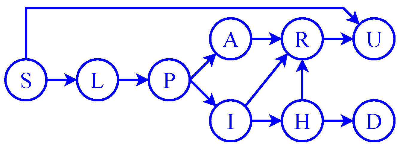
2.1. Transitions between the Phases of the Disease

To capture the spread and the evolution of the COVID-19 epidemic, we considered a modified version of the compartmental model introduced in [21]. This model divides the population of N individuals into eight classes, representing the different stages of the illness. The compartments of the model correspond to the following subsets/groups of the population: susceptible individuals ( S ), infected people in the latent ( L ) and the pre-symptomatic ( P ) phases, infected people in the main sequence of the disease ( A , I ), infected people who need hospital treatment ( H ), and finally, the recovered ( R ) and deceased ( D ) people. The main phase of the disease is further divided into those who remain asymptomatic ( A ) and those who produce symptoms ( I ).
In this work, the model of [21] was complemented with a new compartment ( U ) comprising all individuals who became immune through vaccination. The members of this compartment are governed by the daily number of vaccinated people ( V ). A discrete-time (DT) version of the augmented continuous-time model was obtained through the explicit Euler method with a 1 d-long sampling period. The dynamic equations are given as follows:
{ (1a) S k + 1 = S k β k P k + I k + δ A k S k / N ν S k S k + R k V k , (1b) L k + 1 = L k + β k P k + I k + δ A k S k / N α L k , (1c) P k + 1 = P k + α L k ζ P k , (1d) I k + 1 = I k + γ ζ P k ρ I I k , (1e) A k + 1 = A k + ( 1 γ ) ζ P k ρ A A k , (1f) H k + 1 = H k + ρ I η I k λ H k , (1g) R k + 1 = R k + ρ I ( 1 η ) I k + ρ A A k + ( 1 μ ) λ H k ν R k S k + R k V k , (1h) D k + 1 = D k + μ λ H k , (1i) U k + 1 = U k + ν V k .
The transitions between the compartments are illustrated in Figure 1. It is worth mentioning that the recovered’s compartment R contains the recovered people who are not yet vaccinated. To represent all the recovered people including the vaccinated, we can consider the following additional equation:
R k + 1 ( all ) = R k ( all ) + ρ I ( 1 η ) I k + ρ A A k + ( 1 μ ) λ H k ,
which clearly does not affect the dynamics of other states.
The detailed worldwide [54] and local serological [55] and dynamical [7,20,56,57] analysis results provide estimates for the average lengths of the phases of the illness and the probabilities of transitions between the compartments. These parameters are aligned with the Hungary-specific data and were presented in detail in [21]. After infection, the latent period of the disease ( L ) usually lasts approximately α 1 = 2.5 d. This period is followed by a pre-symptomatic phase ( P ) of ζ 1 = 3 d. A person in the main sequence of the disease ( I or A ) remains infectious for about ρ I 1 = ρ A 1 = 4 d. The empirical probability of producing symptoms in the main sequence is γ = 0.6 ; furthermore, an η = 0.076 portion of the symptomatic cases require hospitalization. The average length of a hospital treatment is λ 1 = 10 d. A hospitalized patient dies with a probability of μ = 0.205 , or recovers. The recovered people are assumed to be immune to reinfection. We assumed that the disease is transmitted by the members of compartments P , A , and I , such that the relative infectiousness of the asymptomatic individuals ( A ) is δ = 0.75 , compared to those who produce symptoms ( I ). The transmission rate β of the disease is the most prominent parameter of the epidemic spread, which is typically time-dependent. The nominal values of the above-mentioned model parameters and their assumed uncertainty are collected in Table 1. For simplicity, each uncertain parameter was assumed to have a normal distribution, such that its nominal value ( μ ) is the expectation and its uncertainty ( ± a % ) gives the 2 σ confidence interval with the standard deviations σ = a μ / 200 .
Here, we examined the evolution of the epidemic in a fixed time window between 1 March 2020 ( k = 0 ) and 30 June 2021 ( k = T ). This interval contains the first three waves of the epidemic in Hungary. Subscript k { 0 , 1 , , T } denotes the number of days elapsed in the given time window of length T + 1 .

2.2. Vaccination Model

For simplicity, our vaccination model assumed that only susceptible and recovered people are eligible for vaccination, and we neglected those rare cases when the shot is given during an unidentified infection. Based on the serological test data [58], our model assumed that a subject becomes immune T v = 21 d after the first dose with an average probability of ν = 0.75 . Correspondingly, variable V k in (1) denotes the number of individuals who received the first dose of vaccine on day k T v . In our model,
an individual is said to be immune to the disease if he/she will not be infected within the modeled time horizon.
With this simplification, the people in the R and U compartments do not transmit the disease any more, as well as those who are still in the hospital. It is worth remarking that a positive IgG test does not necessarily ensure immunity in this sense. Serological tests suggest that even a relatively high IgG level does not exclude the possibility of reinfection [59].
On the other hand, we assumed that the willingness of the susceptible and recovered patients to vaccinate is roughly the same. Namely, the proportion of susceptible and recovered people vaccinated coincides with the proportion of all susceptibles and recovereds on each day. Therefore, the model counts with ν S k V k / ( S k + R k ) susceptible and ν R k V k / ( S k + R k ) recovered individuals who achieved immunity at time k. It is worth remarking that the value of V k is known, but cannot be manipulated as the computations were performed on past data of the epidemic spread. Correspondingly, V : k V k can be considered as a preliminarily known input, or a scheduling variable [60], or a measured disturbance [36,61]. The official European vaccination data including Hungary are available at [62]. Official Hungarian COVID-related data with additional analyses are also available at [63].

2.3. Computing the Reproduction Number

To give meaningful estimates from an epidemiological perspective, we computed the basic and the time-dependent effective reproduction numbers. The basic reproduction number, namely the average number of new infections generated by a single infected individual in a fully susceptible population, can be given by the following closed-form expression [21]:    
R 0 = β 1 ζ + γ ρ I + δ ( 1 γ ) ρ A ,
It must be noted that using R 0 = 2.2 , an early estimate for Hungary commonly used in the literature, and expressing the transmission rate β from the equation, a nominal value of β = 1 / 3 can be given. However, as this parameter is highly influenced by the circumstances varying in time (e.g., the stringency of restrictions, new variants of the virus, etc.), it is considered to be a time-dependent parameter and estimated as such (the corresponding R 0 being calculated afterwards).
The time-dependent effective reproduction number R t shows the average number of infections caused by a single individual, given the state of the model at time t (thus, taking into account the time-varying nature of beta and the decrease of the susceptible population). This is calculated as follows,
R t = β t 1 ζ + γ ρ I + δ ( 1 γ ) ρ A S t N with t { 0 , 1 , , T }
It can be a base for comparison between different epidemic-handling strategies, incorporating the strictness of the restrictions as well. In accordance with the traditional notation “ R t ”, we used t I 0 T (instead of k) as the time parameter of the time-dependent reproduction number.
Inspired by [21], we considered the daily transmission rate β k of the disease an unknown time-dependent parameter. The past values of β k were computed such that the evolution of the epidemic spread matched the available observations.

2.4. Available Measurements

It is commonly stated in the literature [24,25] that the daily number of infected people is not well observable, as the measurement relies on aggressive and exhaustive contact tracing and testing strategies [64,65]. Though it is reasonable to assume that testing is wide-spread and quick enough in the hospitals, the registered numbers of hospitalized patients [66] are still influenced by practical considerations. The limited healthcare capacity on weekends and holidays usually results in a lower number of performed and documented tests, as well as in a delayed hospital discharge. Therefore, following the common engineering practice, we applied a 7 d-long moving average filter to the published data ( H k Off , raw ) [66] to avoid biased estimates caused by these administrative inaccuracies. The smoothed time series H k Off is formally calculated as:
H k Off = 1 min ( 3 , T k ) + min ( 3 , k ) + 1 i = min ( 3 , k ) min ( 3 , T k ) H k + i Off , raw .
Obviously, the 7 d-long sliding window must be truncated at both ends of the series. Finally, the filtered hospitalization data were considered as the single available processed measurement, which reveal relevant information about the time-evolution of the process.

3. Optimization-Based Reconstruction of Past Epidemiological Data

State-Space Model Representation and Problem Statement

In 1, we presented the dynamic Equation (1) of the epidemic spread. We introduced a possible vaccination model in Section 2.2, where V k acts as a measured disturbance input of the dynamical model. In Section 2.3, we explained why parameter β k can be considered as an unknown input of the system. Finally, in Section 2.4, we proposed to consider the hospitalization data ( H ) as the model output. These “ingredients” allowed us to embed the epidemic spread model into the following discrete-time state-space representation:
x k + 1 = f ( x k , u k , θ , v k ) , y k = C x k ,
where x k = ( S k , L k , P k , I k , A k , H k , R k , D k , U k ) R n is the state, u k = β k R m is the unknown input, θ = ( α , ζ , ρ I , ρ A , λ , δ , γ , η , μ , ν ) R p is the vector of model parameters, v k = V k R q is a measured disturbance, and y k = H k R s is the output with C = ( 0 0 0 0 0 1 0 0 0 ) .
In [22], we presented two possible linear time-invariant (LTI) methods to reconstruct the past states x k + 1 and the unknown inputs u k using the measured output y k , k = I 0 T 1 . Both techniques in [22] rely on the dynamic inversion of the LTI subsystem of Model (1). In this paper, we revisited the unknown input filtering problem and reformulated it as an optimal predictive tracking control problem. Namely, we computed an optimal input sequence u k , k = I 0 T 1 such that the output y k of the system follows the reference signal r k = H k Off , which contains the past output measurements, i.e., the daily number of hospitalized patients ( H k Off ). The simultaneous unknown input and state reconstruction can be formulated as the following optimization task.
Problem 1
(NMPC for epidemiological data reconstruction with fixed model parameters). Given the dynamical model (6) with initial condition x 0 , a vector of constants θ, a measured disturbance v k , and a reference output trajectory r k + 1 to track ( k I 0 T 1 ), we looked for a sequence of inputs u k and states x k + 1 that solve the state recursion (6), satisfy the constraint u k U , and minimize the following weighted cost function:
J ( X , U ) = k = 0 T 1 C x k + 1 r k + 1 Q 2 + k = 0 T 2 u k + 1 u k R 2 ,
where X = ( x 1 x T ) and U = ( u 0 u T 1 ) collect the free decision variables of the optimization, Q, R are positive definite weight matrices, and U is a closed subset of the input space  R m .
In Problem 1, we formulated a data assimilation problem in the form of a nonlinear model predictive controller (NMPC) computation. The available numerical optimization tools [40,41,42,43] make it possible to solve Problem 1 precisely in a reasonable time. From an epidemiological point of view, the first term of the cost function (7) minimizes the deviation of the computed number of hospitalized patients from the official data, whereas the second term minimizes the slope of the transmission rate of the pathogen. In this way, the NMPC design provides an optimal smooth solution for the unknown transmission rate function β : { 0 , , T 1 } U = [ 0.06 , 1 ] , which does not have sudden changes.
Remark 1.
The daily transmission rate of the disease β k is an unknown time-dependent (but, supposedly not abruptly varying) parameter. During an outbreak of the epidemic, the number of infected people is not negligible, namely the sum P k + I k + δ A k is significant. In this case, the transmission rate function β : k β k influences the overall dynamics significantly and determines the shape of the epidemic wave. Therefore, parameter β k is generally well identifiable from the measurements during an outbreak of the epidemic, and it becomes uncertain when the number of infectious people is small.
The unknown input filtering task becomes complicated when the model parameters and the initial state (from which the state reconstruction was performed) are probabilistic variables. In the next section, we address the stochastic extension of Problem 1.

4. Statistical Analysis for Normally Distributed Model Parameters

4.1. Gaussian Assumptions

In this section, we allowed the model parameters to vary in time ( θ ^ : k θ ^ k ), but we assumed that the parameter process θ ^ is a collection of independent identically distributed (i.i.d.) Gaussian random variables:
θ ^ k N ( μ θ , Σ θ ) for all k = 0 , 1 , , T 1 ,
where μ θ is the expected value of θ ^ k corresponding to the values presented in 1 and the diagonal Σ θ is its variance. The expected value of the parameter vector contains the nominal values from Table 1, whereas the variances are determined such that the uncertainty intervals from Table 1 resemble the 2 σ confidence intervals. Moreover, we assumed that the initial state, from which the prediction was performed, is itself a random variable, namely:
x ^ 0 N ( μ 0 x , Σ 0 x ) .
Consequently, every further state and output are random variables, which obey the following stochastic recursion and output equation:
x ^ k + 1 = f ( x ^ k , u ^ k , θ ^ k , v k ) , y ^ k = C x ^ k .
Due to the nonlinear terms in the state transition function f, the distribution of the predicted states x ^ k becomes more and more complicated as we look forward in time ( k = 1 , 2 , ) . Therefore, it is very inefficient to compute or at least approximate the non-Gaussian probability density functions of the predicted states for the nonlinear stochastic model (10). As is commonly done in the literature (see, e.g., [50,51,52,53]), we performed a tube-like trajectory estimation. With this technique, each predicted state x ^ k is described by the first two moments, the expected value μ k x , and the variance Σ k x , namely the states are approximated by normal distributions:
x ^ k N ( μ k x , Σ k x ) for all k = 0 , 1 , 2 ,

4.2. Closed-Loop Control Policy

In the literature [44], the values of the optimal control input u are often searched as functions of the states as follows:
u ^ k = μ k u K ( μ k x ) ( x ^ k μ k u ) ,
where μ k u are free decision variables and K is (not necessarily a closed-form) function of the expected state. Thus, the control input is inherently a random variable and is normally distributed as the state (11) itself is approximated by a Gaussian. If Σ k x θ = ( Σ k θ x ) denotes the covariance between x ^ k and θ ^ k , the joint distribution of x ^ k , u ^ k , and θ ^ k is:
( x ^ k u ^ k θ ^ k ) N ( μ k , Σ k ) , where μ k = ( μ k x μ k u μ θ ) , Σ k = ( ) ( Σ k x Σ k x θ Σ k θ x Σ θ ) ( I K ( μ k x ) 0 0 0 I ) .
Remark 2
(Nonlinear state-dependent input policy). When K = 0 , the optimal tracking problem is said to be an open-loop MPC problem [67], whereas K 0 results in a so-called closed-loop MPC problem [51], where the optimal input policy is parameterized by the state. A stabilizing state feedback (12) is typically useful when the predicted states are random variables, and their actual realizations may deviate from the predicted expectations. When the prediction model is stochastic, a sequence of deterministic input values ( K = 0 ) may result in a diverging sequence of state variances, and hence in a conservative (overly cautious) prediction. When the input is parameterized by the state ( K 0 ), the adaptability of the input may reduce the uncertainty of the predicted states significantly if the feedback function (12) is determined appropriately. In this sense, the gain function quantifies the trade-off between the uncertainty of the state and the input. Unfortunately, it is not straightforward to compute a stabilizing gain function K for the nominal model (6). Later, in Section 4.5, we demonstrate that a reference state trajectory (if available) makes it possible to compute the values of K separately in each operating reference state through a classical LTI state feedback approach, e.g., a pole placement or a linear quadratic regulator (LQR) design ([68] Section 6.4.2).

4.3. Probabilistic Cost and Input Constraint

Problem 1 with the stochastic state Equation (10) and the joint distribution (13) results in a stochastic optimal control problem, where both the cost function (7) and the input constraint are probabilistic. Therefore, the inputs and the states are meant to be found such that they minimize the expected cost, namely:
J ( M , S , V ) = k = 0 T 1 C μ k + 1 x r k + 1 Q 2 + k = 0 T 2 μ k + 1 u μ k u R 2 + k = 0 T 1 Tr Q C Σ k + 1 x C + k = 0 T 2 Tr ( R K ( μ k + 1 x ) Σ k + 1 x K ( μ k + 1 x ) ) + k = 0 T 2 Tr ( R K ( μ k x ) Σ k x K ( μ k x ) R He { K ( μ k + 1 x ) Cov ( x ^ k + 1 , x ^ k ) K ( μ k x ) } ) .
where M = ( μ 1 x μ T x ) , S = ( Σ 1 x Σ T x Σ 1 θ x Σ T θ x ) , and V = ( μ 0 u μ T 1 u ) .
The expanded Formula (14) of the expectation of cost (7) is derived in Appendix A.
Remark 3.
The term Cov ( x ^ k + 1 , x ^ k ) = Cov ( f ( x ^ k , u ^ k , v k , θ ^ k ) , x ^ k ) in (14) is typically a non-quadratic function of the mean and the variance of the joint distribution (13). This term introduces a potential difficulty to the optimization, which is addressed later in 18.
The conditions on the input can be formulated as chance constraints of the form Pr ( u ^ k U ) p u , where p u denotes the probability level of the confidence set U . When u ^ k comprise a single input and the input domain U is an interval, the chance constraint Pr ( u ^ k [ u ̲ , u ¯ ] ) p u is equivalent to the following deterministic interval constraint [51]:
μ k u [ u ̲ + c , u ¯ c ] , with c = Φ 1 ( p u + 1 2 ) K ( μ k x ) Σ k x K ( μ k x ) ,
where Φ : R ( 0 , 1 ) denotes the (cumulative) distribution function of the standard normal distribution N ( 0 , 1 ) . This technique for the reformulation of a probabilistic condition is referred to as constraint tightening [69].

4.4. Linear Approximation of the State Dynamics around the Expectation

In the literature, there exist different stochastic sample-based optimization approaches for a predictive optimal controller design; see, e.g., [45,46,47,48,49,50]. However, these approaches are computationally tractable only for a shorter prediction horizon. Alternatively, we have the possibility to formulate deterministic recursions for the first two moments of the state vector, e.g., [51] proposed the state transition function f to be approximated by its first-order Taylor polynomial around the expected values μ k = ( μ k x , μ k u , μ θ ) of the probabilistic variables ( x ^ k , u ^ k , θ ^ k ), namely:
x ^ k + 1 f ( x , u , θ ) ( μ k , v k ) ( x ^ k u ^ k θ ^ k ) + f ( μ k , v k ) f ( x , u , θ ) ( μ k , v k ) μ k .
This approach leads to a deterministic mean-variance (“ μ Σ ”) dynamics, which is typically nonlinear in the free variables μ k x and μ k u .
{ (18a) μ k + 1 x = f ( μ k , v k ) , (18b) Σ k + 1 x θ = f ( x , u , θ ) ( μ k , v k ) ( I K ( μ k x ) 0 0 0 I ) ( Σ k x θ Σ θ ) , (18c) Σ k + 1 x = f ( x , u , θ ) ( μ k , v k ) Σ k ( f ( x , u , θ ) ( μ k , v k ) ) .
Note that the linear Taylor approximation of x ^ k + 1 allowed us to express the non-quadratic term in the cost function (14) as follows:
Cov ( x ^ k + 1 , x ^ k ) = f ( x , u , θ ) ( μ k , v k ) ( I K ( μ k x ) 0 0 0 I ) ( Σ k x θ Σ θ )
The dynamic equations in (18) constitute a possible deterministic prediction model for System (10) and result in the following nonlinear optimal predictive control problem.
Problem 2
( μ Σ -NMPC for unknown-input state reconstruction). Given the dynamical model (18) with an initial state distribution (9), an i.i.d. parameter process (8), a measured disturbance v k , an input policy (12) with a fixed gain function K, and a reference output trajectory r k + 1 to track ( k I 0 T 1 ), we looked for a sequence of deterministic values μ k u , state moments μ k + 1 x , Σ k + 1 x , and covariance matrices Σ k + 1 x θ with Σ 0 x θ = 0 , which solve (18), satisfy the input constraint (16), and minimize the cost (14). The free variables of the optimization are collected in ().
Problem 2 is a stochastic data assimilation problem, reformulated as an optimal predictive tracking problem with a deterministic nonlinear μ Σ -prediction model (10). Henceforth, we refer to Problem 2 as a Gaussian or mean-variance NMPC problem ( μ Σ -NMPC). In general, the variance dynamics (18b,c) significantly increase the complexity of the control problem. If n and p denote the dimension of the state x ^ k and the parameter θ ^ k , respectively, the equations in (18) comprise n p + n ( n + 1 ) / 2 separate scalar equations, whereas the deterministic model (6) constitutes a system of n scalar equations. Therefore, the μ Σ -NMPC in Problem 2 is typically (at least) an order of magnitude more demanding than the ordinary NMPC in Problem 1. However, an appropriate initial guess for the solution of μ Σ -NMPC may reduce the computational complexity of the optimization substantially by providing a fast convergence of the solution.

4.5. Initial Solution for the μ Σ -NMPC Problem

In this section, we compute a pseudo-optimal (i.e., feasible, but not necessarily optimal) solution of Problem 2, which satisfies the dynamic equations (10) and the input constraint (16), but it does not necessarily minimize the cost (14). The computed solution can be considered an initial value for the μ Σ -NMPC problem. The solution relies on three observations.
First, observe that the mean equation in (18a) resembles the deterministic state recursion in (6) as the mean dynamics is not affected by the variances nor the state-dependent feedback gain K ( μ k x ) . Therefore, Problem 2 simplifies to Problem 1 if we neglect the variances ( S = 0 ) and their dynamics (18b,c) from the optimization. Accordingly, a possible guess for the expectation ( M , V ) , which solves the mean Equation (18a), can be given by the optimal solution ( X * , U * ) of Problem 1 with initial condition x 0 μ 0 x and parameter vector θ μ θ .
Secondly, we note that the gain function K depends (by design) on the expected states only. This allows computing an appropriate gain K k at each operating point x 0 * = μ 0 x , x k * , k I 1 T 1 along the computed mean solution. We determined K k through the DT version of the LQR design applied to the controllable modes of the pair ( A k , B k ) , where:
A k = f x ( μ k , v k ) , B k = f u ( μ k , v k ) .
Through a sequence of DT-LQR computations, we selected a static feedback gain matrix K k at each time instant k, which minimizes the quadratic cost:
t = k ( x t Q k l q r x t + u t R k l q r u t ) , with u t = K k x t .
For a DT-LTI state-space model x t + 1 = A k x t + B k u t (with t = 0 , 1 , 2 , , but a fixed k), the constant gain matrix K k can be computed through simple linear algebra operations ([68] Section 6.4.2), which were implemented in function dlqr of the Control System Toolbox [70] for MATLAB. When selecting the weight matrices Q k l q r and R k l q r of the LQR problem at time k I 0 T 1 , we needed to take into consideration that the value of K k quantifies the trade-off between the uncertainty of x ^ k + 1 and u ^ k . If the locally stabilizing gain has a higher value, the input u ^ k is more adaptive (hence, more uncertain), but the uncertainty of x ^ k + 1 is smaller. However, the chance constraint (16) does not allow the uncertainty of u ^ k to increase beyond any bounds. Therefore, the gain should be selected carefully, such that it generates an input distribution satisfying (16). If the first computed value for K k does not result in an admissible input distribution, we are allowed to compute K k multiple times with a gradually decreasing value for R k l q r .
Finally, with the knowledge of μ k , v k , K ( μ k x ) = K k , k I 0 T 1 , Σ 0 x , and Σ 0 x θ = 0 , we computed the variances according to (18b,c), which give the value of S in (15). If the expected values and K are fixed, the variances are well-defined by the variance Equation (18b,c). By construction, the tuple ( M , S , V ) is a feasible solution for Problem 2 as it satisfies both the μ Σ -Equation (18) and the input constraint (16). The computed solution is a good initial guess for the optimal solution of Problem 2. In Algorithm 10, we summarize the proposed operations with a single input u k R and a simple LQR weight selection.
Algorithm 1 Computing a pseudo-optimal solution for Problem 2.
1:
Fix x ^ 0 N ( μ 0 x , Σ 0 x ) , Σ 0 x θ 0 , μ θ , and Σ θ . (Optionally, fix μ 0 u .)
2:
Collect data v k and r k + 1 , then solve Problem 1 to obtain μ k x and μ k u , where k I 0 T 1 .
3:
for   k I 0 T 1 do
4:
     i 1 .
5:
    repeat
6:
        Compute K k for the pair ( A k , B k ) given in (20) through a DT-LQR design
7:
with weight matrices Q l q r I n and R k l q r 2 i 1       i i + 1 .
8:
    until condition (16) is met. (If no such K k is found, let K k 0 .)
9:
    Compute Σ k + 1 x θ , Σ k + 1 x , as given in (18b) and (18c), respectively, using K ( μ k x ) = K k .
10:
end for
Remark 4.
From the authors’ experience, the computationally demanding μ Σ -NMPC optimization for Model (1) will generally not result in a significantly lower expected cost (14) compared to the computed pseudo-optimal solution ( M , S , V ) .

5. Results and Discussion

In this section, we present the numerical results we obtained through the MPC-based reconstruction of the unknown epidemiological data. The results were computed in the MATLAB environment with the Control System Toolbox [70]. For algorithmic differentiation, we used CasADi [40,41]. To solve nonlinear MPC problems, we used IPOPT [42], an interior point line search algorithm, with the MUltifrontal Massively Parallel sparse direct Solver (MUMPS) [71,72]. The MPC implementations are available online in the public repository [73].
To compute the unknown epidemiological data, we followed the operations of Algorithm 10 to find a pseudo-optimal solution for the μ Σ -NMPC in Problem 2. On 1 March 2020 ( k = 0 ) , we assumed a susceptible and almost healthy population, with a small uncertainty as follows:
μ 0 x = ( N 40 10 10 10 10 0 0 0 0 ) , Σ 0 x = diag ( 7 , 1 , 1 , 1 , 1 , 1 , 1 , 1 , 0 ) .
We note that the effect of the initial number of infected people on the reconstructed state vanishes after a transient period due to the stability properties of the compartmental model (1). Furthermore, we considered pairwise independent random parameters with μ θ and a diagonal Σ θ as presented in Table 1. We fixed the initial value for β to μ 0 u = 1 / 3 [21]. We solved the ordinary NMPC in Problem 1 to find the candidate mean functions for x ^ and u ^ . Then, we computed the gain matrices and the variances of the joint distribution (13). Using the obtained feasible solution as an initial guess, we solved the μ Σ -NMPC in Problem 2. We learned that the local optimum ( M * , S * , V * ) found for Problem 2 is qualitatively the same as the initial guess ( M , S , V ) . The relative difference in the cost obtained by the optimal and the pseudo-optimal solution is negligible, namely:
J ( M , S , V ) J ( M * , S * , V * ) J ( M * , S * , V * ) 7.1 × 10 7 , where J ( M * , S * , V * ) 17 , 075.129 .
If X , X * R ( n + m + n p + n ( n + 1 ) / 2 ) · T 1 denote the vectors of independent variables of ( M , S , V ) and ( M * , S * , V * ) , respectively, the relative difference between X and X * is:
X X * / X * 2.86 × 10 11 , where X * 3.1978 × 10 11 .
In Table 2, we present the dimensional differences between the ordinary NMPC and the μ Σ -NMPC if the length of time window is T = 487 d. In Figure 2, we illustrate the computed marginal distributions of the transmission rate of the pathogen and the daily numbers of people in the different stages of the disease. The expectation for the states are presented in Plot 1 of Figure 2, which were computed through the ordinary NMPC design in Problem 1. In each of Plots 2–12 of Figure 2 and Figure 3, the time evolution of the marginal distributions of scalar quantities are visualized, such that the shaded dark and light areas highlight the 1 σ and 1 σ confidence intervals, respectively. The shape of the epidemic curves clearly show the three waves of the epidemic until summer 2021.
As was noted in Remark 1, the daily transmission rate becomes uncertain when the number of infectious people reduces significantly. In this case, the input constraint with the computed gain K k may be violated; therefore, we increased the input weight R k l q r to obtain a lower gain K k . These heuristic operations to compute an admissible gain were relevant only when the third wave of the epidemic suddenly dropped after the end of April 2021. The scaled logarithm of the input weights on each day k are illustrated in Plot 2 of Figure 2. In Plot 3 of Figure 2, we present the reconstructed number of hospitalized patients in comparison with the official (i.e., reference) data. Plots 4, 5, and 6 of Figure 2 illustrate three derived probabilistic quantities z ^ k = h ( x ^ k , u ^ k , θ ^ ) , namely the time-dependent effective reproduction number (4) ( [ z ^ k ] 1 = R k ), the number of all infected people ( [ z ^ k ] 2 = L ^ k + P ^ k + I ^ k + A ^ k + H ^ k ), and the number of daily new infections ( [ z ^ k ] 3 = β ^ k ( P ^ k + I ^ k + δ ^ A ^ k ) S ^ k N ). The first and third coordinates of z ^ k are nonlinear functions of random variables. Therefore, the mean and the variance of z ^ k were approximated by the first-order Taylor polynomial of function h, namely,
z ^ k h ( x , u , θ ) ( μ k ) ( x ^ k u ^ k θ ^ k ) + h ( μ k ) h ( x , u , θ ) ( μ k ) μ k N ( h ( μ k ) , h ( x , u , θ ) ( μ k ) Σ k ( h ( x , u , θ ) ( μ k ) ) ) .
The yellow curve in Plot 4 illustrates the estimated reproduction number published online by Atlo Team in [74].
In Plot 12 of Figure 3, we present three uncertain time series, namely the number of recovered, but not yet vaccinated people (blue), the cumulative number of recovered people (red), and the cumulative number of immune people (green).
In Figure 2 and Figure 3, we can observe the successfully suppressed first wave with a dramatic effect of the strict lockdown introduced in March 2020. As a result, the disease was mainly confined to closed institutions such as certain hospital wards and elderly homes. This policy could not be maintained in the autumn of 2020, and therefore, a substantially larger second wave occurred, causing a huge burden on the healthcare system. Therefore, further restrictions (online education in secondary schools, closure of certain public spaces, banning of most gatherings, and curfew from 8 p.m. to 5 a.m.) had to be introduced in the first half of November 2020. These measures had the planned effect in terms of the significant reduction of the transmission rate, as is visible in Plot 2 of Figure 3. Then, from January 2021, R t began to increase again due to the appearance of the more contagious alpha (B.1.1.7) variant, although all of the former restrictions remained in effect. The alpha variant caused the largest peak of the epidemic so far in the spring of 2021 with a maximum of 12,553 hospitalized people on 30 March 2021. Further restrictions had to be introduced on 8 March 2021, where the main component was the closing of all schools. Together with the intensive vaccination in the first half of 2021, this made the decrease in the number of infected people definitely fast. The ratio of the peaks of the estimated β in February 2021 and December 2020 was approximately 1.62, which matches well with literature reports (1.4–1.8) in the U.K. [75]. We note that we can compare these data since they were estimated under the same restriction level. Plot 12 in Figure 3 shows the estimated number of people gaining immunity by infection and/or vaccination. According to this estimation, more than 30% of the population might have gone through the COVID infection until the end of June 2021. This suggests an approximately 26% detection rate. This is significantly lower than the value of certain European countries such as Germany, Italy, or Spain, reaching or sometimes exceeding 50%, but the number of performed tests per population has also been much lower in Hungary than in the mentioned countries [76].

6. Conclusions

In this paper, we proposed an optimization-based data assimilation approach to compute the unknown inputs and states of discrete-time compartmental epidemic models with uncertain normally distributed parameters. We started from the assumption that the joint state input parameter distribution is Gaussian. Then, a deterministic mean-variance recursion was developed, which made it possible to formulate the stochastic data assimilation problem as a single model predictive control design with a nonlinear mean-variance prediction model. We noted and demonstrated that the resulting μ Σ -NMPC is computationally intensive, but its local optimum can be well approximated by a more efficient ordinary NMPC and further closed-form variance computations.
We proposed simple heuristics to predict appropriate feedback gains, which realize state-dependent control actions along the prediction horizon. In this way, a trade-off can be made between the uncertainty of the computed states and inputs as the predicted control action is scheduled by the deviation between the actual realization of the state and its predicted expectation. As the approach does not make a difference between the unknown parameters and inputs, the joint state observation, change detection, and parameter estimation are also possible.
Through the finite horizon predictive control computation, we estimated the unknown data of the past evolution of the COVID-19 epidemic spread within a fixed time window in Hungary. Among the unknown quantities, we considered the daily number of people in the different phases of the disease and the transmission rate of the pathogen, which highly depends on the actual social distancing rules, mobility restrictions, and virus mutations. The unknown time series were computed such that the expected value of the computed number of hospitalized patients fit the truly observed data as much as possible. Compared to our previous results [21,22], we considered an augmented and uncertain compartmental epidemiological model with normally distributed random model parameters and a simple vaccination model as well.
The main limitations of this study were the following. The length of hospital treatment was considered to be constant in the model, since no data have been published on the daily new hospital admissions with COVID-19, from which this parameter could be tracked efficiently. Moreover, no representative nationwide serological testing in Hungary has been organized since the summer of 2020. Such a result would definitely be helpful in making the estimate on the number of immune people more precise. Finally, the waning of immunity after infection or vaccination was also not taken into consideration in the model. However, such an extension does not affect the applicability of the proposed MPC-based estimation.
With a few modifications, the approach can be applied to compute multiple uncertain possibly time-dependent parameters, but also for the prediction of the future behavior of the epidemic spread. The proposed methodology is able to extract and reconstruct detailed information from the whole time horizon of the epidemic process beyond giving estimates for the cumulative number of infected and recovered people. Future work will be focused on the analysis of other European countries.

Author Contributions

Conceptualization, G.S. and P.P.; methodology, P.P. and G.S.; formal analysis, P.P. and B.C.; software, B.C. and P.P.; visualization, B.C. and P.P.; writing—review and editing, P.P. and B.C.; supervision, G.S.; funding acquisition, G.S.; project administration, G.S. All authors have read and agreed to the published version of the manuscript.

Funding

This work was supported by the grants “OTKA” SNN125739 and K131545 and the Thematic Excellence Program (TKP2020-NKA-11) of the National Research, Development, and Innovation (NRDI) Office. We also acknowledge the partial support of the Ministry for Innovation and Technology and the NRDI Office within the framework of the Autonomous Systems National Laboratory and the Epidemic Dynamics, Invasion Ecology, and Data-driven Health National Laboratory Programs.

Institutional Review Board Statement

Not applicable.

Informed Consent Statement

Not applicable.

Data Availability Statement

The MPC implementation together with the collected hospitalization [66] and vaccination data [63] are all available online in the public repository [73].

Acknowledgments

P.P. is grateful to Roland Tóth and Tamás Péni for the useful discussions on the theory and computational aspects of stochastic and/or nonlinear MPC problems. We are also very thankful to Krisztina Latkóczy for the inspiring conversations about the microbial background of the ongoing COVID-19 pandemic.

Conflicts of Interest

The authors declare no conflict of interest.

Abbreviations

The following abbreviations are used in this manuscript:
SEIRSusceptible–exposed–infected–recovered (compartmental model)
IgGImmunoglobulin G
CTContinuous-time
DTDiscrete-time
ODEOrdinary differential equation
i.i.d.Independent identically distributed
LTILinear time-invariant
MPCModel predictive controller
NMPCNonlinear model predictive controller
SNMPCStochastic nonlinear model predictive controller
LQRLinear quadratic regulator
μ Σ -…Mean-variance equations/dynamics/recursion/prediction model/NMPC
μ Σ -NMPCMean-variance nonlinear model predictive controller

Appendix A

In this section, we prove that the expected value of the cost:
(borrowed from (7)) J ( X , U ) = k = 0 T 1 C x ^ k + 1 r k + 1 Q 2 + k = 0 T 2 u ^ k + 1 u ^ k R 2 ,
can be expressed as:
J ( M , S , V ) = k = 0 T 1 C μ k + 1 x r k + 1 Q 2 + k = 0 T 2 μ k + 1 u μ k u R 2 (borrowed from (14)) + k = 0 T 1 Tr Q C Σ k + 1 x C + k = 0 T 2 Tr ( R K ( μ k + 1 x ) Σ k + 1 x K ( μ k + 1 x ) ) + k = 0 T 2 Tr ( R K ( μ k x ) Σ k x K ( μ k x ) R He { K ( μ k + 1 x ) Cov ( x ^ k + 1 , x ^ k ) K ( μ k x ) } ) .
The proof is given in multiple steps, but it is essentially based on a simple observation, which allows expressing the expectation of the squared weighted norm of a random variable x ^ as follows:
E ( x ^ Q 2 ) = μ x Q 2 + Tr ( Q Σ x )
To prove (A1), first, consider the following chain of identities:
Q Σ x = Q Var ( x ^ ) = Cov ( Q x ^ , x ^ ) = E ( Q x ^ x ^ ) Q μ x ( μ x ) .
Then, we take the trace of the quantities in (A2) to obtain:
Tr ( Q Σ x ) = E ( x ^ Q x ^ ) ( μ x ) Q μ x .
Equality (A1) is a direct consequence of (A3). Accordingly, the squared weighted norm of the output error at time k + 1 can be expressed as follows:
C x ^ k + 1 r k + 1 Q 2 = C μ k + 1 x r k + 1 Q 2 + Tr ( Q C Σ k + 1 x C ) .
Secondly, the input variation cost is expressed as follows:
E ( u ^ k + 1 u ^ k R 2 ) = μ k + 1 u μ k u R 2 + Tr ( R Var ( u ^ k + 1 u ^ k ) ) .
The variance term in (A5) is further developed as follows:
Var ( u ^ k + 1 u ^ k ) = Var ( u ^ k + 1 K ( μ k + 1 x ) ( x ^ k + 1 μ k + 1 x ) u ^ k + K ( μ k x ) ( x ^ k μ k x ) )
= Var ( K ( μ k + 1 x ) x ^ k + 1 K ( μ k x ) x ^ k ) = Var ( K ( μ k + 1 x ) x ^ k + 1 ) + Var ( K ( μ k x ) x ^ k )
He { Cov ( K ( μ k + 1 x ) x ^ k + 1 , K ( μ k x ) x ^ k ) } = K ( μ k + 1 x ) Σ k + 1 x K ( μ k + 1 x ) + K ( μ k x ) Σ k x K ( μ k x )
He { K ( μ k + 1 x ) Cov ( x ^ k + 1 , x ^ k ) K ( μ k x ) }
Finally, the output error (A4) and the input variation error (A5) with the variance expression (A9) give the expected value (14) of the random cost (7).

References

  1. Miller, I.F.; Becker, A.D.; Grenfell, B.T.; Metcalf, C.J.E. Disease and healthcare burden of COVID-19 in the United States. Nat. Med. 2020, 26, 1212–1217. [Google Scholar] [CrossRef] [PubMed]
  2. Baker, S.R.; Bloom, N.; Davis, S.J.; Terry, S.J. COVID-Induced Economic Uncertainty; Technical Report; National Bureau of Economic Research: Cambridge, MA, USA, 2020. [Google Scholar] [CrossRef]
  3. Cao, L.; Liu, Q.; Hou, W. COVID-19 modeling: A review. arXiv 2021, arXiv:2104.12556. [Google Scholar]
  4. Shinde, G.R.; Kalamkar, A.B.; Mahalle, P.N.; Dey, N.; Chaki, J.; Hassanien, A.E. Forecasting models for coronavirus disease (COVID-19): A survey of the state-of-the-art. SN Comput. Sci. 2020, 1, 197. [Google Scholar] [CrossRef] [PubMed]
  5. Biswas, M.H.A.; Paiva, L.T.; de Pinho, M. A SEIR model for control of infectious diseases with constraints. Math. Biosci. Eng. 2014, 11, 761–784. [Google Scholar] [CrossRef]
  6. Brauer, F. Compartmental models in epidemiology. In Mathematical Epidemiology; Springer: Berlin/Heidelberg, Germany, 2008; pp. 19–79. [Google Scholar] [CrossRef]
  7. He, S.; Peng, Y.; Sun, K. SEIR modeling of the COVID-19 and its dynamics. Nonlinear Dyn. 2020, 101, 1667–1680. [Google Scholar] [CrossRef] [PubMed]
  8. Röst, G.; Bartha, F.A.; Bogya, N.; Boldog, P.; Dénes, A.; Ferenci, T.; Horváth, K.J.; Juhász, A.; Nagy, C.; Tekeli, T.; et al. Early phase of the COVID-19 outbreak in Hungary and post-lockdown scenarios. Viruses 2020, 12, 708. [Google Scholar] [CrossRef]
  9. Rajabi, A.; Mantzaris, A.V.; Mutlu, E.C.; Garibay, O.O. Investigating dynamics of COVID-19 spread and containment with agent-based modeling. Appl. Sci. 2021, 11, 5367. [Google Scholar] [CrossRef]
  10. Reguly, I.Z.; Csercsik, D.; Juhasz, J.; Tornai, K.; Bujtar, Z.; Horvath, G.; Keomley-Horvath, B.; Kos, T.; Cserey, G.; Ivan, K.; et al. Microsimulation based quantitative analysis of COVID-19 management strategies. PLoS Comput. Biol. 2022, 18, 1–14. [Google Scholar] [CrossRef]
  11. Rzadkowski, G.; Figlia, G. Logistic wavelets and their application to model the spread of COVID-19 pandemic. Appl. Sci. 2021, 11, 8147. [Google Scholar] [CrossRef]
  12. Lalmuanawma, S.; Hussain, J.; Chhakchhuak, L. Applications of machine learning and artificial intelligence for COVID-19 (SARS-CoV-2) pandemic: A review. Chaos Solitons Fractals 2020, 139, 110059. [Google Scholar] [CrossRef] [PubMed]
  13. Satu, M.; Howlader, K.C.; Mahmud, M.; Kaiser, M.S.; Shariful Islam, S.M.; Quinn, J.M.W.; Alyami, S.A.; Moni, M.A. Short-term prediction of COVID-19 cases using machine learning models. Appl. Sci. 2021, 11, 4266. [Google Scholar] [CrossRef]
  14. Ghafouri-Fard, S.; Mohammad-Rahimi, H.; Motie, P.; Minabi, M.; Taheri, M.; Nateghinia, S. Application of machine learning in the prediction of COVID-19 daily new cases: A scoping review. Heliyon 2021, 7, e08143. [Google Scholar] [CrossRef] [PubMed]
  15. Gostic, K.M.; McGough, L.; Baskerville, E.B.; Abbott, S.; Joshi, K.; Tedijanto, C.; Kahn, R.; Niehus, R.; Hay, J.A.; De Salazar, P.M.; et al. Practical considerations for measuring the effective reproductive number, Rt. PLoS Comput. Biol. 2020, 16, e1008409. [Google Scholar] [CrossRef] [PubMed]
  16. Fraser, C. Estimating individual and household reproduction numbers in an emerging epidemic. PLoS ONE 2007, 2, e758. [Google Scholar] [CrossRef] [PubMed]
  17. Cori, A.; Ferguson, N.M.; Fraser, C.; Cauchemez, S. A new framework and software to estimate time-varying reproduction numbers during epidemics. Am. J. Epidemiol. 2013, 178, 1505–1512. [Google Scholar] [CrossRef] [Green Version]
  18. Kucharski, A.J.; Russell, T.W.; Diamond, C.; Liu, Y.; Edmunds, J.; Funk, S.; Eggo, R.M.; Sun, F.; Jit, M.; Munday, J.D.; et al. Early dynamics of transmission and control of COVID-19: A mathematical modelling study. Lancet Infect. Dis. 2020, 20, 553–558. [Google Scholar] [CrossRef] [Green Version]
  19. Koyama, S.; Horie, T.; Shinomoto, S. Estimating the time-varying reproduction number of COVID-19 with a state-space method. PLoS Comput. Biol. 2021, 17, e1008679. [Google Scholar] [CrossRef] [PubMed]
  20. Tsay, C.; Lejarza, F.; Stadtherr, M.A.; Baldea, M. Modeling, state estimation, and optimal control for the US COVID-19 outbreak. Sci. Rep. 2020, 10, 10711. [Google Scholar] [CrossRef] [PubMed]
  21. Péni, T.; Csutak, B.; Szederkényi, G.; Röst, G. Nonlinear model predictive control with logic constraints for COVID-19 management. Nonlinear Dyn. 2020, 102, 1965–1986. [Google Scholar] [CrossRef] [PubMed]
  22. Csutak, B.; Polcz, P.; Szederkényi, G. Computation of COVID-19 epidemiological data in Hungary using dynamic model inversion. In Proceedings of the 15th IEEE International Symposium on Applied Computational Intelligence and Informatics (SACI 2021), Timișoara, Romania, 19–21 May 2021; pp. 91–96. [Google Scholar] [CrossRef]
  23. Sereno, J.; D’Jorge, A.; Ferramosca, A.; Hernandez-Vargas, E.; González, A. Model predictive control for optimal social distancing in a type SIR-switched model. IFAC-PapersOnLine 2021, 54, 251–256. [Google Scholar] [CrossRef]
  24. Phipps, S.J.; Grafton, R.Q.; Kompas, T. Robust estimates of the true (population) infection rate for COVID-19: A backcasting approach. R. Soc. Open Sci. 2020, 7, 200909. [Google Scholar] [CrossRef]
  25. Rocchetti, I.; Böhning, D.; Holling, H.; Maruotti, A. Estimating the size of undetected cases of the COVID-19 outbreak in Europe: An upper bound estimator. Epidemiol. Methods 2020, 9, 20200024. [Google Scholar] [CrossRef]
  26. Bartha, F.A.; Karsai, J.; Tekeli, T.; Röst, G. Symptom-based testing in a compartmental model of COVID-19. In Analysis of Infectious Disease Problems (COVID-19) and Their Global Impact; Springer: Berlin/Heidelberg, Germany, 2021; pp. 357–376. [Google Scholar] [CrossRef]
  27. Lemaitre, J.C.; Perez-Saez, J.; Azman, A.; Rinaldo, A.; Fellay, J. Assessing the impact of non-pharmaceutical interventions on SARS-CoV-2 transmission in Switzerland. Swiss Med. Wkly. 2020, 150, w20295. [Google Scholar] [CrossRef]
  28. Allgöwer, F.; Zheng, A. (Eds.) Nonlinear Model Predictive Control, 1st ed.; Progress in Systems and Control Theory 26; Birkhäuser Basel: Basel, Switzerland, 2000. [Google Scholar] [CrossRef]
  29. Apte, A.; Jones, C.K.R.T.; Stuart, A.M.; Voss, J. Data assimilation: Mathematical and statistical perspectives. Int. J. Numer. Methods Fluids 2008, 56, 1033–1046. [Google Scholar] [CrossRef]
  30. Bröcker, J. On variational data assimilation in continuous time. Q. J. R. Meteorol. Soc. 2010, 136, 1906–1919. [Google Scholar] [CrossRef] [Green Version]
  31. Schumann-Bischoff, J.; Parlitz, U.; Abarbanel, H.D.I.; Kostuk, M.; Rey, D.; Eldridge, M.; Luther, S. Basin structure of optimization based state and parameter estimation. Chaos Interdiscip. J. Nonlinear Sci. 2015, 25, 053108. [Google Scholar] [CrossRef] [Green Version]
  32. Schumann-Bischoff, J.; Parlitz, U. State and parameter estimation using unconstrained optimization. Phys. Rev. E 2011, 84, 056214. [Google Scholar] [CrossRef] [PubMed]
  33. Chen, T.; Kirkby, N.F.; Jena, R. Optimal dosing of cancer chemotherapy using model predictive control and moving horizon state/parameter estimation. Comput. Methods Programs Biomed. 2012, 108, 973–983. [Google Scholar] [CrossRef]
  34. Das, A. Chance-constrained optimization-based parameter estimation for Muskingum models. J. Irrig. Drain. Eng. 2007, 133, 487–494. [Google Scholar] [CrossRef]
  35. Das, A. Parameter estimation for Muskingum models. J. Irrig. Drain. Eng. 2004, 130, 140–147. [Google Scholar] [CrossRef]
  36. Al-Hemeary, N.; Polcz, P.; Szederkényi, G. Optimal solar panel area computation and temperature tracking for a cubesat system using model predictive control. SPIIRAS Proc. 2020, 19, 564–593. [Google Scholar] [CrossRef]
  37. Courtier, P.; Talagrand, O. Variational assimilation of meteorological observations with the direct and adjoint shallow-water equations. Tellus A Dyn. Meteorol. Oceanogr. 1990, 42, 531–549. [Google Scholar] [CrossRef] [Green Version]
  38. Blackmore, L.; Açıkmeşe, B.; Carson, J.M. Lossless convexification of control constraints for a class of nonlinear optimal control problems. Syst. Control Lett. 2012, 61, 863–870. [Google Scholar] [CrossRef]
  39. Mao, Y.; Szmuk, M.; Açıkmeşe, B. Successive convexification of non-convex optimal control problems and its convergence properties. In Proceedings of the 2016 IEEE 55th Conference on Decision and Control (CDC), Las Vegas, NV, USA, 12–14 December 2016; pp. 3636–3641. [Google Scholar] [CrossRef] [Green Version]
  40. Andersson, J.; Gillis, J.; Diehl, M. User Documentation for CasADi v3.4.4. 2018. Available online: http://casadi.sourceforge.net/v3.4.4/users_guide/casadi-users_guide.pdf (accessed on 17 December 2021).
  41. Andersson, J.A.E.; Gillis, J.; Horn, G.; Rawlings, J.B.; Diehl, M. CasADi: A software framework for nonlinear optimization and optimal control. Math. Program. Comput. 2018, 11, 1–36. [Google Scholar] [CrossRef]
  42. Wächter, A.; Biegler, L.T. On the implementation of an interior-point filter line-search algorithm for large-scale nonlinear programming. Math. Program. 2005, 106, 25–57. [Google Scholar] [CrossRef]
  43. Zanelli, A.; Domahidi, A.; Jerez, J.; Morari, M. Forces NLP: An efficient implementation of interior-point methods for multistage nonlinear nonconvex programs. Int. J. Control 2017, 93, 13–29. [Google Scholar] [CrossRef]
  44. Mesbah, A. Stochastic model predictive control: An overview and perspectives for future research. IEEE Control. Syst. Mag. 2016, 36, 30–44. [Google Scholar] [CrossRef] [Green Version]
  45. de la Penad, D.; Bemporad, A.; Alamo, T. Stochastic programming applied to model predictive control. In Proceedings of the 44th IEEE Conference on Decision and Control, Seville, Spain, 15 December 2005; pp. 1361–1366. [Google Scholar] [CrossRef]
  46. Bernardini, D.; Bemporad, A. Stabilizing model predictive control of stochastic constrained linear systems. IEEE Trans. Autom. Control 2012, 57, 1468–1480. [Google Scholar] [CrossRef] [Green Version]
  47. Thangavel, S.; Paulen, R.; Engell, S. Robust multi-stage nonlinear model predictive control using sigma points. Processes 2020, 8, 851. [Google Scholar] [CrossRef]
  48. Thangavel, S.; Paulen, R.; Engell, S. Dual multi-stage NMPC using sigma point principles. IFAC-PapersOnLine 2020, 53, 11243–11250. [Google Scholar] [CrossRef]
  49. Bonzanini, A.D.; Paulson, J.A.; Makrygiorgos, G.; Mesbah, A. Fast approximate learning-based multistage nonlinear model predictive control using Gaussian processes and deep neural networks. Comput. Chem. Eng. 2021, 145, 107174. [Google Scholar] [CrossRef]
  50. Ostafew, C.J.; Schoellig, A.P.; Barfoot, T.D. Conservative to confident: Treating uncertainty robustly within learning-based control. In Proceedings of the 2015 IEEE International Conference on Robotics and Automation (ICRA), Seattle, WA, USA, 26–30 May 2015; pp. 421–427. [Google Scholar] [CrossRef]
  51. Hewing, L.; Kabzan, J.; Zeilinger, M.N. Cautious model predictive control using Gaussian process regression. IEEE Trans. Control. Syst. Technol. 2020, 28, 2736–2743. [Google Scholar] [CrossRef] [Green Version]
  52. Candela, J.Q.; Girard, A.; Rasmussen, C.E. Prediction at an Uncertain Input for Gaussian Processes and Relevance Vector Machines Application to Multiple-Step Ahead Time-Series Forecasting; Technical Report IMM-2003-18; Technical University of Denmark: Kgs. Lyngby, Denmark, 2003. [Google Scholar]
  53. Deisenroth, M.P. Efficient Reinforcement Learning Using Gaussian Processes—Revised Version. Ph.D. Thesis, Faculty of Informatics, Institute for Anthropomatics, Intelligent Sensor-Actuator-Systems Laboratory (ISAS), Karlsruhe, Germany, 2017. [Google Scholar]
  54. de Moura, D.T.H.; McCarty, T.R.; Ribeiro, I.B.; Funari, M.P.; de Oliveira, P.V.A.G.; de Miranda Neto, A.A.; do Monte Júnior, E.S.; Tustumi, F.; Bernardo, W.M.; de Moura, E.G.H.; et al. Diagnostic characteristics of serological-based COVID-19 testing: A systematic review and meta-analysis. Clinics 2020, 75, e2212. [Google Scholar] [CrossRef] [PubMed]
  55. Merkely, B.; Szabó, A.J.; Kosztin, A.; Berényi, E.; Sebestyén, A.; Lengyel, C.; Merkely, G.; Karády, J.; Várkonyi, I.; Papp, C.; et al. Novel coronavirus epidemic in the Hungarian population, a cross-sectional nationwide survey to support the exit policy in Hungary. GeroScience 2020, 42, 1063–1074. [Google Scholar] [CrossRef]
  56. Sedaghat, A.; Oloomi, S.A.A.; Malayer, M.A.; Band, S.; Mosavi, A.; Nadai, L. Modeling and sensitivity analysis of coronavirus disease (COVID-19) outbreak prediction. In Proceedings of the 2020 IEEE 3rd International Conference and Workshop in Óbuda on Electrical and Power Engineering (CANDO-EPE), Budapest, Hungary, 18–19 November 2020; pp. 000261–000266. [Google Scholar] [CrossRef]
  57. Sedaghat, A.; Oloomi, S.A.A.; Malayer, M.A.; Band, S.; Rezaei, N.; Mosavi, A.; Nadai, L. Coronavirus (COVID-19) outbreak prediction using epidemiological models of Richards Gompertz Logistic Ratkowsky and SIRD. In Proceedings of the 2020 IEEE 3rd International Conference and Workshop in Óbuda on Electrical and Power Engineering (CANDO-EPE), Budapest, Hungary, 18–19 November 2020; pp. 000289–000298. [Google Scholar] [CrossRef]
  58. Tartof, S.Y.; Slezak, J.M.; Fischer, H.; Hong, V.; Ackerson, B.K.; Ranasinghe, O.N.; Frankland, T.B.; Ogun, O.A.; Zamparo, J.M.; Gray, S.; et al. Effectiveness of mRNA BNT162b2 COVID-19 vaccine up to 6 months in a large integrated health system in the USA: A retrospective cohort study. Lancet 2021, 398, 1407–1416. [Google Scholar] [CrossRef]
  59. Hu, X.; Lindquist, A. Geometric Control Theory; Royal Institute of Technology: Stockholm, Sweden, 2012. [Google Scholar]
  60. González Cisneros, P.S.; Werner, H. Nonlinear model predictive control for models in quasi-linear parameter varying form. Int. J. Robust Nonlinear Control 2020, 30, 3945–3959. [Google Scholar] [CrossRef]
  61. Bemporad, A.; Ricker, N.L.; Morari, M.; Model Predictive Control Toolbox™User’s Guide (R2019b). MathWorks. 2019. Available online: https://www.mathworks.com/help/pdf_doc/mpc/mpc_ug.pdf (accessed on 17 December 2021).
  62. Data on COVID-19 Vaccination in the EU/EEA. Available online: https://www.ecdc.europa.eu/en/publications-data/data-covid-19-vaccination-eu-eea (accessed on 17 December 2021).
  63. Atlo Team. Koronamonitor: Hungarian Status of Coronavirus Vaccination. 2021. Available online: https://atlo.team/vakcinacio (accessed on 11 November 2021).
  64. Salath, M.; Althaus, C.L.; Neher, R.; Stringhini, S.; Hodcroft, E.; Fellay, J.; Zwahlen, M.; Senti, G.; Battegay, M.; Wilder-Smith, A.; et al. COVID-19 epidemic in switzerland: On the importance of testing, contact tracing and isolation. Swiss Med. Wkly. 2020. [Google Scholar] [CrossRef]
  65. Steinbrook, R. Contact tracing, testing, and control of COVID-19—Learning from Taiwan. JAMA Intern. Med. 2020, 180, 1163–1164. [Google Scholar] [CrossRef]
  66. Data on Hospital and ICU Admission Rates and Current Occupancy for COVID-19. 2021. Available online: https://www.ecdc.europa.eu/en/publications-data/download-data-hospital-and-icu-admission-rates-and-current-occupancy-covid-19 (accessed on 11 November 2021).
  67. Mesbah, A.; Streif, S.; Findeisen, R.; Braatz, R.D. Stochastic nonlinear model predictive control with probabilistic constraints. In Proceedings of the 2014 IEEE American Control Conference, Portland, OR, USA, 4–6 June 2014. [Google Scholar] [CrossRef]
  68. De Larminat, P. Analysis and Control of Linear Systems; John Wiley & Sons: Hoboken, NJ, USA, 2013. [Google Scholar]
  69. Lorenzen, M.; Dabbene, F.; Tempo, R.; Allgöwer, F. Constraint-tightening and stability in stochastic model predictive control. IEEE Trans. Autom. Control 2017, 62, 3165–3177. [Google Scholar] [CrossRef] [Green Version]
  70. MathWorks. Control System Toolbox™Reference (R2021b). 2021. Available online: https://www.mathworks.com/help/pdf_doc/control/control_ref.pdf (accessed on 17 December 2021).
  71. Amestoy, P.; Duff, I.S.; Koster, J.; L’Excellent, J.Y. A fully asynchronous multifrontal solver using distributed dynamic scheduling. SIAM J. Matrix Anal. Appl. 2001, 23, 15–41. [Google Scholar] [CrossRef] [Green Version]
  72. Amestoy, P.; Buttari, A.; L’Excellent, J.Y.; Mary, T. Performance and scalability of the block low-rank multifrontal factorization on multicore architectures. ACM Trans. Math. Softw. 2019, 45, 1–26. [Google Scholar] [CrossRef] [Green Version]
  73. Polcz, P.; Epidemiological Data Reconstruction for Hungary Using Stochastic Nonlinear MPC Computations. GitHub Repository. 2021. Available online: https://github.com/ppolcz/MPC-monitoring-for-COVID-19 (accessed on 17 December 2021).
  74. Atlo Team. Koronamonitor: Detailed Diagrams of the Coronavirus Outbreak. 2021. Available online: https://atlo.team/koronamonitor-reszletesadatok (accessed on 11 November 2021).
  75. Volz, E.; Mishra, S.; Chand, M.; Barrett, J.C.; Johnson, R.; Geidelberg, L.; Hinsley, W.R.; Laydon, D.J.; Dabrera, G.; O’Toole, Á.; et al. Transmission of SARS-CoV-2 lineage B.1.1.7 in England: Insights from linking epidemiological and genetic data. medRxiv 2021. [Google Scholar] [CrossRef]
  76. Institute for Health Metrics and Evaluation. COVID-19 Results Briefing, European Union 1 July 2021. 2021. Available online: https://www.healthdata.org/sites/default/files/files/Projects/COVID/2021/4743_briefing_European_Union_23.pdf (accessed on 17 December 2021).
Figure 1. Transition graph of the epidemic model. Compartments and transitions are represented by the nodes and edges, respectively.
Applsci 12 01113 g001
Figure 2. Reconstructed epidemiological data computed for System (1) with Gaussian model parameters: expected value of states (Plot 1), transmission rate of the pathogen (Plot 2), time-dependent reproduction number (Plot 4), number of reconstructed hospitalized patients compared to the recorded data (Plot 3), sum of all infected compartments (Plot 5), and the daily new infections (Plot 6). The gray dotted vertical grid lines show the first days of the months.
Applsci 12 01113 g002
Figure 3. Unknown epidemiological data computed for System (1) with Gaussian model parameters: number of people in the different phases of the disease (Plots 7–10), number of deceased people (Plot 11), and number of recovered and/or immune people (Plot 12). The gray dotted vertical grid lines emphasize the first days of the months.
Applsci 12 01113 g003
Table 1. Presumed model parameters with their short description and their estimated uncertainty.
DescriptionNominal ValueUncertainty
The population of Hungary N = 9.8 × 10 6
Inverse of … (1/day)
    latent period α = 1 / 2.5 ± 20 %
    presymptomatic infectious period ζ = 1 / 3 ± 30 %
    infectious period of symptomatic individuals ρ I = 1 / 4 ± 25 %
    infectious period of asymptomatic individuals ρ A = 1 / 4 ± 25 %
    average length of hospitalization λ = 1 / 10 ± 10 %
Relative infectiousness of asymptomatic δ = 0.75 ± 10 %
Probability of developing symptoms γ = 0.6 ± 10 %
Hospitalization probability of symptomatic cases η = 0.076 ± 10 %
Probability of fatal outcome (if already hospitalized) μ = 0.205 ± 10 %
Effectiveness of vaccination ν = 0.75 ± 10 %
Table 2. Computational complexity of Problems 1 and 2 illustrated through the epidemiological data assimilation case study. In this comparison, the cumulative number of recovered people R ( all ) as an additional state variable is not considered. Accordingly, the number of state variables is n = 9 , the number of uncertain parameters is p = 10 , and the number of inputs and the measured disturbances are m = 1 and q = 1 , respectively. The processing time was measured on a laptop PC with Intel Core i7-4710MQ CPU at 2.50 GHz and 16 GB of RAM.
Quantitative Properties of the OptimizationProblem 1Problem 2
Total number of variables486970,614
Number of variables with only lower bounds43834383
Number of variables with lower and upper bounds 486 486
Total number of equality constraints438370,128
Number of nonzeros in the Lagrangian Hessian10,826386,575
Number of iterations 212  74
Elapsed time (s)   81187
Publisher’s Note: MDPI stays neutral with regard to jurisdictional claims in published maps and institutional affiliations.

