1. Introduction
Fake news is becoming a common term in the human vocabulary [
1,
2]. Misinformation continues rife with the use of clickbait stories and polarizing videos, usually distributed over OSM and mainstream news [
3]. How much the news impacts our lives can be seen with recent world events. From knowing what is going on with the pandemic to the stock market rally, everyone relies heavily on the news. Headlines, blogs, and social media messages can come across, intentionally misleadingly for several different reasons. They may seek to manipulate elections or policies; they may be a form of cyber combat between states; they may attempt to increase the popularity and power of someone or undermine their opponents. Perhaps they could only make money to produce ad revenue [
4].
Some researchers have considered linguistic characteristics to detect false news. Marquardt, D. [
5] stated that a significant difference between the true and fake corpora is in the noun-to-verb ratio. In real news, the ratio is higher at an average of 4.27 compared to the fake news corpus at 2.73. The true news corpus has an average of 20.5 word features, whereas the fake news corpus is 14.3 words. Moreover, Fatemeh Torabi Asr [
6,
7] found that fake newspapers, on average, use more terms linked to sex, death, and terror. The terminology is also excessively dramatic. In contrast, Genuine News contains a more significant proportion of work (business)- and money (economy)-related words. Hancock et al. [
8] analyzed 242 manuscripts and found that liars produced extra words and sense-based words, such as seeing and touching. Additionally, they used more other-oriented pronouns than self-oriented pronouns when lying compared to telling the true pronoun. Rashkin et al. [
9] studied the association between specific types of grammar and false news. They concluded that words that can be used to exaggerate in deliberately misleading sources are all found more often. Such contained “best” and “bad” superlatives and so-called subjective, such as brilliant and terrible. The misinformation appears to use vague generalities such as reality and democracy. Additionally, it intriguingly found that the use of the second-person pronoun you is directly related to false news. Jack Grieve [
10] notes that academics do not necessarily monitor the genre, and the linguistic variations seen above may only result in the gap between a more formal news story and a more informal Facebook post.
However, with the enormous amount of news that is continually growing day by day, it is difficult to have a reliable way of identifying fake news [
11]. In this case, we may need to depend on artificial intelligence (AI) to do the heavy work for us—and tell us if there are unmistakeable linguistic patterns. In this paper, we illustrated and implemented a fake news classification with multiple machine learning algorithms based on content level from a large open labeled corpus. The contributions of this paper are listed as follows:
NLP is combined with traditional ML to build an AI model to classify labeled fake news;
We compare seven models to find the best model between traditional ML and neural network algorithms on an open public dataset based on content-level features.
The remainder of this work is organized as follows.
Section 2 shows the literature review. In
Section 3, the system design and implementation are presented. The experimental results are shown in
Section 4. The discussion is also presented in this section. Finally, the concluding remarks are given in
Section 5.
2. Methods
This section discusses the theories used in this work. The detailed related works are listed in the following subsection.
2.1. Natural Language Processing (NLP)
Natural language processing (NLP) is a subdiscipline of linguistics, computer science, artificial intelligence, and information engineering focusing on bridging the communication between humans and computers. Computers are used to grasp human language through NLP. Natural language relates to spoken and written human language, in which NLP tries to derive information from spoken and written words using algorithms. NLP includes active and passive forms of natural language generation that have the capacity to develop phrases that humans can emit. In addition, NLP has the ability to construct a phrase understanding, what the phrase words refer to, and their meaning [
12,
13].
2.2. Tokenization
The first thing to do for data preprocessing is Tokenization. Tokenization effectively splits an expression, a sentence, a paragraph, or even a whole document into fine-grained units, for example, individual vocabulary, prefix or terms. Each smaller group is called tokens. Tokenization needs to recognize the words that constitute a string of characters before processing a natural language. That is why Tokenization is the essential step for NLP (text data) to proceed. It is crucial, as an interpretation of the words found in the language might quickly translate the context of the document [
14]. The probability of randomly selecting a nonrelevant usage (denoted by
) of term t is read as the residual quantity
in the fundamental ranking formula. They demonstrate mathematically that the IDF can approximated. Using four reference of Text REtrieval Conferences (TREC) data collections, they show that the calculation is connected to IDF empirically [
15].
2.3. Term Frequency-Inverse Document Frequency (TF-IDF)
The Term Frequency-Inverse Document Frequency (TF-IDF) concept has been applied frequently in information retrieval. The method basically evaluates the importance of a Tokenized unit in a collected corpus by considering both the number of times a word appeared in a single document and the frequency with which a word has been used among all corpora. Search engines usually rely on versions of the TF-IDF weighting scheme as a critical technique in retrieving and rating the significance of a text given a keyword [
16,
17].
2.4. Word2Vec
In machine learning, transfer learning refers to the reuse of a previously trained model on a new problem. In this case, a machine uses knowledge from a previous assignment to improve prediction on a new task. Word2Vec is one of the critical concepts of transfer learning to better consider the relationship between word pairs in a high-dimensional vector space. Accordingly, Word2Vec turns text into a numerical form so that a word can be understood by neural networks. Similar feature extraction may also be extended to multiple domains, such as genes or DNA, social media graphs or function execution paths. To avoid the waste of computing resources, Google trained and opened the Word2Vec model, namely, GoogleNews-vectors-negative300.bin, which was trained in approximately 100 billion words [
18,
19,
20,
21].
2.5. Traditional Machine Learning (ML)
Machine learning (ML) is the process of analyzing data using algorithms, learning from the data analysis, and then making a decision or prediction about something. Instead of regular software development, the machine is trained using vast amounts of data and algorithms that provide the ability to learn how to execute the task. ML definitely came from the thoughts of the early AI community, and the algorithmic methods over the years included the study of the decision tree and inductive logic: clustering, reinforcement learning, and Bayesian networks [
22].
2.5.1. Binomial Logistic Regression
A binomial logistic regression (often commonly referred to as logistic regression) estimates the possibility of an event falling into one of two types with a dichotomous dependent variable depending on a combination of independent variables that may either be constant or categorical. If the dependent variable is counted, it is a Poisson regression. Additionally, if it has more than two dependent variable types, it is a multinomial logistic regression [
23].
2.5.2. Naive Bayes (NB)
The Naive Bayes classifier can be applied to solve binary classification and multi-class classification problems, simplifying the estimation of the probability for each possibility to make their measurement tractable. In Naive Bayes, the machine learning probability (P) aims to find the best hypothesis (h) from given data (d). Instead of attempting to measure the values of each P(d1, d2, d3|h) attribute value, they are considered to be conditionally independent of the target value and measured as P(d1|h) × P(d2|h) [
24,
25]. However, the model has several disadvantages: (1) Variables are assumed to be independent; and (2) The order of variable presence does not matter.
2.5.3. Support Vector Machine (SVM)
The Support Vector Machine (SVM) was developed to find an optimal boundary to classify positive and negative data points. With a well-defined kernel function, the original data point can be mapped into a high-dimensional vector space so that features can be extracted; therefore, SVM is regarded as an important machine learning technique in terms of classification and regression [
26].
2.5.4. Random Forest (RF)
Many classification trees develop in Random Forests. The classification method places the input vector down each of the trees in the forest to classify a new object from an input vector. Every tree gives a group, and for that class, we claim the tree votes. The forest prefers the group that has the most votes. More knowledge on how they are measured helps individuals to know and use the different choices. Some of the options rely on two random forest-generated data objects [
27].
2.6. Neural Networks
The algorithmic method, artificial neural networks, originated from the early machine-learning community, which mainly went over the decades. Neural networks are motivated by our knowledge of brain biology, all of which are neural interconnections. The difference is that artificial neural networks have distinct structures, links, and paths of data transmission, unlike a human brain where any neuron will link to any other neurons in a certain physical distance.
The neural network allows us to categorize untagged data based on similarities among the example inputs. They categorize the data according to a labeled dataset to train on. Furthermore, they can extract the features that are loaded to other algorithms for classification and clustering. Therefore, deep neural networks are a subdivision of machine learning, including algorithms for classification, reinforcement learning, and regression.
2.6.1. Convolutional Neural Networks (CNN)
Conventional neural networks (CNN) utilize a sliding kernel to convolute original data, being used mainly in computer vision. Since they are sensitive to the location of features for input data, they can help to filter constructive features (edges/contours), referred to by the technical phrase local invariance of translation for an image, followed by maximum pooling computing the maximum value of each convoluted feature map in each round. Accordingly, the result can be attached to fully connected neural networks.
2.6.2. Long Short Term Memory Network (LSTM)
A long short-term memory network (LSTM) is a reform of a recurrent neural network (RNN) that can learn long-term dependencies to avoid vanishing gradient problems. Hochreiter and Schmidhuber (1997) introduced them, and other people improved and popularized them in subsequent work. They perform incredibly well on a wide range of problems and are still commonly used. LSTM was deliberately designed to resolve the problem of long-term dependency. Their normal activity over long periods of time is basically to remember knowledge. Both recurrent neural networks take the form of a sequence of redundant modules in the neural network. In regular RNNs, this repeating module would have a very basic structure, for instance, a single tanh layer [
28].
2.7. Model Evaluation
The model performance is measured based on the RMSE, accuracy, precision, recall, and F1 score.
2.7.1. Accuracy
Accuracy reflects the most intuitive indicator of performance, which is the ratio of correctly expected observations to total observations. Accuracy might assume when there are extremely reliable data, and then the model is best. The equation is as follows:
True Negatives (TN): These are the accurately predicted negative values, meaning the current class value is no, and the expected class value is no as well;
False Positives (FP): When the real class is negative, and the class is expected to be positive;
False Negatives (FN): The real class is positive, but the class is expected to be negative.
2.7.2. Precision
Precision stands for the ratio of positive observations correctly predicted from all positive observations predicted. The query that this metric answers is, how much misclassification happened in each class? The low false-positive rate is related to high precision. The equation is as follows:
2.7.3. Recall (Sensitivity)
The recall is the percentage of accurately expected optimistic findings to all of the real class findings—yes. The question that recall asks is: How many of all the remaining data have been labeled? The excellent score is above 0.5. The equation is as follows:
2.7.4. F1 Score
Due to the consideration of balanced precision and recall, the F1 score considers:
2.7.5. Root Mean Square Error (RMSE)
The standard deviation of residuals (prediction errors) is the root mean square error (RMSE). Residuals are a measure of how far these data points are from the regression line. RMSE is a calculation of how many residuals are spaced out. That is, RMSE shows how clustered the data are along the best match axis. The equation is as follows:
2.8. Related Studies
Ahmed et al. [
29] developed a new n-gram model to automatically identify false content with a clear emphasis on fake comments and fake news. They implemented TF-IDF for the extraction of features and six methods for classifying machine learning: SVM, Linear Support Vector Machine (LSVM), K-nearest neighbors (KNN), Decision Tree (DT), Stochastic Gradient Descent (SGD), and LR. Their experiments demonstrate very promising and enhanced results compared with traditional approaches. The best result is LSVM at 90% accuracy.
Reis et al. [
30] presented various types of news story features, including source and social media posts. They demonstrate a new set of features and measure the predictive performance of KNN, NB, RF, SVM, and XGBoost (XGB) to automatically detect fake news. The best model is XGB with 86% accuracy.
Asghar et al. [
31] investigated the problem of rumor detection by exploring different models of deep learning with a focus on contextual consideration. The proposed system is bidirectional long-dependent short-term memory via a convolutionary neural network. Their experiments essentially classified tweets into rumors and nonrumors. Experimental results show that with 86.12% accuracy, the proposed method outperformed the baseline method and was more successful than the comparable approaches.
Goldani et al. [
32] proposed a convolutional neural network (CNN) with margin loss and several embedding models for detecting false news. Static word embeddings are compared to nonstatic word embeddings, which allow for gradual uptraining and updating of word embeddings during the training process. Two recent well-known datasets in the field, ISOT and LIAR, are used to test their suggested designs. The results on the optimal architecture indicate promising results, exceeding state-of-the-art approaches by 7.9% on ISOT and 2.1% on the LIAR dataset test set.
Hakak et al. [
33] present an ensemble classification model for detecting false news that outperforms the current state-of-the-art models in terms of accuracy. The proposed technique collects key features from false news datasets, which are then identified using an ensemble model that combines three common machine learning models: decision tree, random forest, and extra tree classifier. On the Liar dataset, they achieved training and testing accuracies of 99.8% and 44.15%, respectively. Additionally, they were able to obtain 100% training and testing accuracy with the ISOT dataset.
Umer et al. [
34] proposed a hybrid neural network design that combines the capabilities of CNN and LSTM, as well as two alternative dimensionality reduction algorithms—PCA and chi-square. Before providing the feature vectors to the classifier, this work advocated using dimensionality reduction techniques to minimize their dimensionality. This research used a dataset from the Fake News Challenges (FNC) website to create the logic. The dataset contains four sorts of stances: agree, disagree, discuss, and unrelated. PCA and chi-square are fed the nonlinear features, which provide more contextual features for fake news detection. The goal of this study was to determine what the position of a news article is in relation to its headline. In terms of accuracy and F1 score, the suggested model increases the results by 4% and 20%, respectively. The experimental results reveal that PCA surpasses chi-square and other state-of-the-art approaches by 97.8%.
Nasir et al. [
35] applied artificial intelligence and machine learning to develop automatic detection algorithms. The recent breakthroughs in deep learning techniques in complicated natural language processing tasks make them a plausible answer for detecting fake news as well. For false news classification, the paper introduces a novel hybrid deep learning model that blends convolutional and recurrent neural networks. On two fake news datasets (ISO and FA-KES), the model was effectively verified, yielding detection results that were much superior to nonhybrid baseline approaches. Further tests of generalization over multiple datasets yielded promising findings.
Our paper integrated natural language processing (NLP) methods, such as Tokenization, and calculated TF-IDF with machine learning (ML). In this case, our focus is not only on the accuracy but also on the function of ML and NLP to enhance, speed up, and automate the analytical process.
3. System Design and Implementation
The experimental procedures are presented in this section, including the system architecture, workflows, dataset preparation and training methods.
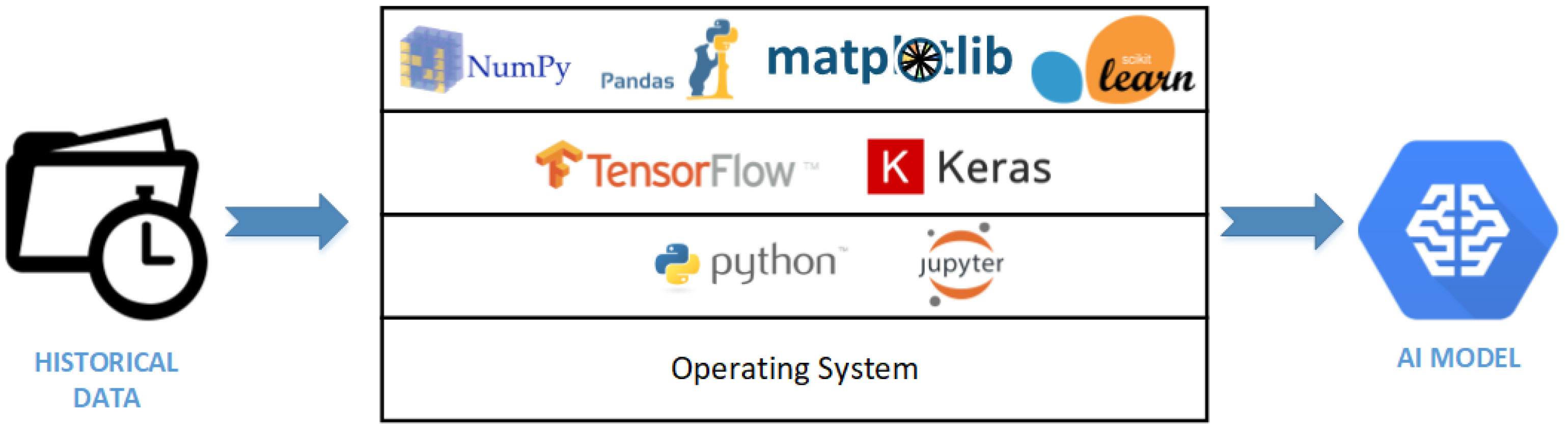
3.1. System Architecture
The system architecture is required in a specific environment to provide machine learning experiments. The datasets of fake and real news disease are trained using traditional ML and neural network models. The library used NumPy and Pandas to process data manipulation and preprocessing. Matplotlib was used to visualize real and predictive information. Scikit-learn was applied to evaluate the accuracy of the model.
Figure 1 describes the architecture of the environmental scheme used in the project.
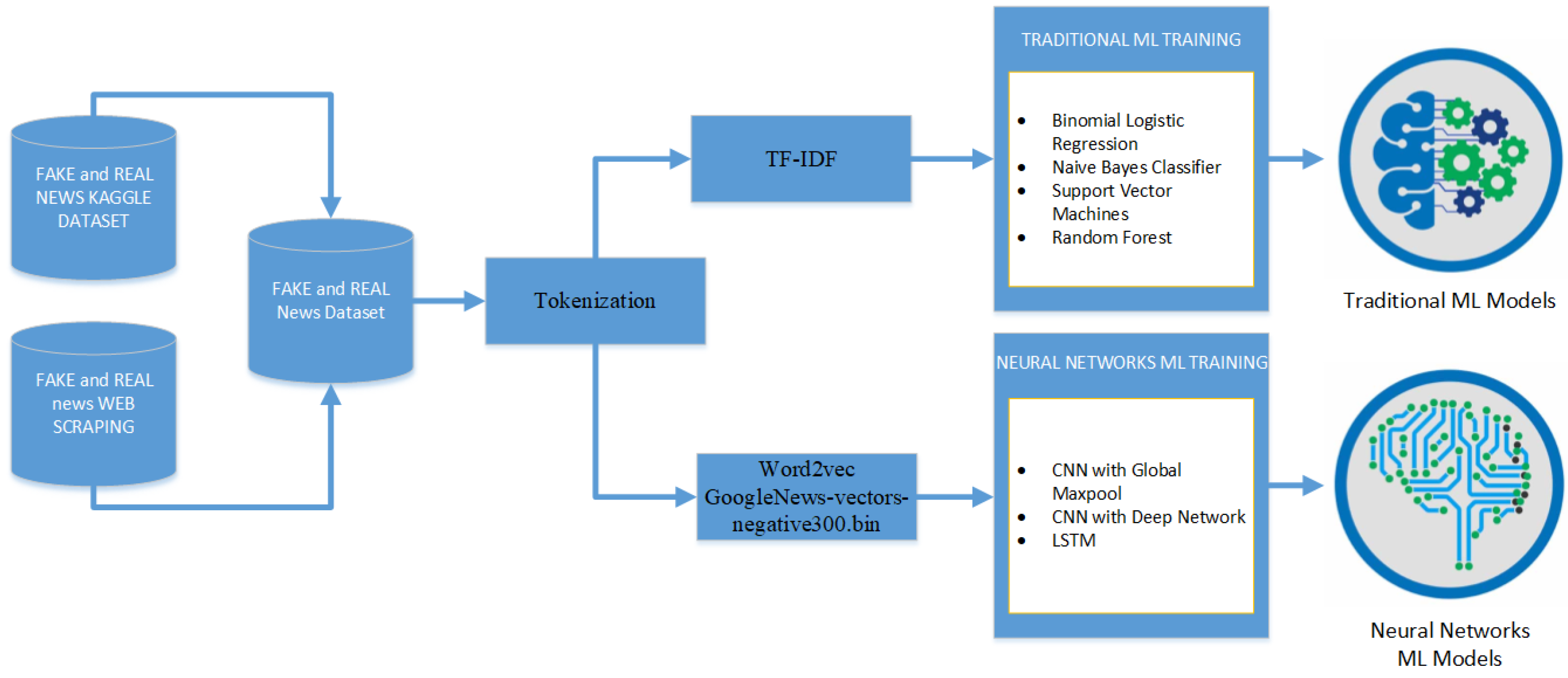
3.2. WorkFlows
Figure 2 describes the experimental procedure. First, data preprocessing was conducted using certain methods. Second, there are two kinds of training methods, using traditional ML and neural network models. Third, a comparison of ML and neural network models was presented.
3.3. Dataset Preparation
The dataset was collected from the Kaggle dataset and scraped articles. The scraped articles are from 40 link sources of news and contain 24 accountable news links and 16 unclear links. First, the dataset from Kaggle and scraped articles were integrated, and articles with only pictures or no text were removed. Additionally, because there were no clear subject categories, especially within Fake News, we removed one column of the subject. Therefore, the final column of the dataset is in four columns. Then, the dataset was split into two kinds of corpora—Fake and Real News. Next, the Tokenization process was applied to these datasets using the Natural Language Toolkit (NLTK). The detail shaped of two resources are as follows:
Kaggle, the Kaggle dataset contains fake and true news articles from 2015–2018.
FAKE SHAPE (23.481, 5)
TRUE SHAPE (21.417, 5)
Forty web-scraped news articles, from 24 accountable resources and 16 unclear resources.
FAKE SHAPE (723, 5)
TRUE SHAPE (1553, 5)
Therefore, all datasets shaped are:
FAKE (24.204, 4)
TRUE (22.970, 4)
3.4. Training Methods
There are two kinds of training methods that use traditional ML and neural network models. For the ML model, we used TF-IDF to score the words. For neural network models, we used Word2vec by Google using GoogleNews-vectors-negative300.bin. The traditional ML models implement four types of algorithms: binomial logistic regression, naive Bayes classifier, support vector machines, and random forest. The neural network models applied three kinds of algorithms: CNN with global max pool, CNN with deep networks, and LSTM. The detailed model interpretation of each algorithm is presented as follows.
3.4.1. ML Training Model
The ML models summary is listed as follows.
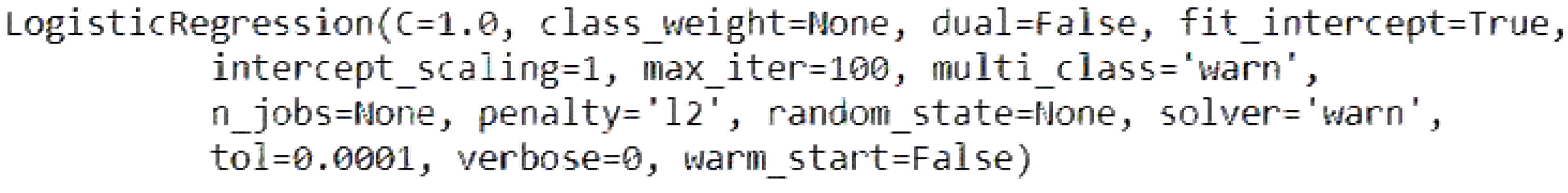
Binomial Logistic Regression
Figure 3 shows the binomial logistic regression model.
Naive Bayes Classifier
MultinomialNB (alpha=1.0, class_prior=None, fit_prior=True)
Alpha set = 1 means Additive (Laplace/Lidstone) is smoothing. Class_prior = None means prior probabilities of the classes re adjusted according to the data. Fit_prior = True means whether to learn class prior probabilities or not.
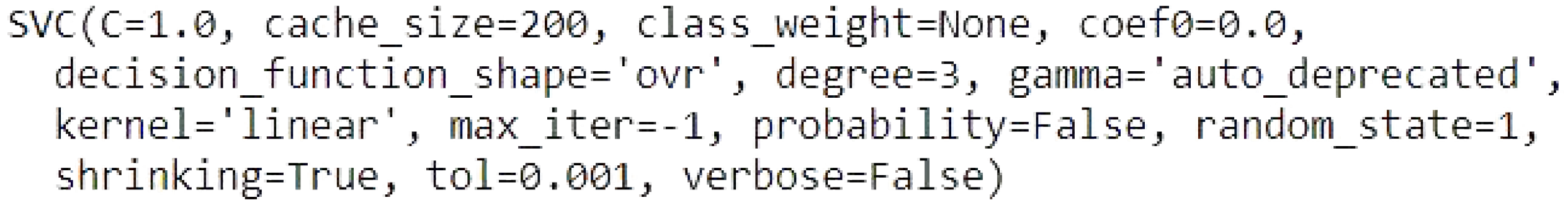
Support Vector Machines
C is the regularization parameter, the default is 1.0, cache size is the size of the kernel chache, the default is 200.
class weight is none means that all classes supposed to have weight one.
Coef0 is 0.00, this is the the default parameter for independent term in kernel function. Because we used “linear” for the kernel type, then no need to set the coef0, it is only significant in “poly” and “sigmoid”.
Decision function shape “ovr” means return a one-vs-rest (ovr) decision function of shape.
Degree 3, the degree setting is ignored by all other kernels, except “poly”.
Gamma setting is auto deprecated means that we used 1/n_features.
Kernel is “linear” means that we specify the linear kernel type to be used in the algorithm.
max_iter -1 means no limit iterations.
Probability is False means that we did not enable the probability estimation.
random_state 1 is to shuffling the data to generate the pseudo random number.
Shrinking default is True means that we use the shrinking heuristic.
tol 0.001 means the tolerance for stopping criterion, the default is 1 × 10, we set it at 0.001.
Verbose false means we disable verbose output.
Figure 4 shows the model of support vector machines.
Random Forest
: 200
Max_depth = 60 means that the maximum depth of the tree is 60. N_estimator = 200 means that the number of trees in the forest is 200.
3.4.2. Neural Networks Training Model
The neural network model summary is listed as follows.
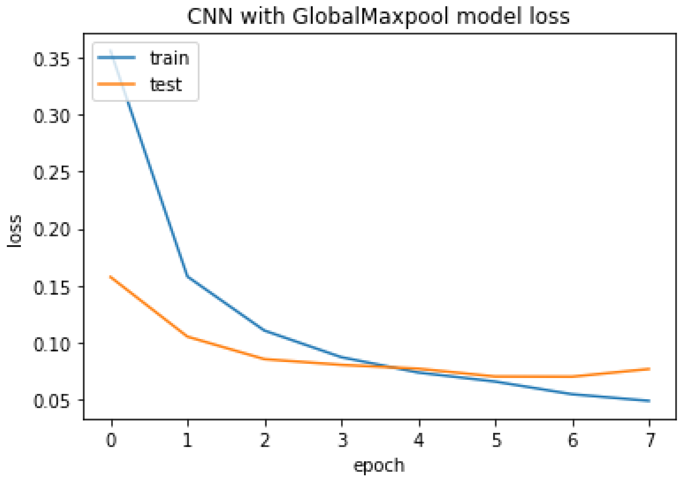
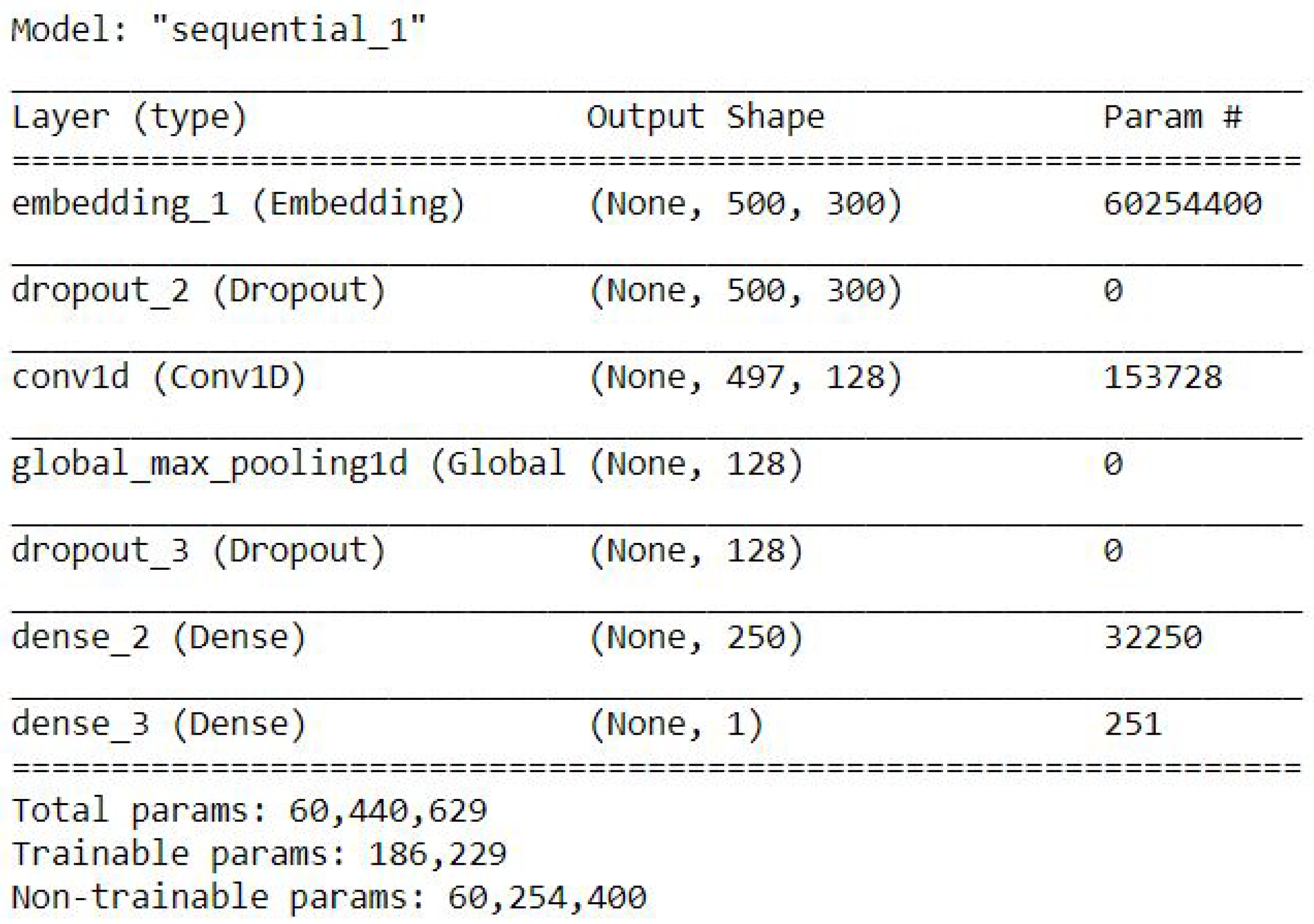
CNN with GlobalMaxpool
Figure 5 shows the CNN model with GlobalMaxpool.
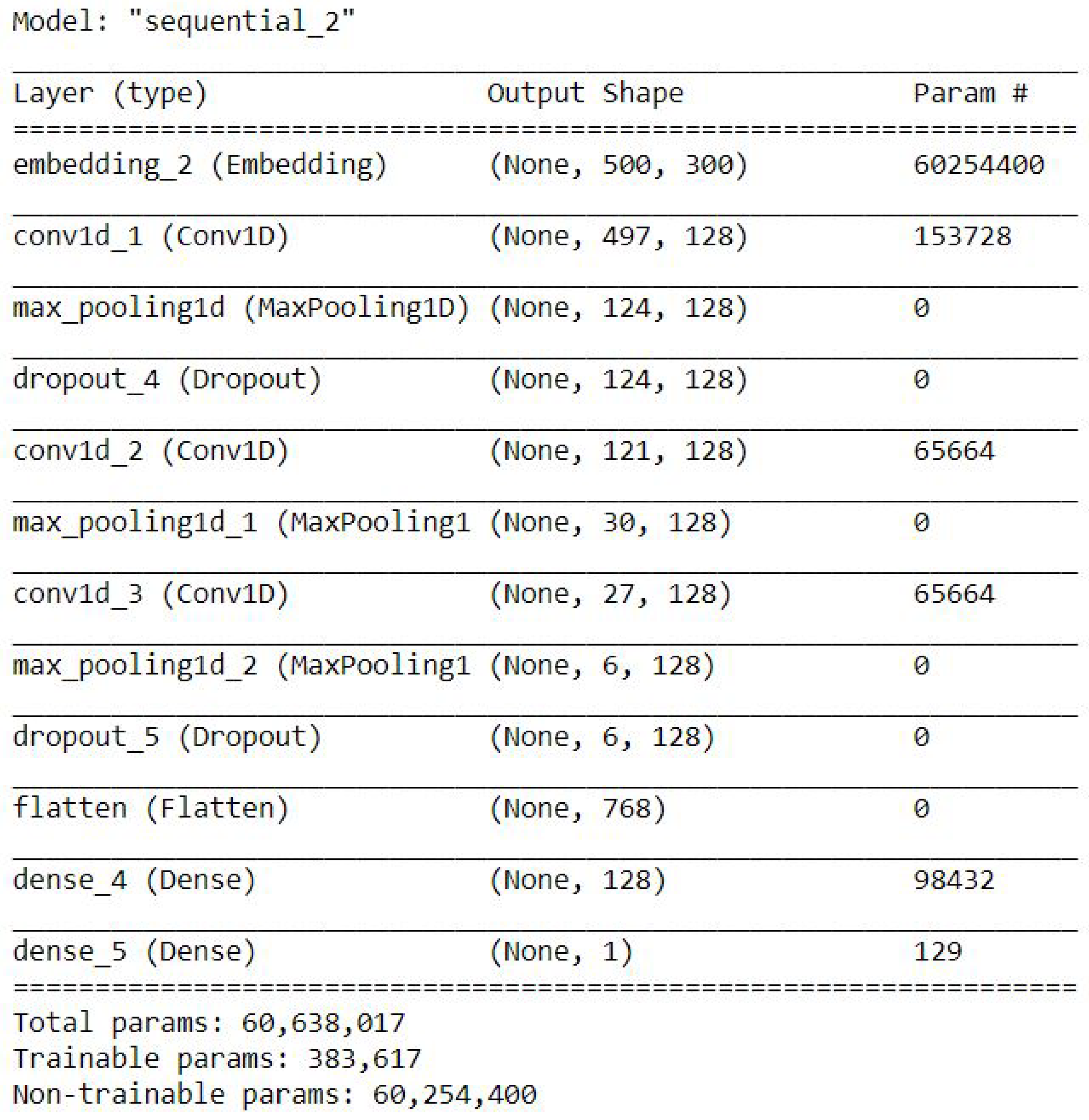
CNN with DeepNetwork
Figure 6 shows the model of CNN with DeepNetwork.
3.5. Exploratory Analysis
The exploratory data analysis describes the insight of the data.
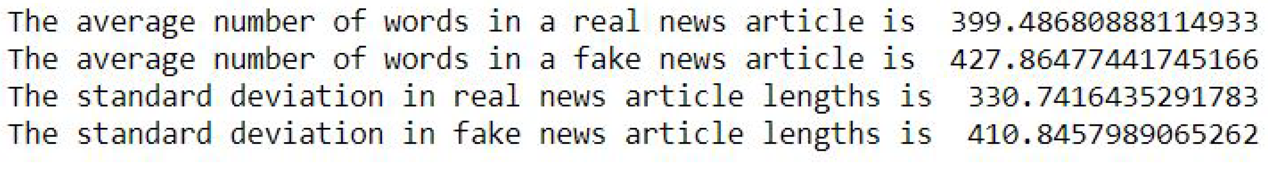
Figure 8 shows the average and standard deviation of body text.
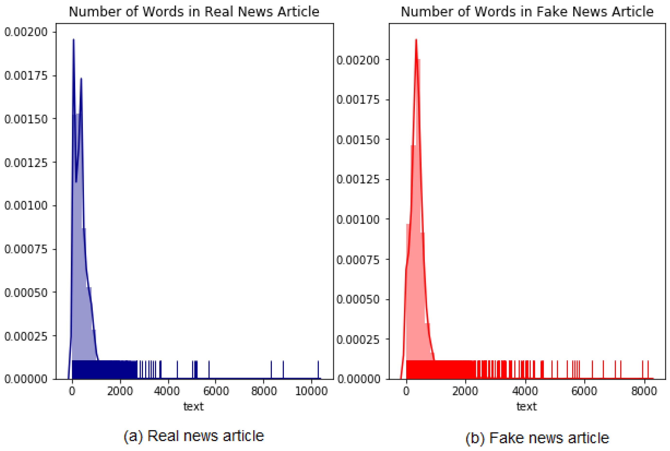
Figure 9 presents the distribution of fake and true news body text.
The average number of body text real news items is approximately 400, and the number of fake news items is 428. Therefore, the number of fake news articles is longer than the number of real news articles by approximately 28 words.
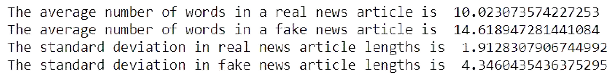
Figure 10 shows the average and standard deviation of headline text.
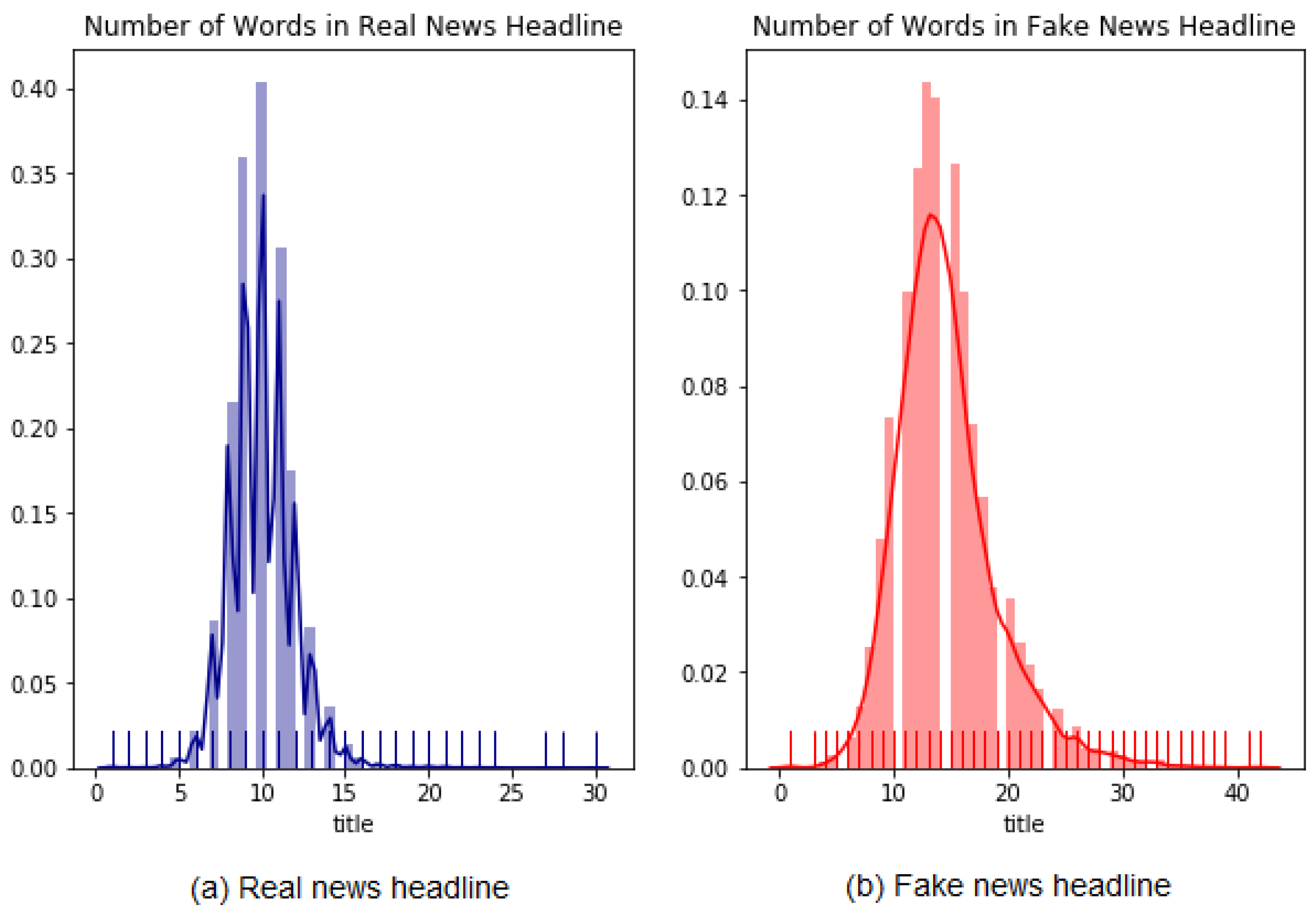
Figure 11 presents the distribution of fake and true news headline text.
The average number of titles or headlines of real news is approximately 10, and the average number of fake news is 15. Therefore, the number of fake news articles is longer than the number of real news articles by approximately five words.
4. Experimental Result
This section demonstrates the results of the training models, consisting of the RMSE, accuracy and the classification metrics of precision, recall, and F1 score.
4.1. Traditional ML Training Results
In this section, the training results are demonstrated and compared based on each model.
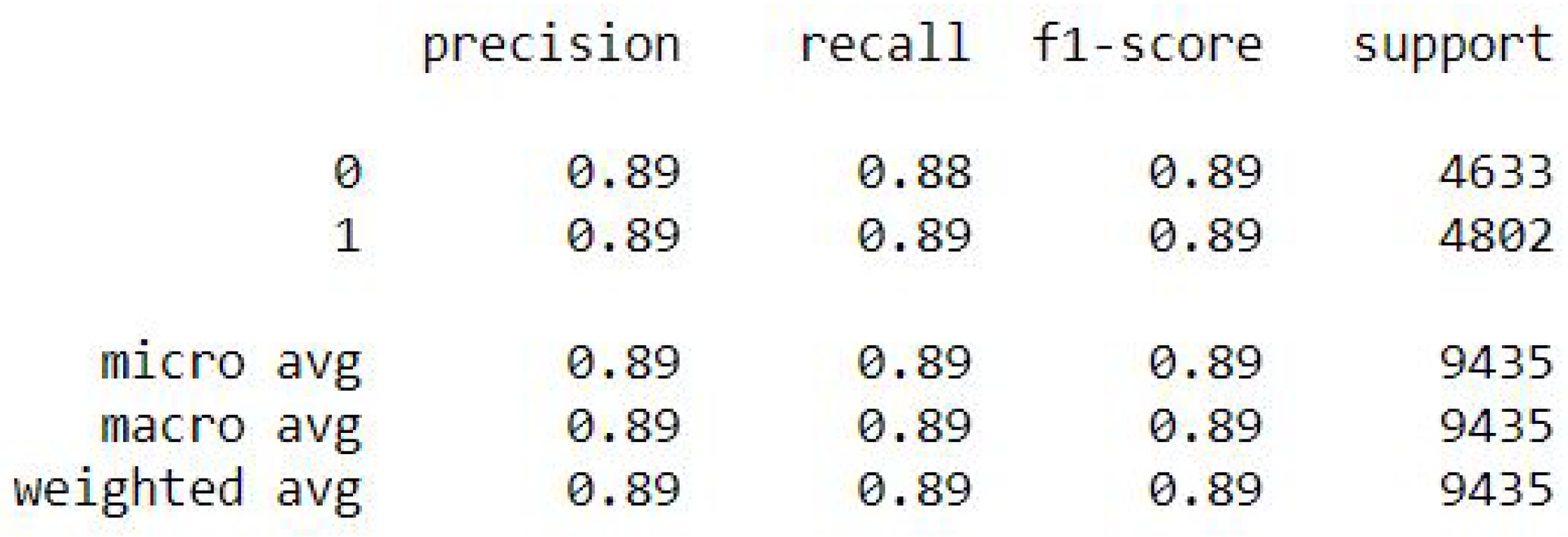
Binomial Logistic Regression
The binomial logistic regression results of the accuracy training, testing, and RMSE values are listed as follows.
Accuracy Train: 88.87357905614881
Accuracy Test: 88.88182299947006
Mean Squared Error is: 0.3334393048296787
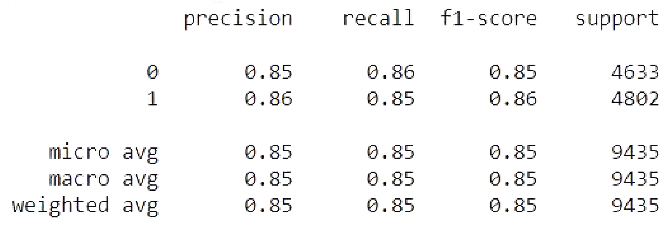
4.2. Naive Bayes
The naive Bayes results of the accuracy training, testing, and RMSE values are listed as follows.
Accuracy Train: 85.80513527120486
Accuracy Test: 85.39480657127716
Mean Squared Error is: 0.382167416569268
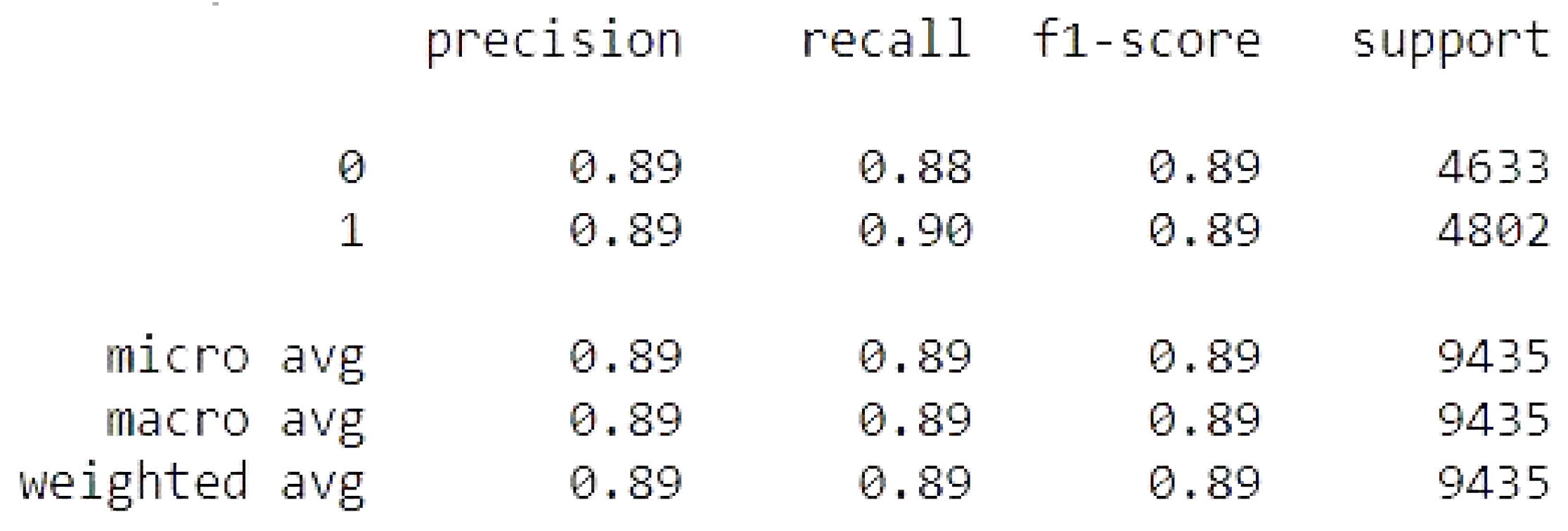
4.2.1. Support Vector Machines
The support vector machine results of the accuracy training, testing, and RMSE values are listed as follows.
Accuracy Train: 89.18360316913537
Accuracy Test: 89.01960784313725
Mean Squared Error is: 0.3313667478318056
4.2.2. Random Forest
The random forest results of the accuracy training, testing, and RMSE values are listed as follows.
Accuracy Train: 99.69792522324386
Accuracy Test: 92.87758346581876
Mean Squared Error is: 0.266878559164674
4.3. Neural Networks Training Results
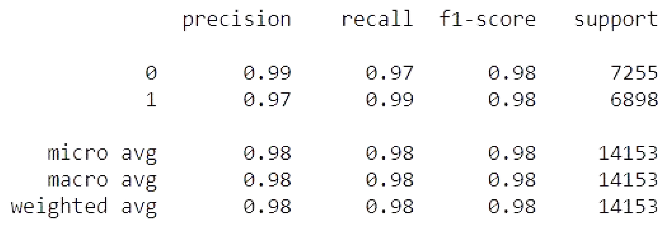
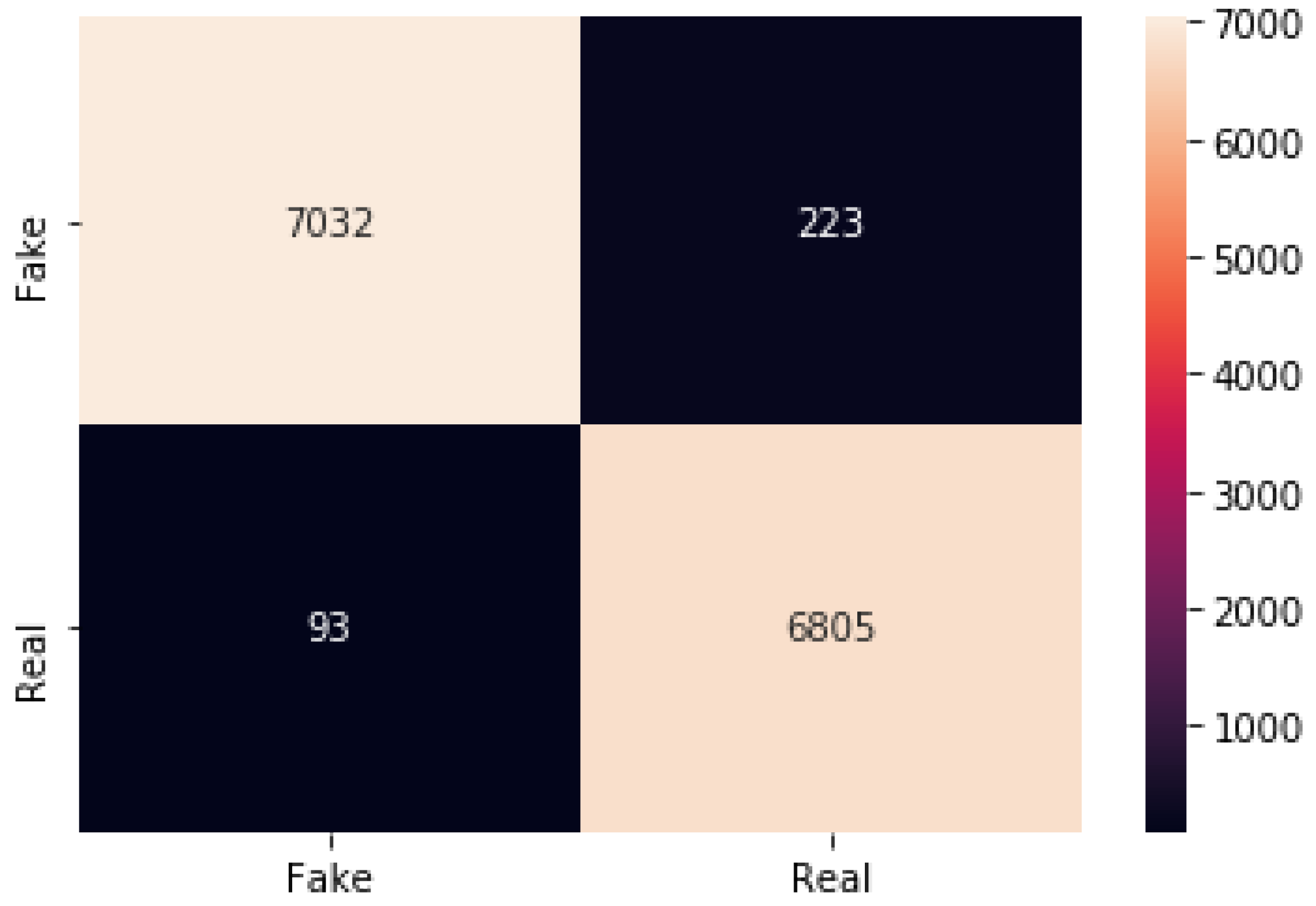
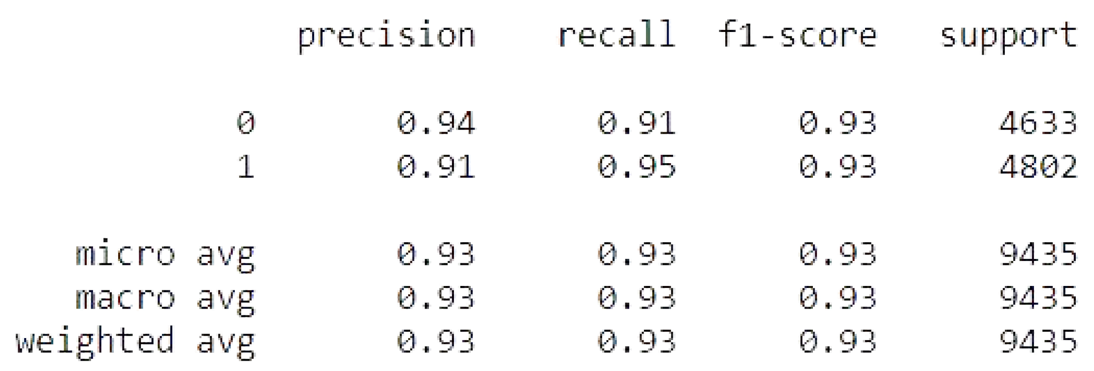
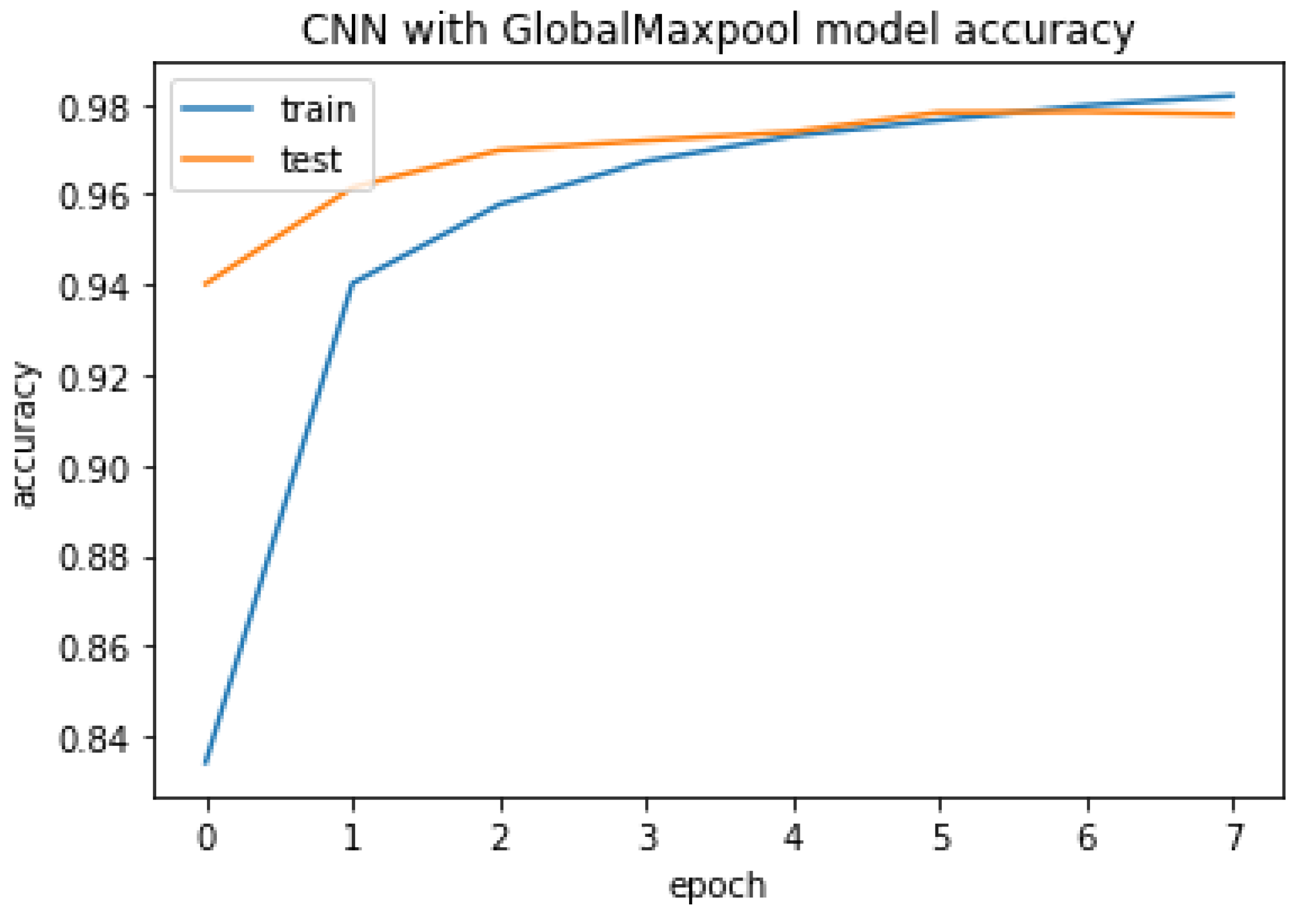
4.3.1. CNN with GlobalMaxpool
The CNN with GlobalMaxpool result of accuracy train, test, and the RMSE value are listed as follows.
Accuracy Train: 99.5457410812378
Accuracy Test: 97.76725769042969
Mean Squared Error is: 0.14942363182589052
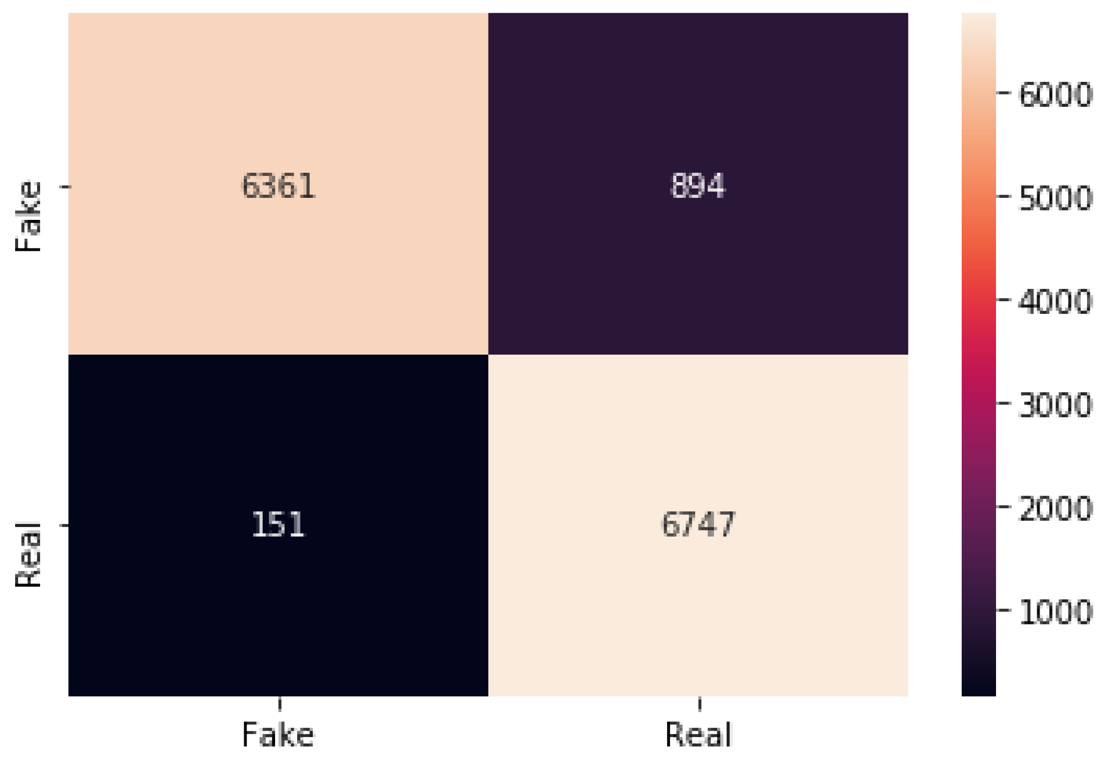
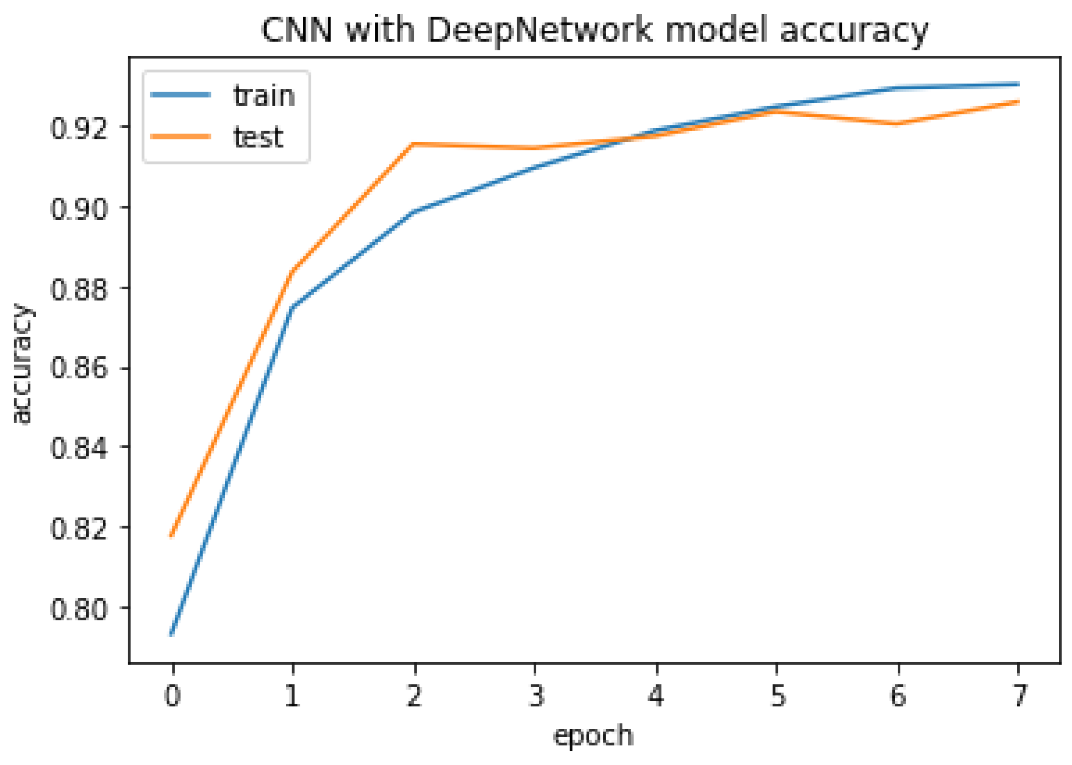
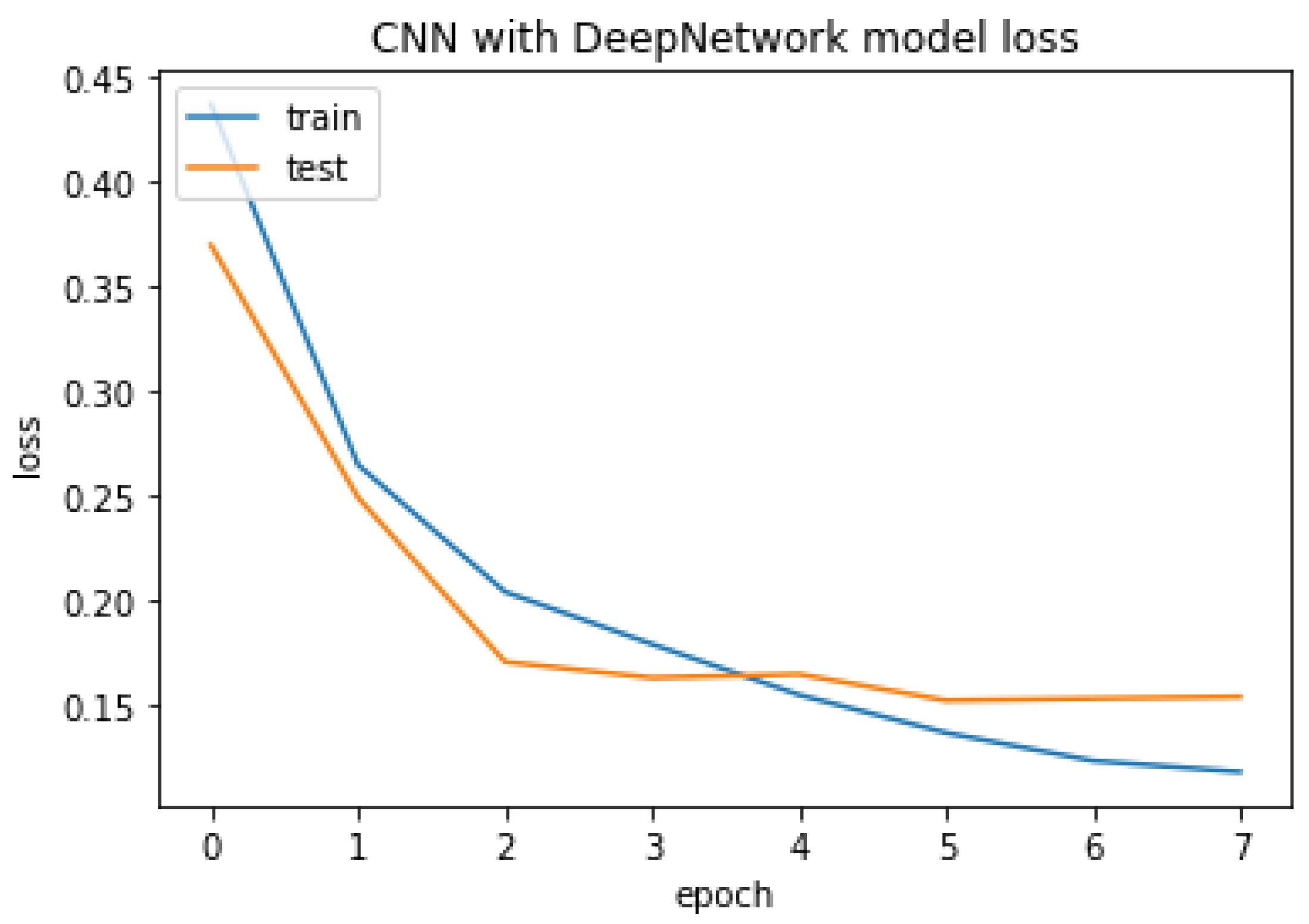
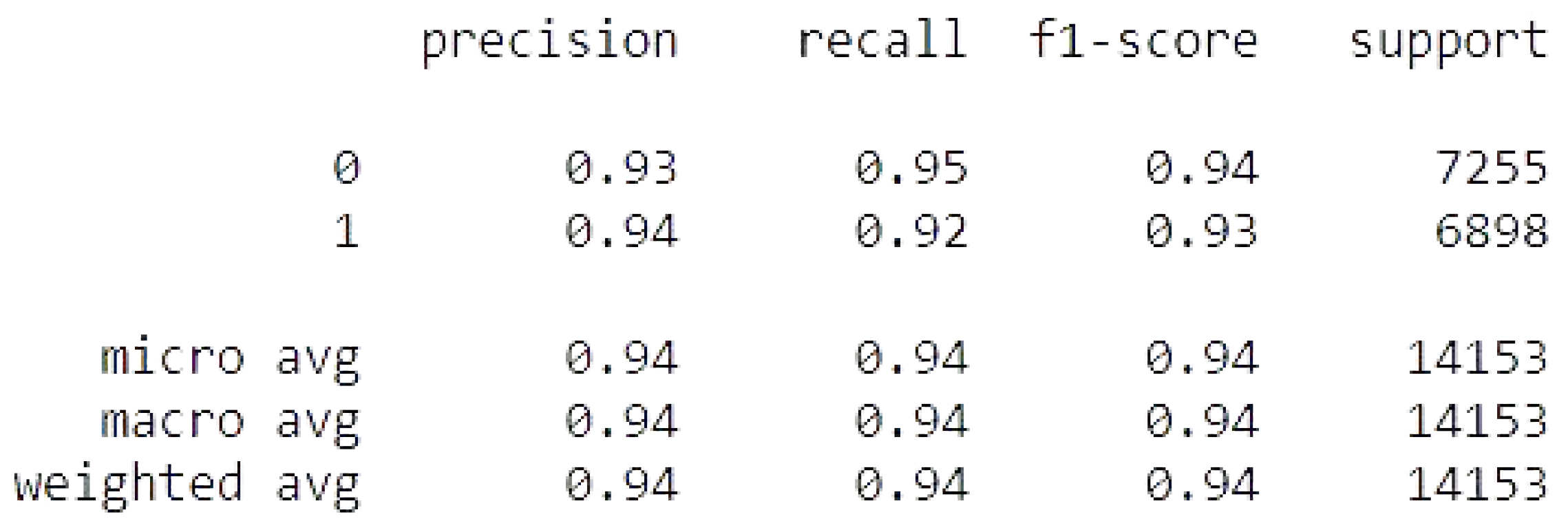
4.3.2. CNN with DeepNetwork
The CNN with DeepNetwork result of accuracy, train, test, and the RMSE value are listed as follows.
Accuracy Train: 94.30665373802185
Accuracy Test: 92.61640906333923
Mean Squared Error is: 0.2717276869293791
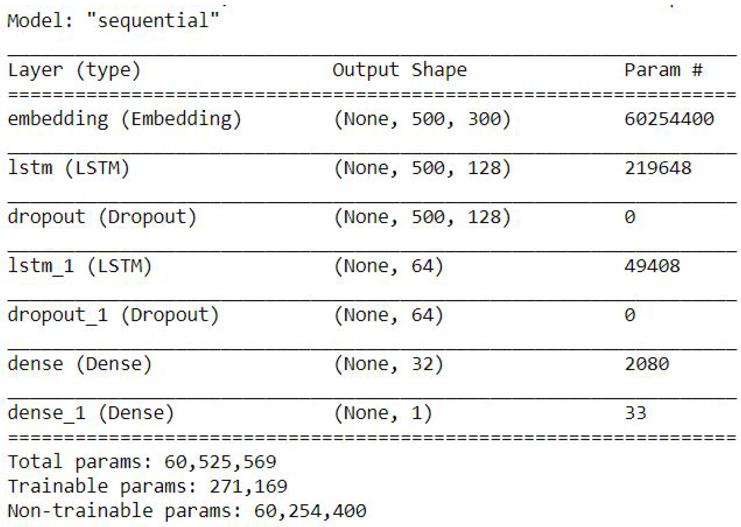
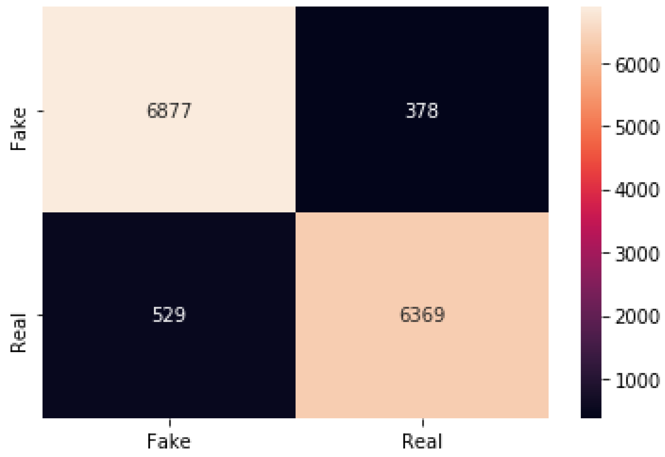
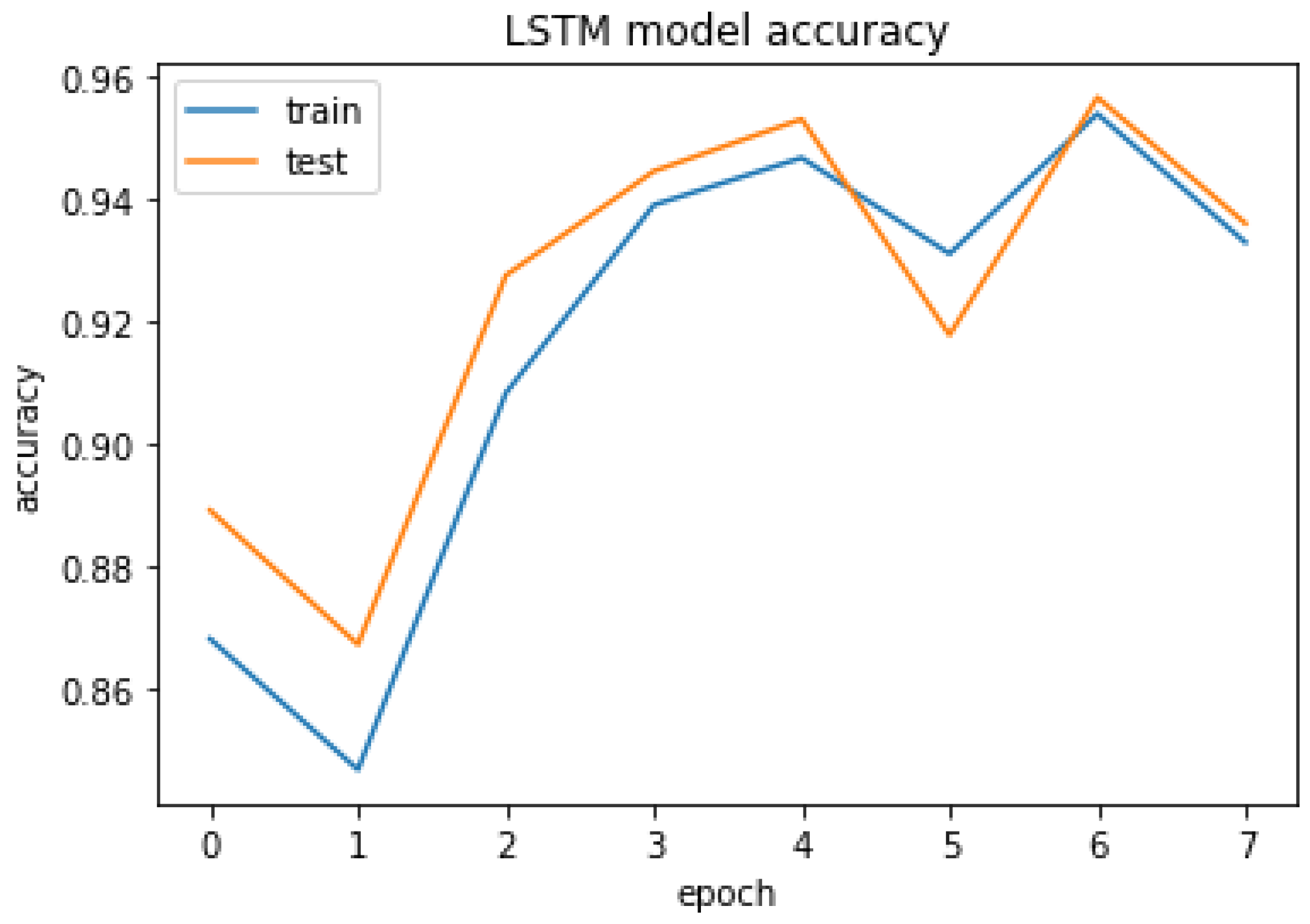
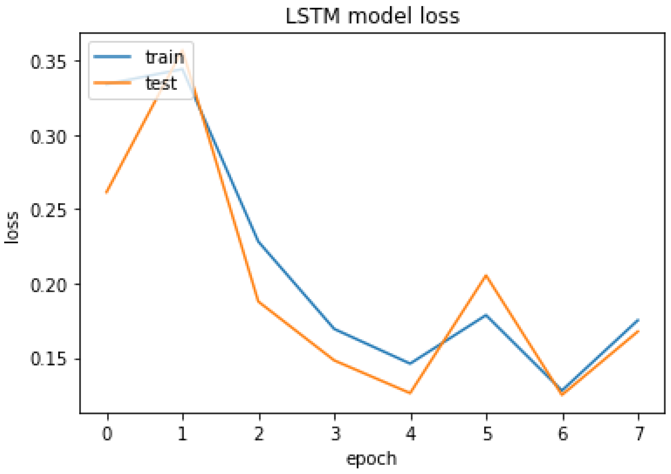
4.3.3. LSTM
The LSTM result of accuracy train, test, and the RMSE value are listed as follows.
Accuracy Train: 94.10375356674194
Accuracy Test: 93.59146356582642
Mean Squared Error is: 0.25315085014415356
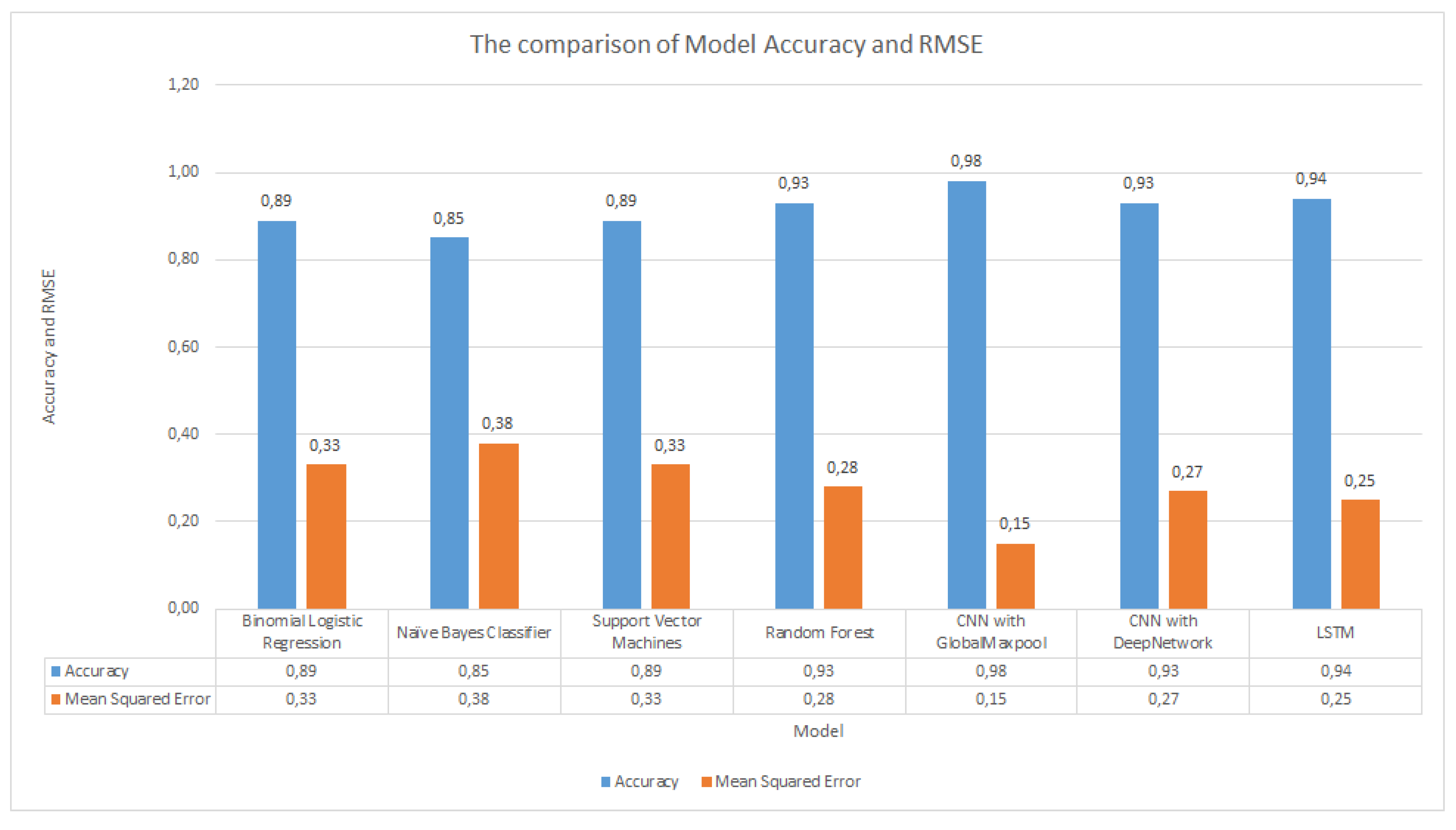
4.4. Model Comparison
Figure 32 describes the model comparison. From the graph, neural network models can be seen to outperform ML models with an accuracy of more than 90%. The RMSE values also show a lower value compared to the ML models.
4.5. Discussion
By implementing NLP methods, both ML models and neural network models have an excellent performance, with greater than 85% accuracy for all models. The neural network models outperform traditional ML models, with all neural network models reaching a greater than 90% accuracy. The best accuracy was achieved by the CNN with Global Maxpool model. There is an approximately 6% higher accuracy in neural network models than in ML models.
5. Conclusions and Future Works
This paper implemented fake news classification using machine learning, deep learning and natural language processing. NLP methods, such as Tokenize, TF-IDF and Word2vec, were applied to increase the accuracy. Traditional ML models implement four algorithms—binomial logistic regression, naive Bayes classifier, support vector machines and random forest. The neural network models utilized three algorithms—CNN with GlobalMaxpool, CNN with DeepNetwork and LSTM. The novel empirical studies from previous works were to classify tagged false news, and NLP is integrated with classical machine learning to create an AI model. On an open public dataset based on content-level attributes, we evaluate seven models to discover the best model between classical ML and neural network approaches. From the experiments, we can see that the random forest model achieves excellent accuracy compared to the other traditional ML models. CNN with GlobalMaxpool is the best neural network model among the other two models. By implementing NLP methods, all the models have a greater than 85% accuracy. All the neural network models have a greater than 90% accuracy.
In the future, various models and methods can be improved, such as using bidirectional encoder representations from transformers (BERT), applying LSTM sequences to sequences, implementing bigrams and trigrams in training traditional ML and neural network models.
Author Contributions
Conceptualization, C.-M.L. and M.-H.C.; methodology, C.-T.Y. and V.K.V.; software, E.K.; validation, V.K.V. and C.-T.Y.; formal analysis, C.-M.L. and M.-H.C.; data curation, E.K.; writing—original draft preparation, E.K.; writing—review and editing, C.-T.Y., C.-M.L. and M.-H.C. All authors have read and agreed to the published version of the manuscript.
Funding
This research was supported by the Ministry of Science and Technology, Taiwan, under grants number 110-2221-E-029-020-MY3, 110-2621-M-029-003, 110-2622-E-029-003, 110-2222-E-029-001, and 110-2222-E-029-001.
Conflicts of Interest
The authors declare that they have no known competing financial interest or personal relationships that could have appeared to influence the work reported in this paper.
References
- Johnson, W.; Bouchard, T.J., Jr. Sex differences in mental abilities: G masks the dimensions on which they lie. Intelligence 2007, 35, 23–39. [Google Scholar] [CrossRef]
- Newman, M.L.; Pennebaker, J.W.; Berry, D.S.; Richards, J.M. Lying words: Predicting deception from linguistic styles. Personal. Soc. Psychol. Bull. 2003, 29, 665–675. [Google Scholar] [CrossRef] [PubMed]
- Dey, A.; Rafi, R.Z.; Parash, S.H.; Arko, S.K.; Chakrabarty, A. Fake News Pattern Recognition using Linguistic Analysis. In Proceedings of the 2018 Joint 7th International Conference on Informatics, Electronics & Vision (ICIEV) and 2018 2nd International Conference on Imaging, Vision & Pattern Recognition (icIVPR), Kitakyushu, Japan, 25–29 June 2018; pp. 305–309. [Google Scholar] [CrossRef]
- Bondielli, A.; Marcelloni, F. A survey on fake news and rumour detection techniques. Inf. Sci. 2019, 497, 38–55. [Google Scholar] [CrossRef]
- Marquardt, D. Linguistic Indicators in the Identification of Fake News. Mediat. Stud. 2019, 3, 95–114. [Google Scholar] [CrossRef]
- Torabi Asr, F.; Taboada, M. Big Data and quality data for fake news and misinformation detection. Big Data Soc. 2019, 6, 2053951719843310. [Google Scholar] [CrossRef] [Green Version]
- Asr, F.T.; Taboada, M. The data challenge in misinformation detection: Source reputation vs. content veracity. In Proceedings of the First Workshop on Fact Extraction and Verification (FEVER), Brussels, Belgium, 1 November 2018; pp. 10–15. [Google Scholar]
- Hancock, J.T.; Curry, L.E.; Goorha, S.; Woodworth, M. On lying and being lied to: A linguistic analysis of deception in computer-mediated communication. Discourse Process. 2007, 45, 1–23. [Google Scholar] [CrossRef]
- Rashkin, H.; Choi, E.; Jang, J.Y.; Volkova, S.; Choi, Y. Truth of varying shades: Analyzing language in fake news and political fact-checking. In Proceedings of the 2017 Conference on Empirical Methods in Natural Language Processing, Copenhagen, Denmark, 7–11 September 2017; pp. 2931–2937. [Google Scholar]
- Clarke, I.; Grieve, J. Stylistic variation on the Donald Trump Twitter account: A linguistic analysis of tweets posted between 2009 and 2018. PLoS ONE 2019, 14, e0222062. [Google Scholar] [CrossRef] [PubMed] [Green Version]
- Ahmed, H.; Traore, I.; Saad, S. Detection of online fake news using n-gram analysis and machine learning techniques. In International Conference on Intelligent, Secure, and Dependable Systems in Distributed and Cloud Environments; Springer: Cham, Switzerland, 2017; pp. 127–138. [Google Scholar]
- Mikolov, T.; Sutskever, I.; Chen, K.; Corrado, G.; Dean, J. Distributed Representations of Words and Phrases and their Compositionality. In Proceedings of the 27th Annual Conference on Neural Information Processing Systems (NIPS 2013), Lake Tahoe, NV, USA, 5–8 December 2013. [Google Scholar]
- Mikolov, T.; Yih, W.t.; Zweig, G. Linguistic Regularities in Continuous Space Word Representations. In Proceedings of the 2013 Conference of the North American Chapter of the Association for Computational Linguistics: Human Language Technologies, Atlanta, GA, USA, 9–14 June 2013. [Google Scholar]
- Mikolov, T.; Chen, K.; Corrado, G.; Dean, J. Efficient Estimation of Word Representations in Vector Space. In Proceedings of the 1st International Conference on Learning Representations (ICLR, 2013), Scottsdale, AZ, USA, 2–4 May 2013. [Google Scholar]
- Wu, H.; Luk, R.; Wong, K.; Kwok, K. Interpreting TF-IDF term weights as making relevance decisions. ACM Trans. Inf. Syst. 2008, 26, 1–37. [Google Scholar] [CrossRef]
- TF-IDF. Available online: http://www.tfidf.com/ (accessed on 30 November 2019).
- TfidfVectorizer. Available online: https://scikit-learn.org/stable/modules/generated/sklearn.feature_extraction.text.TfidfVectorizer.html (accessed on 10 November 2019).
- Sparck Jones, K. A statistical interpretation of term specificity and its application in retrieval. J. Doc. 1972, 28, 11–21. [Google Scholar] [CrossRef]
- Salton, G.; Fox, E.; Wu, H. Extended Boolean information retrieval. Commun. ACM 1983, 26, 1022–1036. [Google Scholar] [CrossRef]
- Salton, G.; McGill, M.J. Introduction to Modern Information Retrieval; McGraw-Hill: New York, NY, USA, 1983. [Google Scholar]
- Salton, G.; Buckley, C. Term-weighting approaches in automatic text retrieval. Inf. Process. Manag. 1988, 24, 513–523. [Google Scholar] [CrossRef] [Green Version]
- Traylor, T.; Straub, J.; Snell, N. Classifying Fake News Articles Using Natural Language Processing to Identify In-Article Attribution as a Supervised Learning Estimator. In Proceedings of the 2019 IEEE 13th International Conference on Semantic Computing (ICSC), Newport Beach, CA, USA, 30 January–1 February 2019; pp. 445–449. [Google Scholar] [CrossRef]
- Logistic Regression. Available online: https://scikit-learn.org/stable/modules/generated/sklearn.linear_model.LogisticRegression.html (accessed on 10 March 2020).
- Granik, M.; Mesyura, V. Fake news detection using naive Bayes classifier. In Proceedings of the 2017 IEEE First Ukraine Conference on Electrical and Computer Engineering (UKRCON), Kyiv, Ukraine, 29 May–2 June 2017; pp. 900–903. [Google Scholar]
- Naive Bayes. Available online: https://scikit-learn.org/stable/modules/generated/sklearn.naive_bayes.MultinomialNB.html (accessed on 15 January 2020).
- Support Vector Classification. Available online: https://scikit-learn.org/stable/modules/generated/sklearn.svm.SVC.html,sklearn.svm.SVC (accessed on 18 February 2020).
- Random Forest. Available online: https://scikit-learn.org/stable/modules/generated/sklearn.ensemble.RandomForestClassifier.html (accessed on 12 February 2020).
- Hochreiter, S.; Schmidhuber, J. LSTM can solve hard long time lag problems. In Advances in Neural Information Processing Systems; The MIT Press: Cambridge, MA, USA, 1997; pp. 473–479. [Google Scholar]
- Ahmed, H.; Traore, I.; Saad, S. Detecting opinion spams and fake news using text classification. Secur. Priv. 2018, 1, e9. [Google Scholar] [CrossRef] [Green Version]
- Reis, J.C.; Correia, A.; Murai, F.; Veloso, A.; Benevenuto, F. Supervised learning for fake news detection. IEEE Intell. Syst. 2019, 34, 76–81. [Google Scholar] [CrossRef]
- Asghar, M.Z.; Habib, A.; Habib, A.; Khan, A.; Ali, R.; Khattak, A. Exploring deep neural networks for rumor detection. J. Ambient. Intell. Humaniz. Comput. 2019, 12, 4315–4333. [Google Scholar] [CrossRef]
- Goldani, M.H.; Safabakhsh, R.; Momtazi, S. Convolutional neural network with margin loss for fake news detection. Inf. Process. Manag. 2021, 58, 102418. [Google Scholar] [CrossRef]
- Hakak, S.; Alazab, M.; Khan, S.; Gadekallu, T.R.; Maddikunta, P.K.R.; Khan, W.Z. An ensemble machine learning approach through effective feature extraction to classify fake news. Future Gener. Comput. Syst. 2021, 117, 47–58. [Google Scholar] [CrossRef]
- Umer, M.; Imtiaz, Z.; Ullah, S.; Mehmood, A.; Choi, G.S.; On, B.W. Fake news stance detection using deep learning architecture (cnn-lstm). IEEE Access 2020, 8, 156695–156706. [Google Scholar] [CrossRef]
- Nasir, J.A.; Khan, O.S.; Varlamis, I. Fake news detection: A hybrid CNN-RNN based deep learning approach. Int. J. Inf. Manag. Data Insights 2021, 1, 100007. [Google Scholar] [CrossRef]
Figure 1.
System Architecture.
Figure 1.
System Architecture.
Figure 2.
Workflows Diagram.
Figure 2.
Workflows Diagram.
Figure 3.
Binomial Logistic Regression Model.
Figure 3.
Binomial Logistic Regression Model.
Figure 4.
Support Vector Machines Model.
Figure 4.
Support Vector Machines Model.
Figure 5.
CNN with GlobalMaxpool Model.
Figure 5.
CNN with GlobalMaxpool Model.
Figure 6.
CNN with DeepNetwork Model.
Figure 6.
CNN with DeepNetwork Model.
Figure 8.
The average and standard deviation of body text.
Figure 8.
The average and standard deviation of body text.
Figure 9.
The distribution of Real and Fake news body text.
Figure 9.
The distribution of Real and Fake news body text.
Figure 10.
The average and standard deviation of headlines text.
Figure 10.
The average and standard deviation of headlines text.
Figure 11.
The distribution of Real and Fake news headlines text.
Figure 11.
The distribution of Real and Fake news headlines text.
Figure 12.
Binomial Logistic Regression metrics.
Figure 12.
Binomial Logistic Regression metrics.
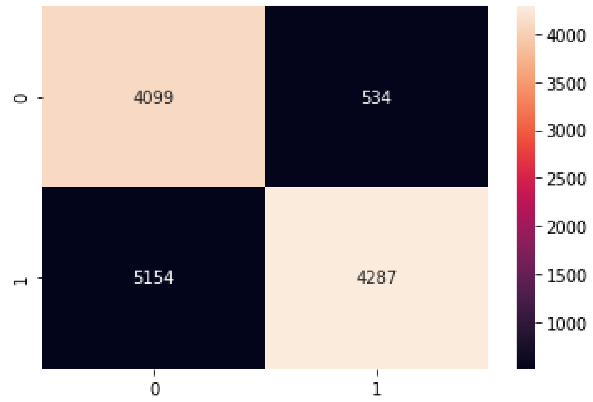
Figure 13.
Binomial Logistic Regression confusion matrix.
Figure 13.
Binomial Logistic Regression confusion matrix.
Figure 14.
Naive Bayes metrics.
Figure 14.
Naive Bayes metrics.
Figure 15.
Naive Bayes confusion matrix.
Figure 15.
Naive Bayes confusion matrix.
Figure 16.
Support Vector Machines metrics.
Figure 16.
Support Vector Machines metrics.
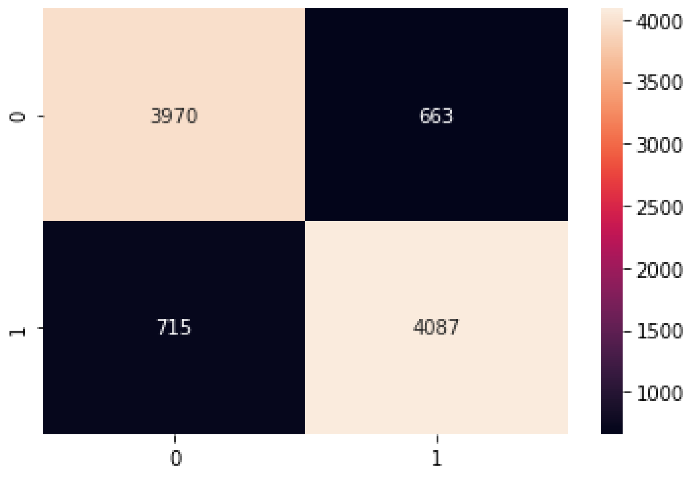
Figure 17.
Support Vector Machines confusion matrix.
Figure 17.
Support Vector Machines confusion matrix.
Figure 18.
Random Forest metrics.
Figure 18.
Random Forest metrics.
Figure 19.
Random Forest confusion matrix.
Figure 19.
Random Forest confusion matrix.
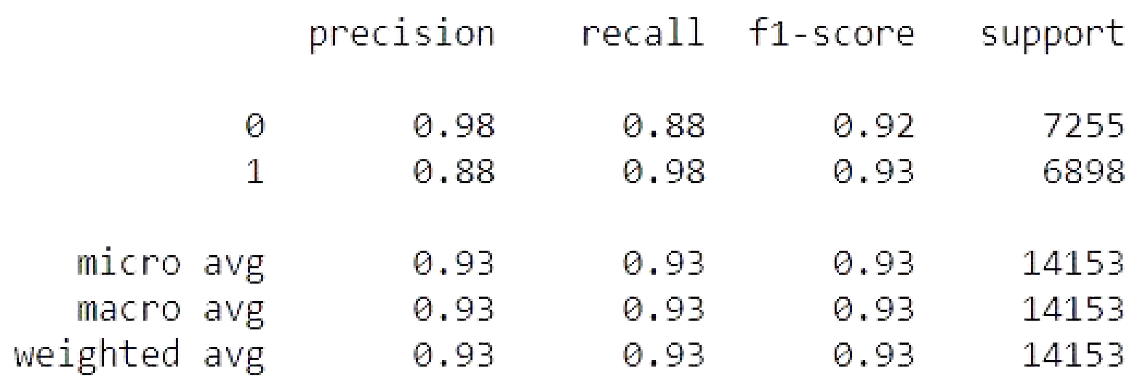
Figure 20.
CNN with GlobalMaxpool metrics.
Figure 20.
CNN with GlobalMaxpool metrics.
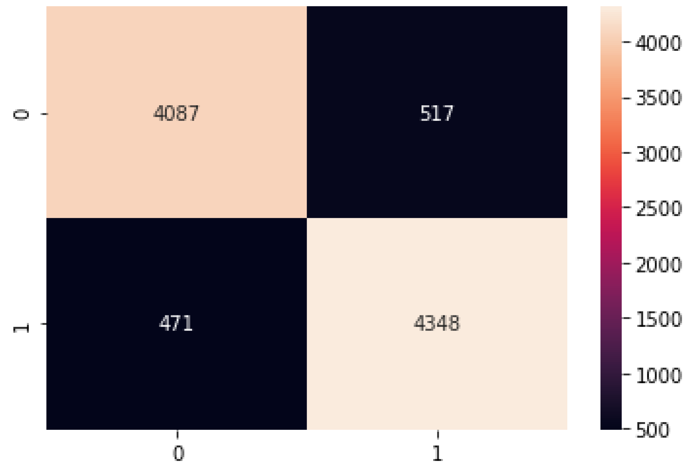
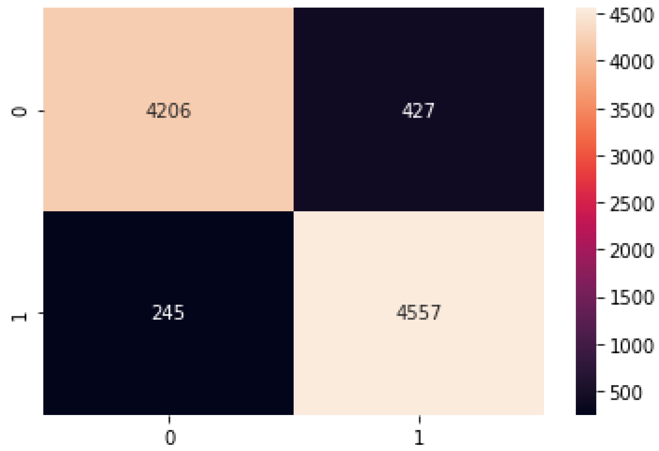
Figure 21.
CNN with GlobalMaxpool confusion matrix.
Figure 21.
CNN with GlobalMaxpool confusion matrix.
Figure 22.
CNN with GlobalMaxpool model accuracy.
Figure 22.
CNN with GlobalMaxpool model accuracy.
Figure 23.
CNN with GlobalMaxpool model loss.
Figure 23.
CNN with GlobalMaxpool model loss.
Figure 24.
CNN with DeepNetwork metrics.
Figure 24.
CNN with DeepNetwork metrics.
Figure 25.
CNN with DeepNetwork confusion matrix.
Figure 25.
CNN with DeepNetwork confusion matrix.
Figure 26.
CNN with DeepNetwork model accuracy.
Figure 26.
CNN with DeepNetwork model accuracy.
Figure 27.
CNN with DeepNetwork model loss.
Figure 27.
CNN with DeepNetwork model loss.
Figure 29.
LSTM confusion matrix.
Figure 29.
LSTM confusion matrix.
Figure 30.
LSTM model accuracy.
Figure 30.
LSTM model accuracy.
Figure 31.
LSTM model loss.
Figure 31.
LSTM model loss.
Figure 32.
The comparison of model Accuracy and RMSE.
Figure 32.
The comparison of model Accuracy and RMSE.
| Publisher’s Note: MDPI stays neutral with regard to jurisdictional claims in published maps and institutional affiliations. |
© 2022 by the authors. Licensee MDPI, Basel, Switzerland. This article is an open access article distributed under the terms and conditions of the Creative Commons Attribution (CC BY) license (https://creativecommons.org/licenses/by/4.0/).


 ,
, 
