High-Resolution Phosphorescence Lifetime Imaging (PLIM) of Bones

Abstract

For the first time, the time-resolved two-photon excited autophosphorescence of non-labeled biological specimens was investigated by phosphoresce lifetime imaging with microscopic spatial resolution. A modified multiphoton tomograph was employed to record both photoluminescence contributions, autofluorescence and autophosphorescence, simultaneously, induced by two-photon excitation using an 80 MHz near infrared femtosecond-pulse-laser scanning beam, an acousto-optic modulator, and a time-correlated single-photon counting module for lifetime measurements from the picosecond to the microsecond range. In particular, the two-photon-excited luminescence of thermally altered bones was imaged. A strong dependence of the phosphorescence intensity on exposure temperature, with a maximum emission for an exposure temperature of approximately 600 °C was observed. Furthermore, the phosphorescence lifetime data indicated a bi-exponential signal decay with both a faster few µs decay time in the range of 3–10 µs and a slower one in the range of 30–60 µs. The recording of fluorescence and phosphorescence allowed deriving the relative signal proportion as an unbiased measure of the temperature dependence. The measurements on thermally altered bones are of particular interest for application to forensic and archeological investigations.

1. Introduction

Luminescence examinations of bone samples can provide valuable forensic information and archeological insight into the environmental conditions a find was exposed to. Recently, the photoluminescence emission, in particular, of heated bones has been found to be affected by the exposure temperature [1,2,3]. Photoluminescence consists of both quickly decaying fluorescence with lifetimes in the picosecond and nanosecond range and longer prevailing phosphoresce with lifetimes in the microsecond to minute range. In particular, the study of the phosphorescence could aid in the search of human skeletal remains or indicate the maximum temperature a bone has been exposed to, for example during a previous fire as has been proposed by Krap et al. [1,3]. In Ref. [3], the authors have quantified the phosphorescence intensity by visual inspection and observer assessment through a scoring index scheme. The authors found the visibly observable phosphorescence intensity to depend strongly on the maximum exposure temperature, with the highest emissions observed in the range from 450 °C to 800 °C, and to a much lesser degree to depend on exposure duration. Photoluminescence of bones has been observed before [4] and originally assumed to stem mainly from organic substances like collagen, which is known to fluoresce but does not phosphoresce, and to a lower degree to bone minerals (e.g., apatite). Recent studies have suggested, however, that inorganic material of the bone generates the temperature-dependent phosphorescence, in particular, the main inorganic component hydroxyapatite [1,5]. The detailed microscopic origins and the components contributing to phosphorescence in particular in the range of 700 °C to 800 °C are not fully understood and for lower exposure temperatures even contradicting findings on the role of organic and inorganic components have been reported [3]. So far mainly spectroscopy methods, which have been based on continuous excitation with UV or blue light, have been used to investigate the bone photoluminescence. Krap et al. suggested to distinguish between “short-decay” and “long-decay” phosphorescence with the short-decay phosphoresce being the part which is “visibly not observable” but has a longer decay time than fluorescence [3].

In life sciences, phosphorescence lifetime microscopy (PLIM) has been used so far mainly for studies in cell biology to investigate the oxygen consumption of single cells during the cell metabolism by recording phosphorescence from exogenous markers (metal complexes) [6,7]. The marker phosphorescence emission can be affected by the system under study, e.g., a cell, and thereby indirectly indicates the sample condition. The technique can be combined with fluorescence lifetime imaging (FLIM) [8,9,10]. The novelty of this study lies in the measurement of autophosphorescence, an intrinsic sample property, in contrast to measuring phosphorescence from an externally added marker. Autophosphorescence is usually very weak or absent in biological samples but can be considered as a “direct signal” from the specimen. To the best of our knowledge the autophosphorescence of biological specimens has not been studied (i) with high-resolution microscopy/tomography, (ii) with two-photon excitation, and (iii) with precise time resolution. In this paper, we have used high-resolution femtosecond laser scanning imaging in combination with time-correlated single-photon counting (TCSPC, [9]) to investigate the spatial and temporal distributions of the two-photon excited autophosphorescence and autofluorescence emission from bones without any additional labeling with phosphorescent markers. The measurements provided the microscopic distribution of autophosphorescent substances in heated bone samples within a temporal measurement range of tens of microseconds as well as the simultaneous measurement of fast decaying fluorescence in the picosecond/nanosecond range. By evaluating the fluorescence-to-phosphorescence intensity ratio, the temperature effect on the bone photoluminescence could be unbiasedly derived and quantified without the need for a scoring index by observers.

2. Materials and Methods

2.1. Imaging System

The functionality of a commercial multiphoton tomograph (MPTflex-CARS [10,11,12,13]), JenLab, Germany) was extended by including phosphorescence lifetime imaging capability (Figure 1a). The tomograph enables, in its original configuration, in vivo and ex vivo multimodal multiphoton microscopy including fluorescence, second harmonic generation (SHG), and coherent anti-Stokes Raman scattering microscopy (CARS) as well as fluorescence lifetime imaging (FLIM) [9,10]. The mobile system contains a tunable 80 MHz femtosecond laser (MaiTai HP-JL, Newport Spectra Physics), that generates ultrashort pulses for two-photon excitation. The tomograph is outfitted with a TCSPC module (SPC-150, Becker& Hickl, Germany) in combination with a photo multiplier module (PMT) with a fast response time [9]. Imaging is achieved with a laser scanning setup, which is integrated inside a flexibly positionable scan-detector unit, i.e., by scanning-focused laser pulses pixelwise across a sample region through deflection by a pair of galvo-scanner mirrors [14,15]. The laser power that reaches the sample can be regulated with an acoustic optical modulator (AOM, AA opto-electronic, France). All signals are collected in reflection geometry and can be detected in up to four spectral channels equipped with PMTs [12]. For the imaging of the bone samples, the flexible measuring head was set vertically such that the laser light was emitted upwards and an inverse microscope setup was realized. The samples were put on a cover slip and imaged from below with a high-NA objective (1.35NA-40x Uapo; Olympus) which focused the incoming laser pulses and collected signals in reflection geometry. After the signal-laser light separation with a beamsplitter (LP 705, Semrock, Rochester, NY, USA) and the blocking of residual laser light by a short pass filter (SP680, Semrock, Rochester, NY, USA), all signals were detected in a one spectral channel within the range of 350 to 680 nm by a PMT (R9880-20, Hamamatsu, Japan). For better index of refraction matching, the samples were placed in a drop of water. All measurements were performed at room temperature.

The functionality to record in addition phosphorescence was achieved by adding a delay generator card (DDG-210, Becker & Hickel, Berlin, Germany) which, in combination with the AOM, allowed to limit the laser irradiation duration for each pixel to a fraction of the pixel dwell time [9]. In contrast to fluorescence, which results from fast singlet-to-ground-state relaxation, (triplet) phosphorescence is based on the decay of a long-lived triplet state with lifetimes in the µs range. The different lifetime ranges of fluorescence and phosphorescence as well as the ability to control both the pixel dwell and irradiation times are critical for the separate detection of both signals. In order to record the phosphoresce pixelwise, the duration of the laser illumination needs to be shorter than the pixel dwell time. For the measurements described here, the pixel dwell time was set to 110 µs. During that time the laser was unblocked (“laser on”) from 1–56 µs and blocked (“laser off”) afterwards (56 µs–110 µs), hence, the “laser-on” and “laser-off” durations were 55 µs and 54 µs each. During these time durations, signals from the sample were recorded in 1024-time channels with time steps of 100 ns. The “laser-on signal” is dominated by the fluorescence with neglectable phosphoresce contribution. During the “laser-off time”, the fluorescence quickly fades such that only the phosphoresce signal remains which can then be exclusively (background free) detected. Figure 1b illustrates this temporal dependence of the recorded signals. For the measurements reported throughout the paper, the following laser settings were chosen: the laser wavelength was set to 800 nm which corresponded to a wavelength of 400 nm for one-photon excitation. The mean laser in situ power was set to 24 mW which resulted in a mean power of 14 mW for the effectively reduced duty-cycle excitation during the imaging. Scanning with 512 × 512 pixels with approximately 30 s per frame was realized by the galvo scanners. Ten frames were subsequently recorded and the signals summed to increase the signal-to-noise ratio. In the phosphorescence lifetime images, the image pixels were reduced to 256 × 256 image pixels by binning. The decay times were analyzed with the software SPCImage (Becker & Hickl, Berlin, Germany) by performing two-exponential decay fitting. For the “global analysis”, the photon counts for all image pixels were summed up.

2.2. Samples

Chicken wings were purchased from a local supermarket. The wings were baked in a kitchen oven up to 170 °C and afterwards manually defleshed. Transverse sections with lengths of 1 to 1.5 cm were cut from the lower wing (radius and ulna bones). The bones sections were stored at room temperature and heated in a muffle furnace (L 15 Nabertherm, Germany) the next day. For the heating process, all bone samples were placed into the furnace chamber which was heated up at a rate of 100 °C/30 min. At approximately 400 °C, 500 °C, 600 °C, 700 °C, 800 °C, and 900 °C, the heating-up was interrupted and the temperature kept constant for 15 min. Two to three bone sections were then removed from the furnace and the heating resumed with the remaining samples. In this way, all bone samples were exposed to the different maximum temperatures for 15 min.

3. Results and Discussion

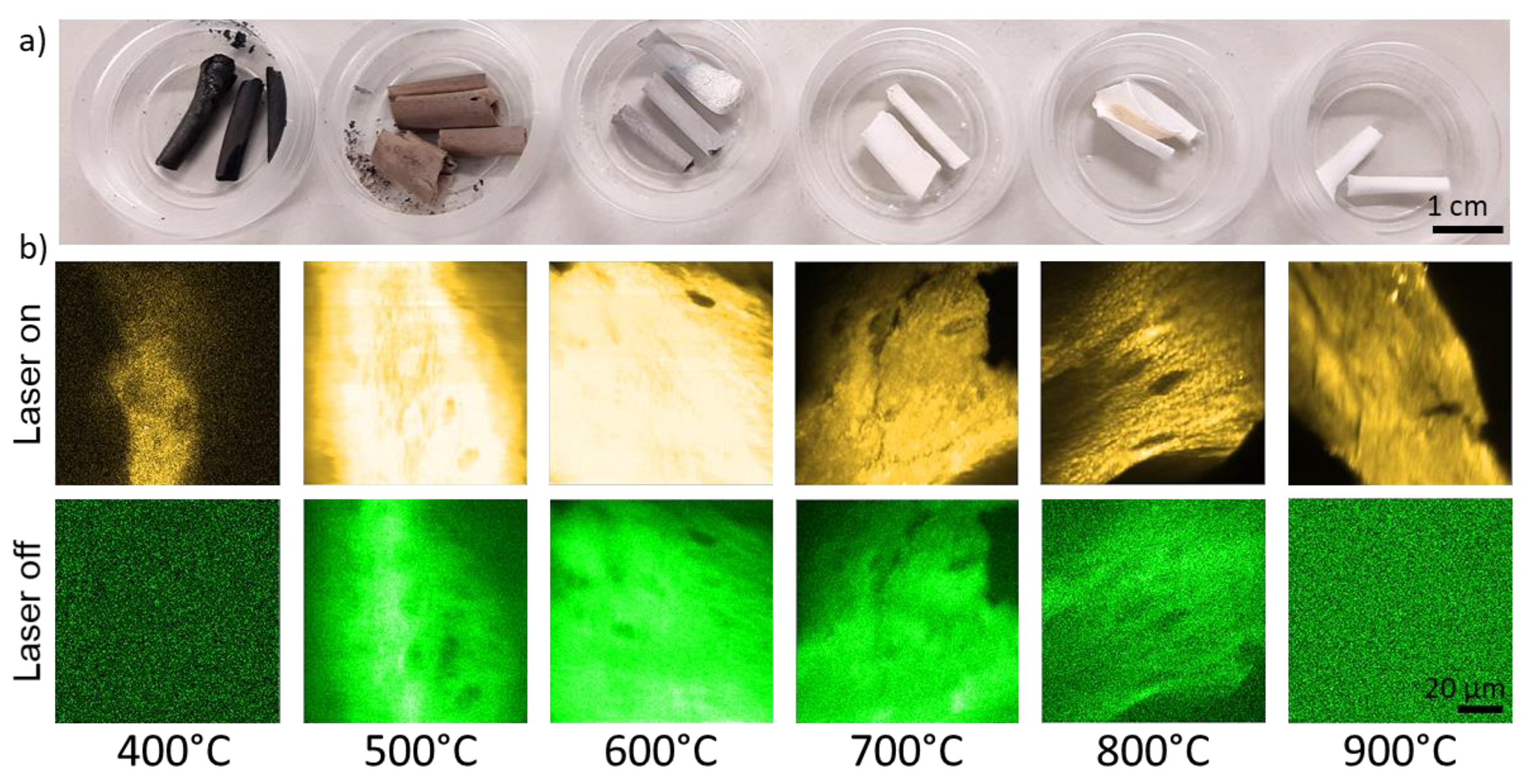
A photographic image of the bones samples after the heating which feature typical heat-induced color changes [16] is shown in Figure 2a. The color ranges from black (400 °C) to brown and grey and completely white (900 °C).

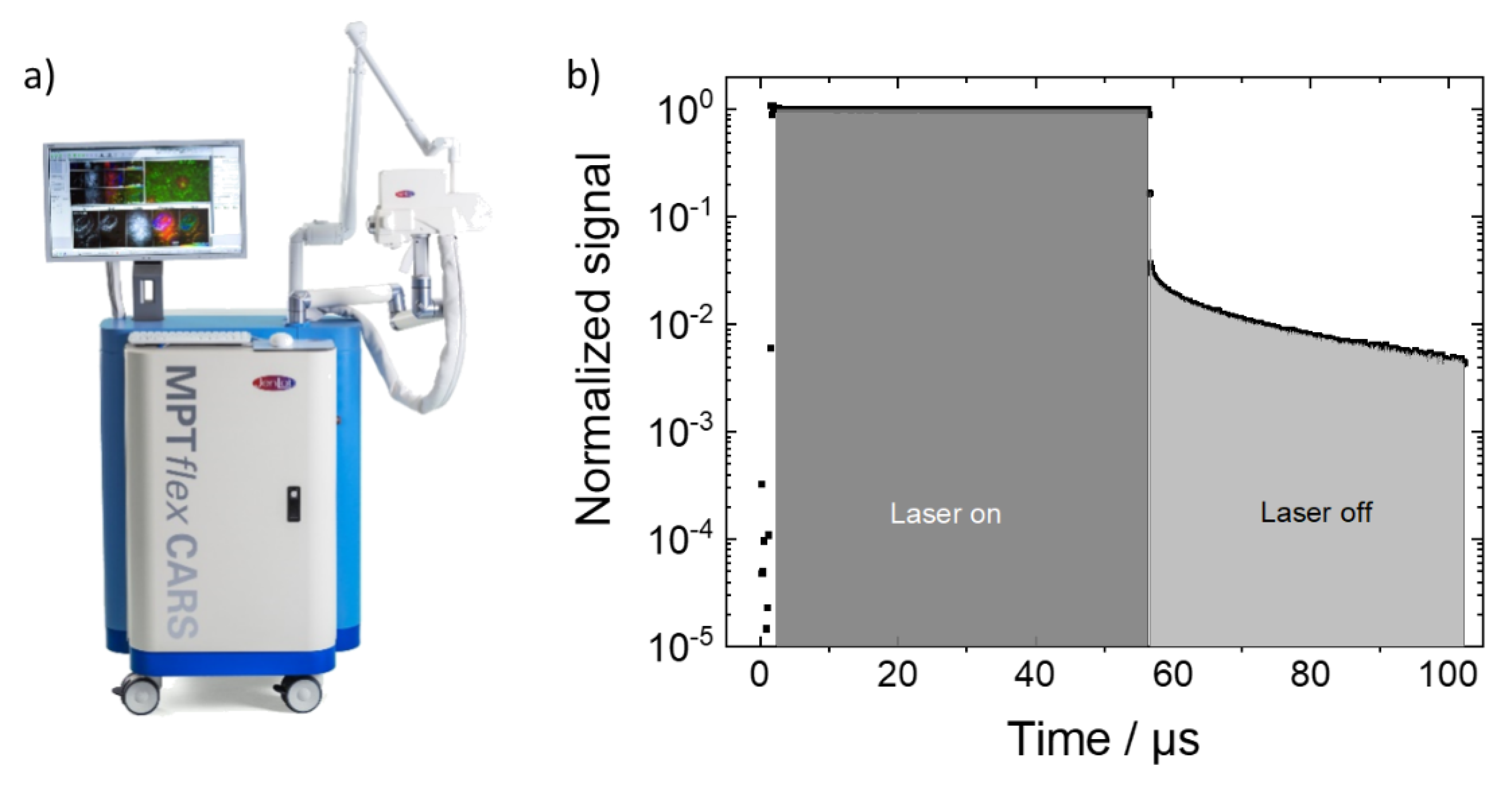
The color changes of bones as a result of temperature are well-known and caused by changes of the chemical composition of the organic components [16]. Figure 2b shows microscopic images which were derived from the pixelwise-collected photon counts during “laser on” and “laser off” times. The laser “on-time” images reflect the fluorescence intensity distribution (with negligible phosphorescence contributions) and the “laser-off times” reflect the phosphorescence signal. Microscopic fine structures of the bone samples can be recognized in both the fluorescence and phosphorescence signals, although, the fluoresce intensity is up to two orders of magnitude higher. For example, the total photon counts were 233 × 10⁶ and 4 × 10⁶ for fluorescence and phosphorescence in the 600 °C images, respectively. For both, the 400 °C- and the 900 °C-heated samples, only fluorescence was detectable. The ratio of the total phosphoresce to fluorescence intensities for the different maximum exposure temperatures is shown in Figure 3.

The figure indicates a clear dependence of the intensity ratio on the exposure temperature. The bone sample which had been subjected to 400 °C hardly phosphorescents. With increasing exposure temperature, the ratio significantly increases up to a maximum of 600 °C from where it drops to 700 °C and 800 °C until at 900 °C the phosphorescence vanishes again. This general trend has been observed with all measured samples, although, different regions of a sample do exhibit varying phosphorescence and fluorescence emission intensities. The temperature dependence of the data in Figure 3 is in line with the trend described by Krap et al. for the phosphoresce intensity scores [3]. The phosphoresce-to-fluorescence ratio is an easy to obtain and more unbiased measure of the phosphorescence, whose absolute intensity is affected by the exact excitation and focusing conditions, without subjective observer evaluation. However, it should be noted that the described temperature dependence of the ratio does not rule out individual temperature dependencies of both the fluorescence as well as the phosphorescence. In fact, our data seems to indicate that absolute intensity values cannot be directly compared for the different samples since they depend on the region of interest and other imaging conditions.

With our measurement setup, the phosphorescence decay can also be analyzed pixelwise. This phosphorescence lifetime microscopy (PLIM) is the phosphorescence analogue of the better-known fluorescent lifetime microscopy (FLIM) [9,10,15]: the time-dependent data are pixelwise color-coded according the to fit parameters. Usually, the day data are fitted by a mono or bi-exponential decay curve. We have used a bi-exponetial fit curve for the decay time tmean = a1 × t1 + a2 × t2 with amplitudes a1,2 (a1 + a2 = 100%) of the short and long decay times t1,2 as fit parameters [9]. For the sample that was exposed to 700 °C (a photo as well as the fluorescence and phosphorescence intensity images are shown in Figure 1), Figure 4 exemplarily shows the corresponding PLIM data with color coding according to values of the decay time components. In the PLIM image in Figure 4a, the short decay time t1 is pseudo-color coded and the pixel brightness corresponds to the photoluminescence intensity. The color coding covers a range between 2 µs (red) and 12 µs (blue) as indicated by the background colors of the histogram (Figure 4b). The t1 histogram has two maxima around 4.5 µs and 10 µs. The decay time data of the phosphorescence for a single pixel is shown in Figure 4c (blue dots) along with the fit curve (solid red line) on a semi-logarithmic scale. The time range covers the “laser off” time between 56 µs and 110 µs as described in Section 2.1. The progression of the measured decay data indicates a bi-exponential decay which is the reason why a fitting with two decay times was applied. The fit parameters for that pixel are shown in Figure 4d. They reveal the fast and slow decay times and the corresponding amplitudes t1 = 5.6 µs and a1 = 54% and t2 = 52.2 µs and a2 = 46%, respectively. The PLIM image with pseudo-color coding of t2 and the corresponding t2 histogram are shown in Figure 4e,f, respectively. The color coding spans the decay-time range from 20 µs (red) up to 60 µs (blue). It exhibits a maximum around 40 µs but is non-zero for the whole covered range. Both PLIM images (Figure 4a,e) exhibit regions with different decay times (compare blue, green, and reddish regions). This could be an indication that different phosphorescent materials with different decay times are present or the microscopic environment affects the phosphorescence decay time. It should be noted, however, that the fitting results are also affected by the choice of fitting conditions like the fitting boundaries. This concerns in particular the absolute values of the fitting parameters but to a much lesser degree the spatial variation of decay times. Further investigations are necessary, which are outside the scope of this paper, to investigate the possible presence as well as the nature of different phosphorescent substances and the influence of artifacts due to the fit conditions and settings.

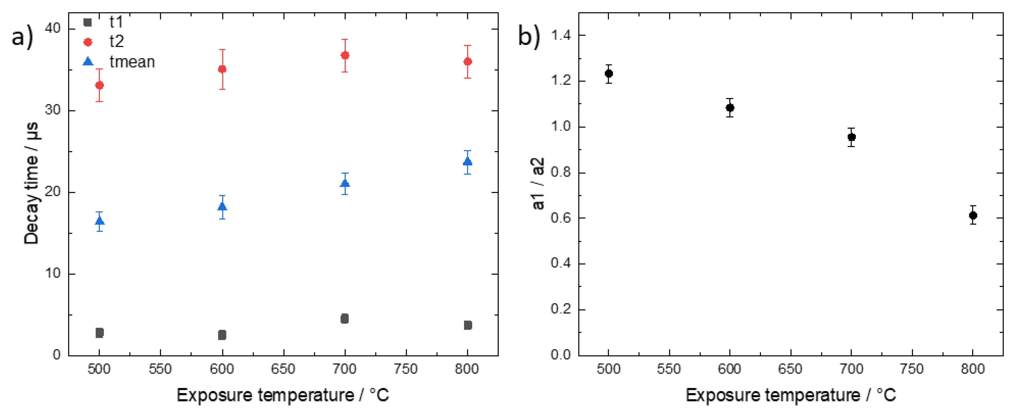
Since we record the time-resolved phosphorescence signals, it is interesting to check for a possible temperature dependence of the decay times. Such a dependence would indicate a change of the type of phosphorescent substance or the microenvironment with exposure temperature. Figure 5 shows data derived from global fit analysis, i.e., by summing the signals from all image pixels for each time channel and fitting the resulting decay time data.

The decay time data were fitted again with a two-exponential decay function. The phosphorescence intensities of the 400 °C and 900 °C samples were too low for a meaningful decay time analysis and, therefore, are not included in Figure 5. While the values of both the fast and slow decay times do not significantly change with increasing temperature, the mean decay time increases from 16 µs to 24 µs. This increase reflects mainly a decrease of the contribution of the fast decay component as depicted in Figure 5b. This could result from a change of the composition of the phosphorescent bone substances. However, more data are needed to clarify and validate this dependence and the possible conclusions which are outside the scope of this paper. The general observation confirms the temperature dependence of the intensity-ratio dependence of Figure 3 and the findings by Krap et at. in the way that, depending on the exposure temperature, the phosphorescent components which give rise to t1 and t2 are either present or absent but not significantly changed further [3].

4. Conclusions

For the first time phosphoresce lifetime microscopy was applied to investigate high-temperature-induced effects on bone samples. The results indicate a strong influence of the maximum exposure temperature on the phosphoresce intensity and a much weaker effect on the lifetime. The simultaneously measured fluorescence allows minimizing observer bias and the influence of experimental conditions by deriving the phosphoresce-to-fluorescence ratio. The microscopic imaging capability allows detecting even microscopic variations of the phosphorescence emission by the bone substance. The results described here, which were obtained with chicken bones, presumably also apply to human bones since the vertebrate bones are composed of the same chemical components [17]. Our findings, although performed on a small sample number, indicate that the introduction of PLIM for the analysis of high-temperature-exposed bone photoluminescence could be a useful tool in improving the current forensic and archeological analysis of bone sample.

References

1. Krap, T.; Nota, K.; Wilk, L.S.; Van De Goot, F.R.W.; Ruijter, J.M.; Duijst, W.; Oostra, R.-J. Luminescence of thermally altered human skeletal remains. Int. J. Leg. Med. 2017, 131, 1165–1177. [Google Scholar] [CrossRef] [PubMed] [Green Version]
2. Lambrecht, G.; Mallol, C. Autofluorescence of experimentally heated bone: Potential archaeological applications and relevance for estimating degree of burning. J. Archaeol. Sci. Rep. 2020, 31, 102333. [Google Scholar] [CrossRef]
3. Krap, T.; Busscher, L.; Oostra, R.-J.; Aalders, M.C.G.; Duijst, W. Phosphorescence of thermally altered human bone. Int. J. Leg. Med. 2021, 135, 1025–1034. [Google Scholar] [CrossRef] [PubMed]
4. Bachman, C.H.; Ellis, E.H. Fluorescence of Bone. Nature 1965, 206, 1328–1331. [Google Scholar] [CrossRef] [PubMed]
5. Harbeck, M.; Schleuder, R.; Schneider, J.; Wiechmann, I.; Schmahl, W.W.; Grupe, G. Research potential and limitations of trace analyses of cremated remains. Forensic Sci. Int. 2011, 204, 191–200. [Google Scholar] [CrossRef] [PubMed] [Green Version]
6. Baggaley, E.; Botchway, S.W.; Haycock, J.W.; Morris, H.; Sazanovich, I.V.; Williams, J.G.; Weinstein, J.A. Long-lived metal complexes open up microsecond lifetime imaging microscopy under multiphoton excitation: From FLIM to PLIM and beyond. Chem. Sci. 2014, 5, 879–886. [Google Scholar] [CrossRef] [Green Version]
7. Kalinina, S.; Breymayer, J.; Schäfer, P.; Calzia, E.; Shcheslavskiy, V.; Becker, W.; Rück, A. Correlative NAD(P)H-FLIM and oxygen sensing-PLIM for metabolic mapping. J. Biophotonics 2016, 9, 800–811. [Google Scholar] [CrossRef] [PubMed]
8. Shcheslavskiy, V.I.; Neubauer, A.; Bukowiecki, R.; Dinter, F.; Becker, W. Combined fluorescence and phosphorescence lifetime imaging. Appl. Phys. Lett. 2016, 108, 091111. [Google Scholar] [CrossRef]
9. Becker, W. The bh TCSPC Handbook; Becker & Hickl: Berlin, Germany, 2019. [Google Scholar]
10. König, K. Review: Clinical in vivo multiphoton FLIM tomography. Methods Appl. Fluoresc. 2020, 8, 034002. [Google Scholar] [CrossRef] [PubMed]
11. Weinigel, M.; Breunig, H.G.; Kellner-Höfer, M.; Bückle, R.; Darvin, M.; Klemp, M.; Lademann, J.; König, K. In vivo histology: Optical biopsies with chemical contrast using clinical multiphoton/coherent anti-Stokes Raman scattering tomography. Laser Phys. Lett. 2014, 11, 055601. [Google Scholar] [CrossRef]
12. Weinigel, M.; Breunig, H.G.; Uchugonova, A.; König, K. Multipurpose nonlinear optical imaging system for in vivo and ex vivo multimodal histology. J. Med. Imaging 2015, 2, 16003. [Google Scholar] [CrossRef] [Green Version]
13. König, K.; Breunig, H.G.; Batista, A.; Schindele, A.; Zieger, M.; Kaatz, M. Translation of two-photon microscopy to the clinic: Multimodal multiphoton CARS tomography of in vivo human skin. J. Biomed. Opt. 2020, 25, 014515. [Google Scholar] [CrossRef] [PubMed]
14. Denk, W.; Strickler, H.; Webb, W. Two-photon laser scanning fluorescence microscopy. Science 1990, 248, 73–76. [Google Scholar] [CrossRef] [PubMed] [Green Version]
15. König, K. Multiphoton Microscopy and Fluorescence Lifetime Imaging; König, K., Ed.; De Gruyter: Berlin, Germany, 2018. [Google Scholar]
16. Rubio, L.; Díaz-Vico, R.; Smith-Fernández, I.; Smith-Fernández, A.; Suárez, J.; Martin-De-Las-Heras, S.; Santos, I. Spectrophotometric Color Measurement to Assess Temperature of Exposure in Cortical and Medullar Heated Human Bones: A Preliminary Study. Diagnostics 2020, 10, 979. [Google Scholar] [CrossRef] [PubMed]
17. Florencio-Silva, R.; Sasso, G.R.d.S.; Sasso-Cerri, E.; Simões, M.J.; Cerri, P.S. Biology of Bone Tissue: Structure, Function, and Factors That Influence Bone Cells. BioMed Res. Int. 2015, 2015, 421746. [Google Scholar] [CrossRef] [PubMed] [Green Version]
Figure 1. (a) Multiphoton imaging system which was modified to incorporate additional PLIM capability as described in the text. (b) Temporal dependence of the recorded signals during the pixel dwell time during which the laser illumination was first on (“laser-on”) and then switched off (“laser-off times”). During the “laser-on time” fluorescence and phosphoresce are generated. The fluorescence quickly fades after the laser illumination is stopped and the slower decaying phosphoresce can be detected background free. The shaded areas indicate the time segments which were summed to yield the fluorescence and phosphoresce counts.
Applsci 12 01066 g001
Figure 2. (a) Photographs of chicken bone samples after being exposed to maximum temperatures between 400 °C and 900 °C. (b) Microscopic photoluminescence images of the different samples. The brightness reflects the intensity of fluorescence (laser on) and phosphorescence (laser off), respectively. Yellow and green pseudo colors were applied to increase the image clarity.
Applsci 12 01066 g002
Figure 3. Ratio of phosphorescence to fluorescence intensities derived from Figure 2b. The line is a guide to the eye only.
Applsci 12 01066 g003
Figure 4. Phosphorescence lifetime imaging and decay time analysis by bi-exponential fitting of the time-resolved phosphoresce signal. (a) PLIM image where the pixel colors represent the value of the fast decay time component t1 which was obtained by pixelwise fitting the time-resolved phosphorescence data. The colors cover values from 2 µs to 12 µs as indicated by the background colors of the histogram in (b). The image shows a region of 100 µm × 100 µm. (b) Color legend and pixel frequency histogram of the fast decay time values. (c) Phosphoresce decay data (blue dots) and fit curve (red line) at the position which is indicated by blue crossing lines in (a). (d) Fit parameters which correspond to the fit curve in (c). (eg) Corresponding results for the slow decay component t2. (h) Fit parameters which correspond to the fit curve in (g).
Applsci 12 01066 g004
Figure 5. (a) Values of fast, slow, and mean decay times obtained by fitting a bi-exponential decay curve to the time-resolved phosphorescence data in dependence of exposure temperature. (b) Ratio of relative amplitudes of the fast (a1) and slow (a2) decay time components. The error bars reflect the range of fit parameters that yield the same goodness of fit.
Applsci 12 01066 g005
Publisher’s Note: MDPI stays neutral with regard to jurisdictional claims in published maps and institutional affiliations.