Abstract
The vigorous development of Time Series Neural Network in recent years has brought many potential possibilities to the application of financial technology. This research proposes a stock trend prediction model that combines Gate Recurrent Unit and Attention mechanism. In the proposed framework, the model takes the daily opening price, closing price, highest price, lowest price and trading volume of stocks as input, and uses technical indicator transition prediction as a label to predict the possible rise and fall probability of future trading days. The research results show that the proposed model and labels designed by this research can effectively predict important stock price fluctuations and can be effectively applied to financial commodity trading strategies.
1. Introduction
Machine Learning (ML) is one of the branches of Artificial Intelligence (AI) [1]. It generally refers to the method of inferring and summarizing data through a certain mathematical rule through a program, and finally obtaining a predictive model [2,3]. Machine learning methods can be divided into supervised learning, unsupervised learning, semi-supervised learning, reinforcement learning, etc., according to whether the data is labeled or not [4,5]. Among many different types of machine learning algorithms, supervised learning is widely used in various classification problems due to its accuracy in target prediction. Common supervised learning algorithms include Genetic Algorithm [6], Bayes Classifier [7], Regression Analysis [8], Support Vector Machine (SVM) [9], Entropy-based method [10], Deep Learning (DL) [11], etc. Nowadays, various deep learning and machine learning algorithms have been widely used in various fields, such as communication networks, QoS Control, 4G/5G communications, Internet of Things and Natural Language Processing [12,13,14,15].
Among various neural network models, Recurrent Neural Network (RNN) [16], Long Short-Term Memory (LSTM) [17], Gate Recurrent Unit (GRU) [18], Attention Mechanism [19] and other time series DNN models are particularly good at processing continuous data, such as natural language processing, machine translation, speech recognition, financial index prediction, etc.
The popularization of financial digitization and the vigorous development of artificial intelligence have also driven the future trends of mobile financial management and new Financial Technology (FinTech). In theoretical research, Nelson [20] proposed the concept of using LSTM Neural Networks to predict the future trend of stocks. The model label is a binary classification: Compared with the previous day’s closing price, the current day’s price is up/down. The experimental targets were four stocks selected from the Brazilian Stock Exchange, and the result achieved a forecast accuracy up to 55.9%.
Chen et al. [21] used the LSTM model to estimate the price trend of WTI Crude Oil. The experiment compared LSTM, deep believe network, Autoregressive Moving Average model (ARMA) model and Random Walk model, and the results showed that the LSTM model is more sensitive to changes in crude oil futures prices.
Fabbr and Moro [22] used the RNN-LSTM model to perform regression and classification analysis for Dow Jones Industrial Average (DJIA). The training data included 2000–2017 Dow Jones Index, and the backtest time included 2009–2017. The results showed that the model predicts the trend can be clearly close to the real material.
Chen et al. [23] proposed an RNN-boost combined with Latent Dirichlet Allocation (LDA) for feature selection of data. The experimental target is the Shanghai–Shenzhen 300 Stock Index (HS300), and the objective function is to predict the ups and downs of the index. The results show that the time series model performs better than other traditional methods, such as Support Vector Regression (SVR) [24].
Li et al. [25] first proposed the MI-LSTM (Multi-Input) prediction model based on the Attention mechanism. In the proposed model, the Attention Layer accepts the output of the LSTM layer, and finally uses Softmax to obtain the index rise and fall prediction results. The target is the Shanghai–Shenzhen CSI 300, which is the top 300 stocks with the largest weights in the Shanghai and Shenzhen stock markets. The results show that the sequence model with the Attention mechanism is better than the general sequence model.
Rui et al. [26] used the DNN, LSTM and CNN models to achieve real-time trading prediction analysis before betting games. The experimental subject is UK Betfair betting exchange, which is the largest betting trader in the UK. Data attributes contained the followings: integral of the price change of the runner and competitor runner, liquidity variation in both ask/bid sides, volume variation and direction. At the theoretical level, LSTM is more suitable for real-time time series analysis and prediction; however, the experimental result shows that CNN achieved higher accuracy in prediction before the betting game.
Feng et al. [27] proposed a new Temporal Graph Convolution (TGC) concept. Given the sequence features of N stocks and the multi-dimensional binary relationship, TGC can relearn and obtain new sequence features. This research combines LSTM and TGC to perform correlation calculation and ranking to weighted stocks and uses this correlation to predict the return on investment of the market. Its research has obtained a very high return on investment in the backtest of NASDAQ and NYSE.
Lee et al. [28] proposed a Deep Q network (DQN) combined with a convolutional neural network. The model takes stock trading volume and closing price graphs as input and is trained on data from different countries. The results show that the proposed model has the characteristic of transfer learning and can be trained on relatively large data and tested on a small market. In terms of return on investment and model adaptability, Feng et al. and Lee et al. are the current state-of-the-art models.
Subsequently, more in-depth network models were applied to different trading markets and financial commodity price predictions [29,30,31,32,33,34]. In our previous research [35], we explored the effectiveness and practicality of various financial analysis technical indicators in the time series deep learning network. This research uses well-known Moving Average (MA) technical indicators to design the feature selection algorithm, and uses the four-layer LSTM to conduct the actual measurement. The experimental target is TWSE 0050 ETF, and the results confirm that the technical indicators can effectively improve the model prediction accuracy in the time series deep network.
Based on the above literature discussion, it can be found that most of the current research on the application of deep network to financial products is mainly based on price forecasting. Most of the models do not use financial technical indicators, nor do they focus on trading strategies. This study introduces technical indicators into the deep neural network, and studies whether the model output is effective as a trading strategy reference directly. This research combines Back-propagation Neural Network, GRU and Attention Mechanism to design a deep learning-based stock trading strategy model, and combines technical indicators for empirical analysis.
The remaining chapters of this study are as follows: The second section discusses time series DNN models, the third section introduces the proposed framework, the fourth section is the experimental results and analysis, and the final section gives the conclusion and future works.
2. Time-Series Deep Neural Networks
This section introduces the deep learning concepts used in this research, including Deep Feedforward Neural Network, Backpropagation Neural Network, Recurrent Neural Network (RNN), Gated Recurrent Unit (GRU), and Attention Mechanism.
2.1. Deep Neural Network
The Deep Neural Network (DNN) simulates the operation of human nerve conduction, using training data to continuously learn and modify the weights between neurons to achieve the correct output. The advantage of neural network over other machine learning algorithms is that it does not need to assume the correlation and relative relationship between input and output parameters. The network itself can automatically learn the deep relationship between the label and each attribute, and rely on the ability of non-linear mapping. The fundamental operation of DNN consists of two parts: (1) Feed-forward Computing and (2) Gradient Back-propagation, which are described as follows:
Given the bias b of each layer, the input vector of the previous layer , the weight vector of the previous layer to the target neuron , the activation function , the feedforward operation generates output based on the input of the previous layer of neurons: , where is the inner product of the weight vector and the input vector . The learning rule of the neural network is mainly to give an error evaluation function with N training samples, DNN obtained the updated weight by the way of gradient-derived transmission by delta rules [36,37,38]:
The error term of the (l + 1)-th layer can be obtained from the weight of the previous layer, and weight and bias update are calculated as follows:
where represents element-wise multiplication, f(•) is the nonlinear transformation equation in a neuron, denotes the weight matrix from l-layer to (l + 1)-layer.
2.2. Recurrent Neural Network (RNN)
Recurrent neural network (RNN) is one of the neural network models. Compared with the fundamental DNN, the calculated output of each hidden layer in DNN can only be passed to the output of the next layer in one direction, and the interrelationships of context cannot be analyzed. RNN transfers the weight of the hidden layer to the next time sequence and can perceive the influence of the data before and after on the current data. Compared with DNN and Convolutional Neural Networks (CNN), RNN is suitable for sequence-related data, such as sentence generation, speech recognition, language translation, stock forecasting, etc. [39,40]. The RNN structure is shown in Figure 1. In this architecture, U, V and W are shared weights. There will be a non-linear transformation from U to the hidden layer. The nonlinear transfer function is usually tanh, and the error function uses Cross Entropy. In addition, the multi-category output is converted through the Softmax Function before V to output.
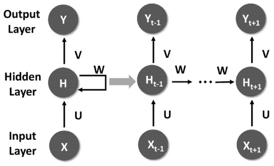
Figure 1.
Fundamental RNN Architecture.
In the RNN architecture, the length of input and output is not fixed and synchronized. Depending on the application category, there can be the following extensions:
- One to one: fixed-length input/output. For example, input the stock price of the day, and output the stock price of the next day.
- One to many: single input, multiple output. For example, take the stock price of the day as the input, and output the estimated stock price in the next few days.
- Many to one: Multiple inputs, single output. For example, input the stock price in a week, and output next week’s stock price.
- Synchronization many to many: Both input and output are multiple. For example, input one week’s stock price and synchronously output the next week’s stock price in real time.
- Asynchronous many to many: Input one week’s stock price, after the input is over, output the next week’s stock price asynchronously.
- Asynchronous sequence-to-sequence (Seq2Seq): This type of input and output are sequence data, and before output is generated, the input message and the code are encoded into a set of context vectors, and the output is to decode the feature vector. The Seq2Seq model can obtain the context dependence of the input more accurately.
2.3. Gated Recurrent Unit (GRU)
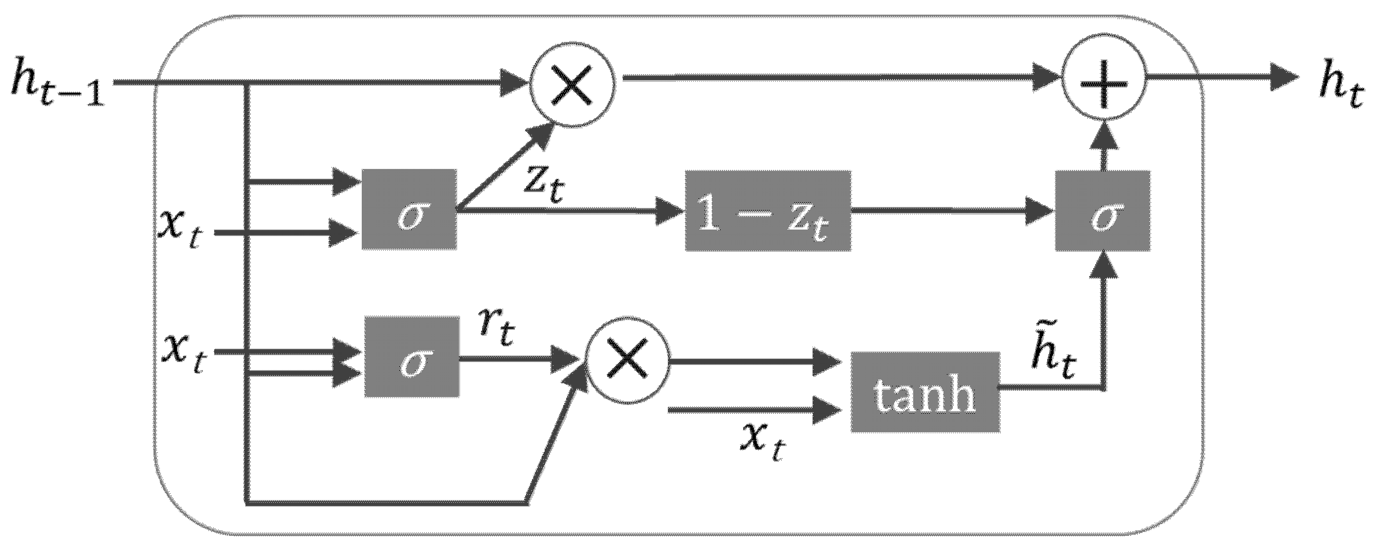
GRU is basically a recurrent neural network. The main difference between GRU and the fundamental RNN is that the memory of RNN will decrease as the data sequence increases. From a theoretical point of view, the gradient feedback of the hidden layer will decrease layer by layer as the sequence data increases. The GRU can effectively improve this problem. GRU Cell is the structure of neurons in a recurrent neural network, as shown in Figure 2. GRU replaces Forget Gate and Input Gate in LSTM with Update Gate, and the intermediate calculation of Cell is as follows:
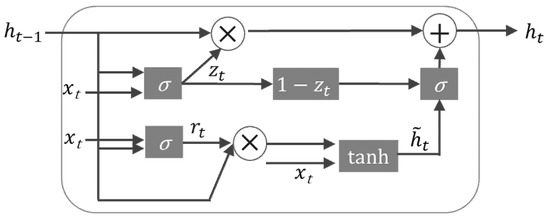
Figure 2.
The GRU Architecture.
Among them, is the Sigmoid Function, is Hyperbolic Tangent Function, represents the Element-wise Product (also known as Hadamard Product), and b is the cell bias. At time t, the state and the input of the previous time t − 1 are passed in, and the two gates: Reset Gate and Update Gate are obtained through . Finally, the element product and tanh are integrated into a new state of −1 to 1, which can simultaneously forget and remember the state. The last update memory integrates and to the next time point. Compared with LSTM operation, GRU has less gateway control and can archive higher performance.
2.4. Attention Mechanism
Attention mechanism was first proposed in the field of computer vision. The Google Mind team applied the Attention mechanism to the RNN model for image classification and achieved extremely high accuracy [41]. Subsequently, Bahdanau and Bengio, the winners of the 2018 Turing Award, applied the Attention mechanism to synchronous machine translation tasks and achieved extremely high performance [42].
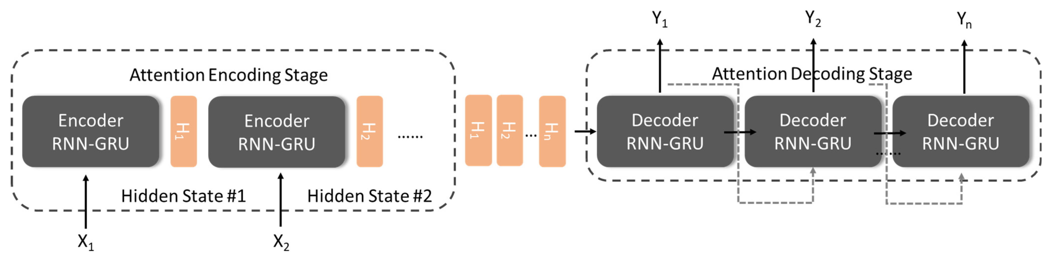
The Attention-based Model is essentially a similarity measure. The more similar the current input and the target state, the greater the weight of the current input, indicating that the current output is more dependent on the current input. Technically, the Attention mechanism is an improved version of the sequence-to-sequence model (Seq2Seq) in RNN. In the Encoding Stage of the traditional time series RNN, the hidden state of each time state is passed forward, and a set of vectors of uniform dimensions are generated before Decoding. This approach results in each training data corresponding to the same set of Context Vector. The Attention mechanism (shown in Figure 3) is aimed at improving this situation. It transmits each hidden state to the back-end decoder, causing the important state in the time period to be learned by the network, that is, the focus of attention.
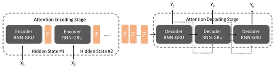
Figure 3.
Encoder–Decoder and Hidden State structure in the attention mechanism.
3. The Proposed GRU-Attention Architecture and Technical Indicators Normalization
3.1. The Proposed GRU-Attention Prediction Model
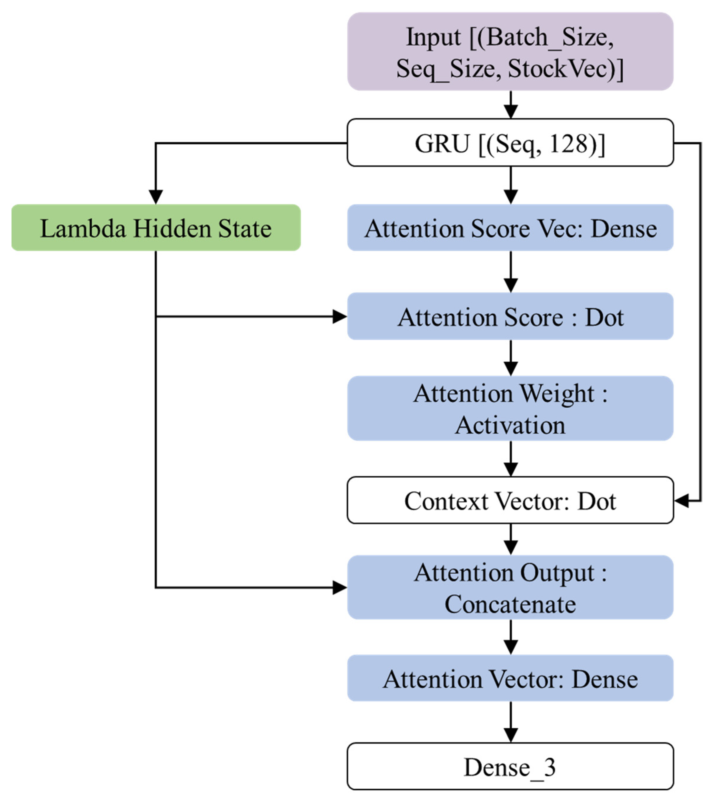
This section introduces the proposed GRU-Attention prediction model. The system architecture of this research is shown in Figure 4. The model input is a set of 3D tensors of time series: the dimensions represent daily transaction data (opening, closing, highest, lowest, and trading volume), time sequence length, and the batch size. The architecture can be regarded as a target function = , where are input tensors, are labels, c represents the context vector. The hidden layer contains a GRU structure of 128 neurons. After outputting to the Attention layer, the Decode vector is generated, and finally the probability of the target category is output by the fully connected layer and the Softmax function.

Figure 4.
The overall architecture of proposed GRU-Attention framework.
As shown in Figure 3, the sequence length and batch size are adjustable parameters, and StockVec is the daily trading attributes of the input stock. The encoder of the model is the GRU-RNN architecture. The GRU receives the input and executes the calculations of Formulas (6)–(9), and then enter the Attention Layer to calculate the context vector of each timestep. This research adopts the Luong style attention [43]; the detailed operations are as follows:
Attention Weights : Use the hidden state of the current decoder to perform a score operation on the hidden states of entire encoder to obtain the importance of to each via Softmax function.
Context Vector : Use attention weight and original to perform weight averaging.
Attention Vector : Concatenation the context vector and decoder of the hidden state and perform nonlinear transformation.
After the encoding vector is generated through GRU-Attention, the latent features are retained through a set of fully connected layers and the class probability is output through Softmax [44], which predicts the probability for the j-th class from input vector :
3.2. Technical Indicators Normalization
Technical Indicators (TI) are indicator data used by investors to implement technical analysis (TA). TAs can simplify market information, such as investor trading intensity, short-term trends, transactions cost, etc., and reflect it on the value or graph to help investors make decisions. This study adopts Relative Strength Index (RSI) [45] and Bias Ratio (BIAS) [46], which are the most commonly used TA tools used by analysts and securities firms, as the estimated stock market signal turning labels to predict the possible ups and downs of future trading days.
3.2.1. The Relative Strength Index (RSI)
The Relative Strength Index (RSI) is a kind of momentum indicator in the stock market. RSI uses the strength of both buyers and sellers as a technical indicator for evaluation, this indicator can be used to analyze the ratio of strengths between buyers and sellers in a certain period of time. The value of RSI ranges from 0 to 100. If RSI > 70–80, it usually means that the market is overheating, and the stock price may fall. RSI < 20–30 means that market transactions have steadily converged and may rebound. This study uses this as the basis for the ups and downs categories, and predicts possible stock price rebounds or turning points in the future trading days. The RSI calculation method is as follows:
Compared with the previous day’s rise, the stock price is set to U, and the fall is set to D. refers to the average increase in n days, and is the average decline in n days. This study takes 20–30 ≤ RSI ≤ 70–80 as the three-category labels, and details will be discussed in the experiment.
3.2.2. Bias Ratio (BIAS)
BIAS uses the moving average as the benchmark and compares it with the intraday price or the closing price of the day to obtain the value of the stock price deviation from the average. The deviation rate can be divided into two categories. “Positive deviation” means that the stock price is above the moving average, and “Negative deviation” means that the stock price is below the moving average. The concept of BIAS is that when the stock price rises sharply and the gap between the moving averages widens, it implies that investors have made a lot of profits, and the stock price will be revised back at any time due to the emergence of selling pressure. When the stock price drops sharply and the gap between the moving averages widens, it implies that investors have suffered heavy losses. After the stock price drops deep, it will attract buyers to enter the market. Therefore, the market will soon rebound. BIAS is usually between +3% and −3%. If it exceeds the set range, the stock price may reverse. Therefore, this study also uses the same benchmark to design three labels of up, down and flat. The BIAS calculation is as follows:
is the deviation rate on n days, Close is the closing price of the day, is the moving average of the closing price on n days. In this study, n is set to 6, 12, 20, and the details will be discussed in the experiment.
3.3. Model Complexity Analysis
This section presents the complexity of the model proposed in this study. In the model complexity analysis of the deep network, the training phase and the testing phase will be discussed separately. In the training phase, let the input sequence length = S, hidden state dimensions = Dh, input dimensions = DI, the time complexity for one gradient step in GRU is O(SDh2 + SDhDI) according to [47] and Equations (1)–(9). The Attention layer takes the input vector d directly from GRU layer; thus, the complexity of Attention layer is O(S2d). The total complexity of the proposed model would be O(SDh2 + SDhDI + S2d) according to the selected sequence length, hidden state dimensions, and input attribute dimensions. In the testing phase, since the feedforward of the neural network is a linear operation, the time complexity is O(1).
4. Experimental Results and Analysis
4.1. Experimental Environment Settings
The experimental environment of this research uses Asus Esc8000 G3 Host, Xeon E5-2600 v3 processor, 4 GB memory, NVIDIA GeForce GTX 1080 ti × 8 GPUs with Ubuntu 18.04 LTS OS. The research target is Taiwan Semiconductor Manufacturing Co., Ltd. (TSMC, code TPE:2330), and the experimental range is selected from 4 January 2016 to 11 May 2021, with a total of 1300 trading days, and the data source is taken from public information of Taiwan Stock Exchange (TWSE). Considering that the stock trading attribute used in this study is in days, the total trading days are not many. To avoid potential underfitting, the proportion of training data is increased in the experimental settings. In this study, 70% of the data was set as the training set, 20% as the validation set, and 10% as the test set. The model is trained for 50–200 Epochs, the batch size is uniformly set to 32, and finally the weight with the highest validation accuracy is used as the prediction model. The measures used in this study are Recall, Precision, F1 and Accuracy:
where TP, TN, FP and FN represent the True Positive, True Negative, False Positive and False Negative, respectively. F1 measure is the is the harmonic mean of Recall and Precision. In the presentation of the experimental results, Recall can show the ratio of the actual categories that are successfully predicted, and Precision shows the proportion of successful predictions in the prediction results. The accuracy can perform an overall evaluation of the correct and incorrect prediction results. In addition, to explore potential causes of mispredictions in multi-class predictions, the resulting presentation will include confusion matrices to clearly depict the mispredicted classes. The loss function uses categorical cross entropy, which is defined as follows:
where n is the number of samples, m is the number of categories.
4.2. Experimental Result of the Relative Strength Index
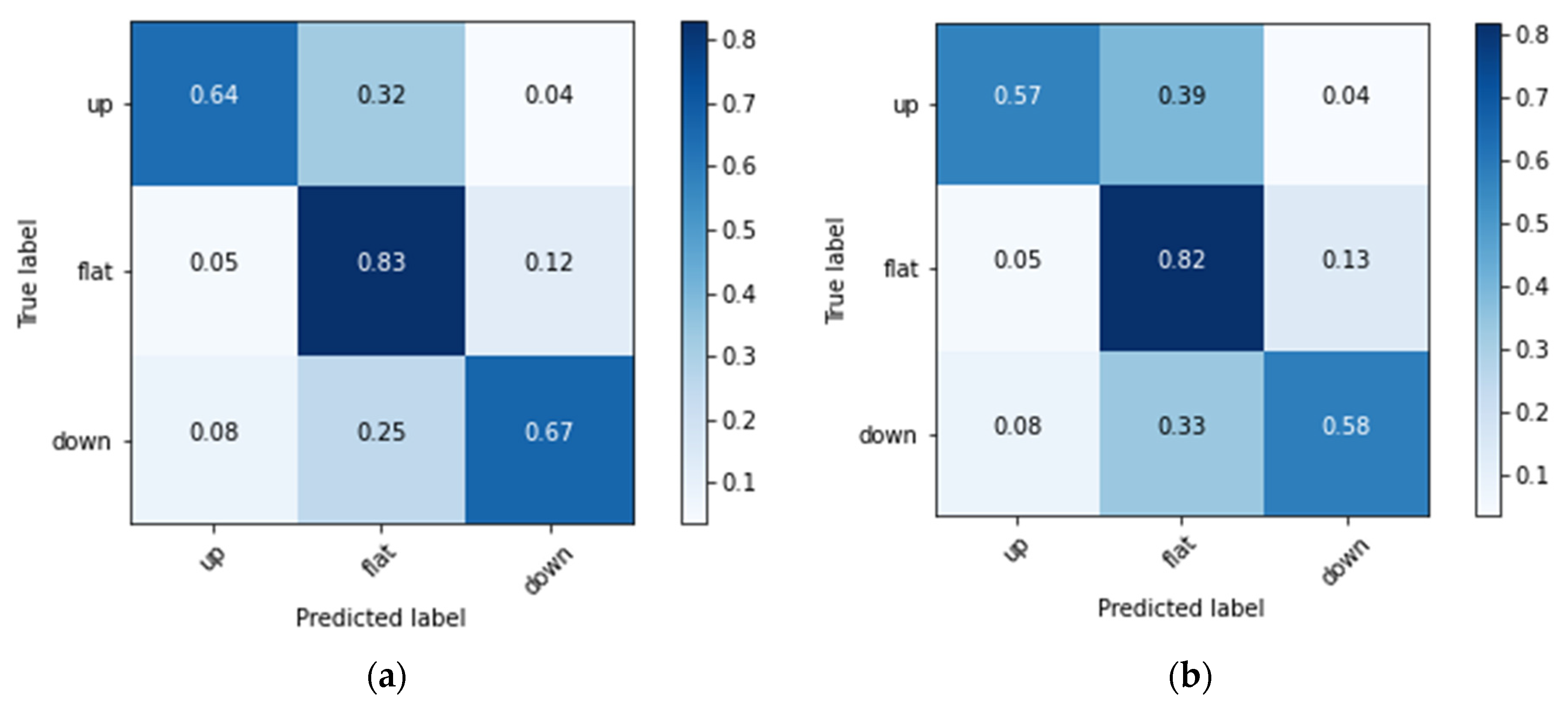
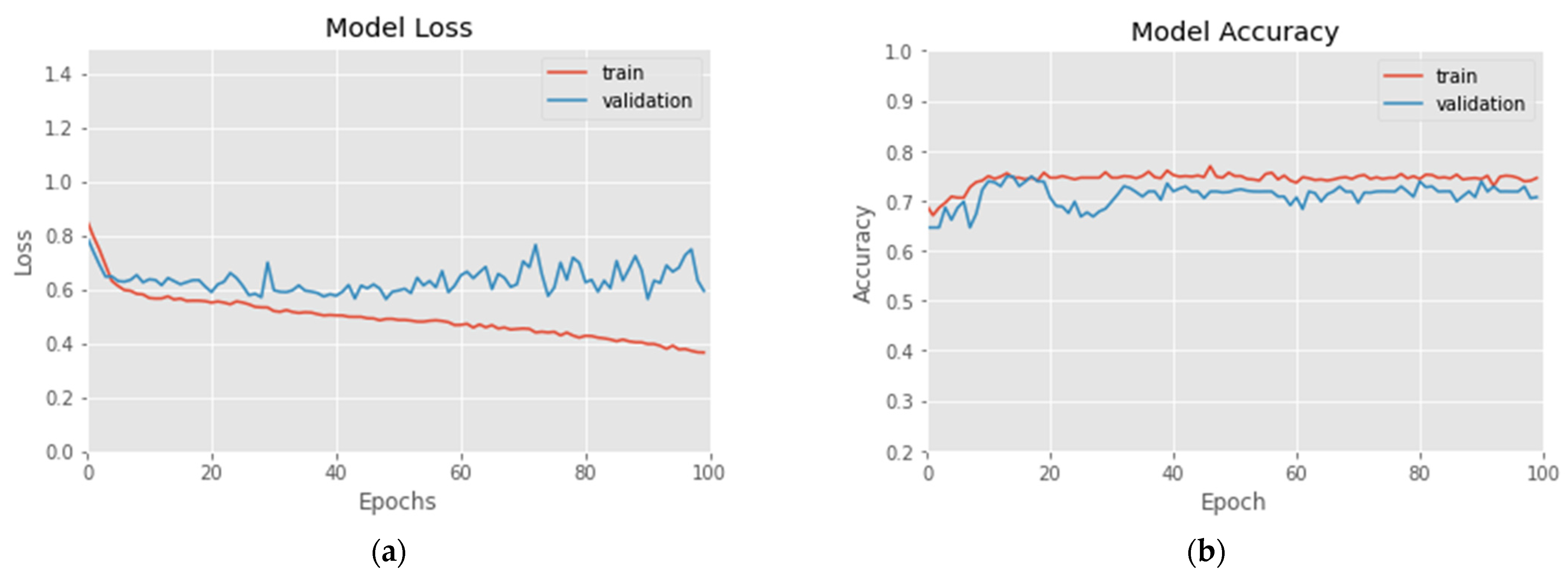
In this experiment, according to Formulas (15) and (16), three labels of prince rising (Up), prince falling (Down) and flat (Flat) are set for 20–80 RSI and 30–70 RSI, respectively. The experimental results are shown in Figure 5 and Figure 6 and Table 1. Figure 5a demonstrates the 100 epochs versus model loss, while Figure 5b shows the data of training accuracy at 100 epochs. Table 1 and Figure 6 show the Recall, Precision, F1, average Accuracy and Confusion Matrix of three categories in the test set. During the training process, the loss of the training data decreases steadily, but the loss of the verification data converges at about 10–20 epochs, and increases when it exceeds 80 epochs, indicating that too many training epochs may cause the model to overfit. The result in Figure 6a shows that in 20_80_RSI, most of the ‘Flat’ category can be correctly predicted, but a certain proportion of ‘Up’ and ‘Down’ categories will be misjudged as ‘Flat’. It can be clearly seen from the experimental result in Figure 6b that, compared with 20_80_RSI, 30_70_RSI has a slightly lower proportion of false positives for the ‘Up’ and ‘Down’ categories. The experimental results show that the estimated accuracy of the 20–80 RSI in three categories is 79.2%, which is higher than 76.4% of the 30–70 RSI. In the data of Recall, Precision and F1 measure, 20–80 RSI is also slightly better than 30–70 RSI. Among them, Precision and Recall in the ‘Flat’ category reach up to 91.3% and 83.2%. In the three categories of predictions, the ‘Flat’ prediction performs best, and the ‘Up’ and ‘Down’ prediction has a phenomenon of misjudgment of each other in few cases. In addition, the Recall of the proposed model is between 64.2% and 83.2%, and the average is 71.66%, which means that more than 70% of the turning signals can be correctly estimated.
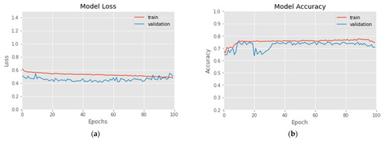
Figure 5.
(a) Loss vs. 100-epochs and (b) Accuracy vs. 100-epochs of 20_80_RSI-labeled training data.

Figure 6.
The Confusion Matrices of (a) 20 ≤ RSI ≤ 80, and (b) 30 ≤ RSI ≤ 70.

Table 1.
Precision, Recall, F1 Measure and Accuracy of the RSI TI.
4.3. Experimental Result of the Bias Ratio
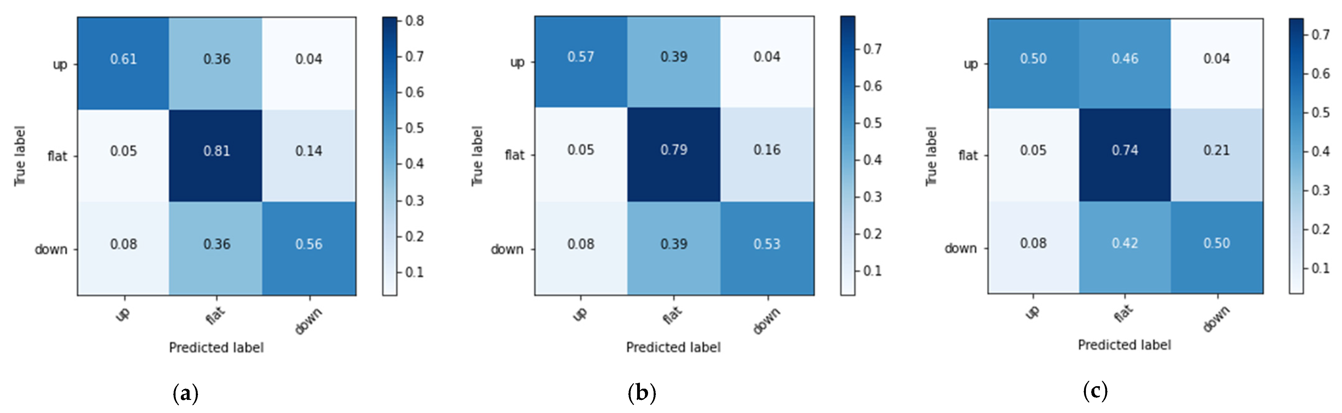
In this experiment, three labels of prince rising (Up), prince falling (Down) and flat (Flat) are set for 6, 12 and 20 BIAS according to Formula (17). The experimental results are shown in Figure 7 and Figure 8 and Table 2. Figure 7a demonstrates the variation of model loss at 100 epochs. Figure 7b shows the accuracy variation at 100 epochs. Table 2 shows the Recall, Precision, F1 measure and average Accuracy of the 6, 12 and 20 BIAS. Figure 8a–c demonstrates the Confusion Matrices of the 6, 12 and 20 BIAS, respectively. In this experiment, the loss of the training data decreased rapidly within 10 epochs, and then showed a steady downward trend. The loss of the validation data converged at about 10–20 epochs. In Figure 8a–c, 6 BIAS has higher prediction accuracy than 12 BIAS and 20 BIAS. However, similar to RSI, most of the misjudgments of ‘Up’ and ‘Down’ are misjudged as ‘Flat’. The reason is probably that ‘Flat’ is the most common case in stock market trading, and its data volume is also greater than the sum of the ‘Up’ and ‘Down’ categories. In summary, the forecast accuracy of 6 days BIAS is 75.6%, which is slightly higher than BIAS based on 12 days, and a large extent better than 20 days BIAS. The average Recall and Precision of 6 BIAS in the three categories are higher than 12 BIAS and 20 BIAS. Twenty days is roughly equivalent to one month trading. Considering the adaptability of the deep network, the results show that long-term BIAS statistics did not increase the accuracy of predictions. Similar to RSI, BIAS’s estimates are mostly correct for the ‘Flat’ label, with Precision and Recall reaching up to 87.2% and 81.4%, and 84.2% in F1 Measure.

Figure 7.
(a) Loss vs. 100-epochs and (b) Accuracy vs. 100-epochs of 6 BIAS-labeled training data.
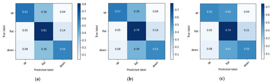
Figure 8.
The Confusion Matrices of (a) 6 days BIAS, (b) 12 days BIAS, and (c) 20 days BIAS.
Table 2.
Precision, Recall, F1 Measure and Accuracy of the BIAS TI.
4.4. Experimental Results of Applying to Backtest of Trading Strategies
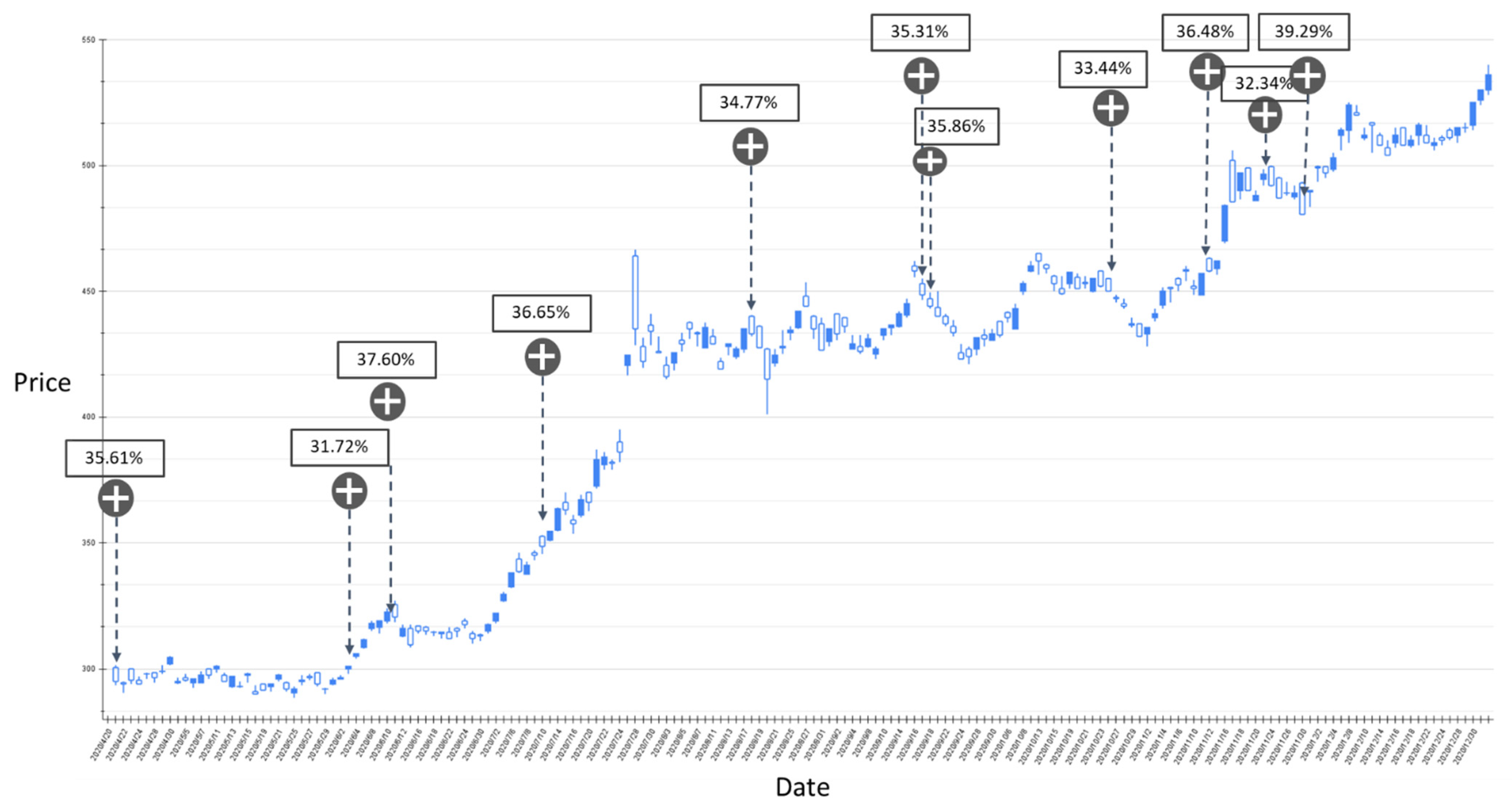
Based on the above experiments, it can be found that the prediction performance of the proposed model for RSI technical indicators is slightly higher than that of BIAS. However, a certain number of labels that are rising or falling are misjudged to be flat. From the perspective of the deep network classification model, the prediction category is limited by the output of Softmax. Therefore, the proposed GRU-Attention model subsequently derives the probability output of Softmax as a reference for investors’ trading strategies. In this study, the stock price fluctuations of TSMC between 20 April 2020 and 5 May 2021 were backtested based on the parameters with higher accuracy in the aforementioned experiments, and set the rising probability value greater than a certain threshold as the estimated buying point. The results are shown in Figure 9, Figure 10, Figure 11, Figure 12, Figure 13, Figure 14 and Figure 15.
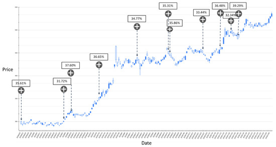
Figure 9.
The RSI-label backtest result of the stock market entry point where the predicted increase probability is between 30% and 40%. Target: TPE:2330, trading interval: 20 April 2020–30 December 2020.
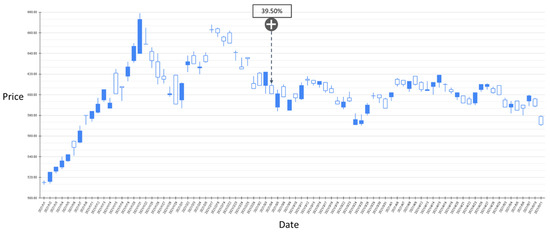
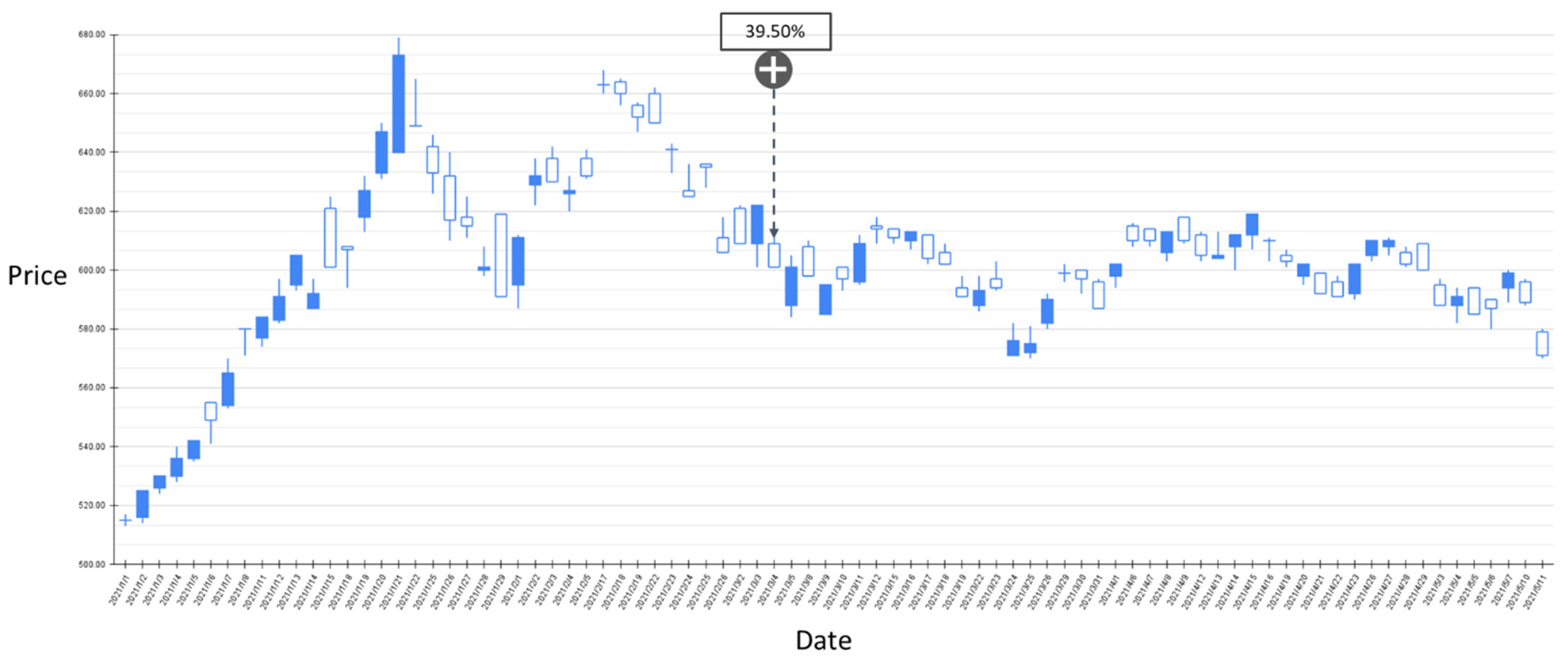
Figure 10.
The RSI-label backtest result of the stock market entry point where the predicted increase probability is between 30% and 40%. Target: TPE:2330, trading interval: 1 January 2021–11 May 2021.
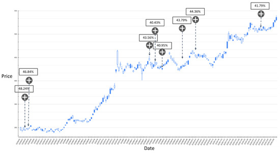
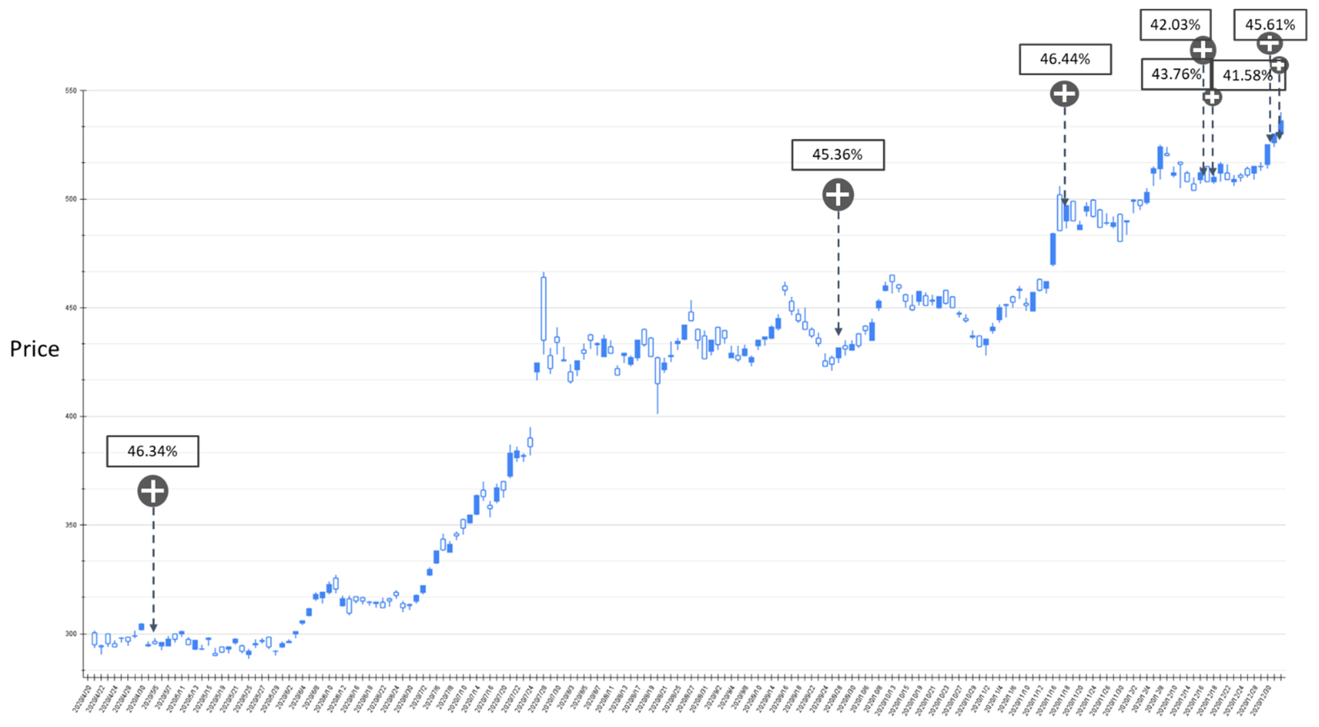
Figure 11.
The RSI-label backtest result of the stock market entry point where the predicted increase probability is greater than 40%. Target: TPE:2330, trading interval: 20 April 2020–30 December 2020.
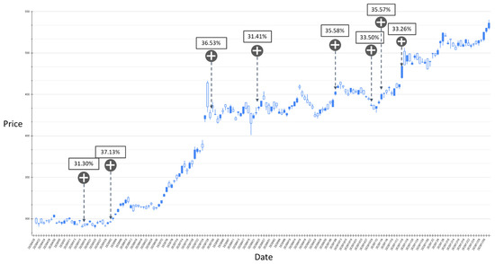
Figure 12.
The BIAS-label backtest result of the stock market entry point where the predicted increase probability is between 30% and 40%. Target: TPE:2330, trading interval: 20 April 2020–30 December 2020.

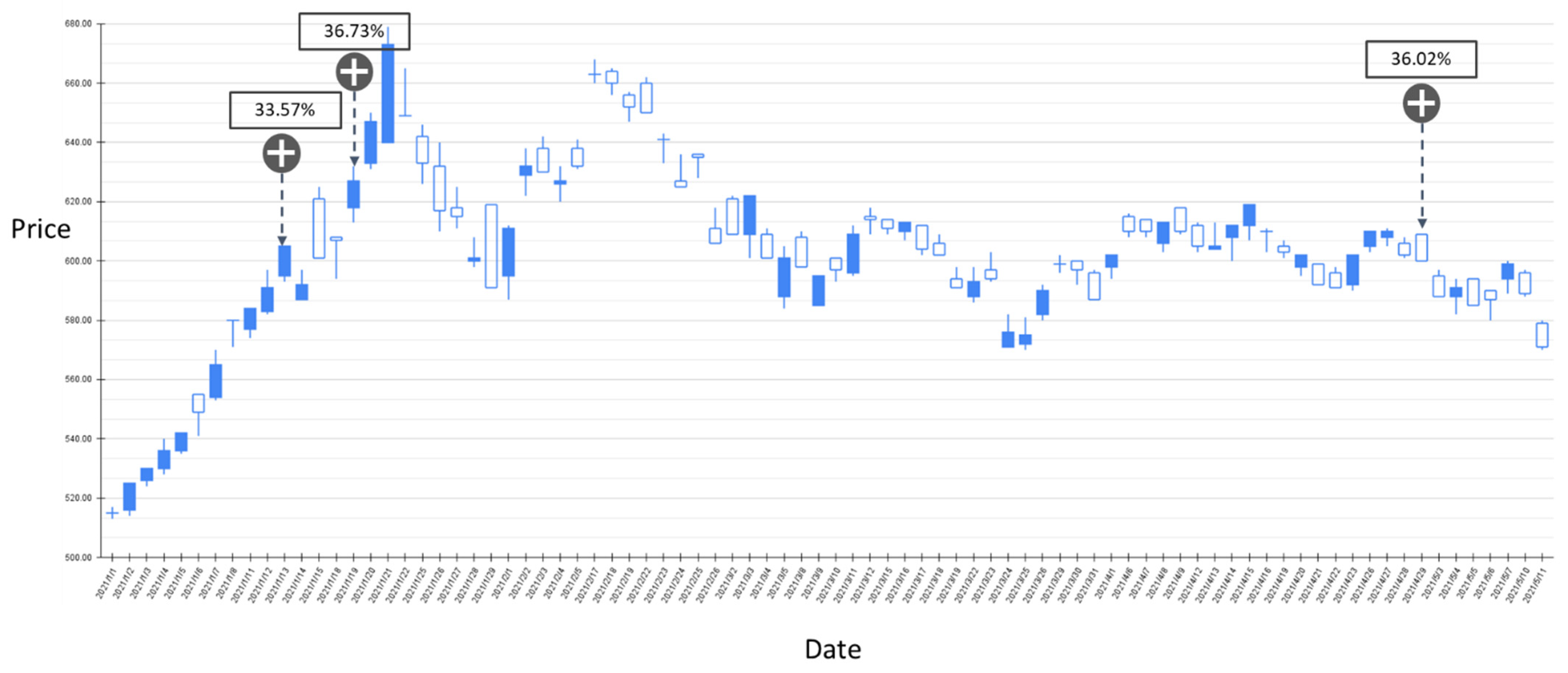
Figure 13.
The BIAS-label backtest result of the stock market entry point where the predicted increase probability is between 30% and 40%. Target: TPE:2330, trading interval: 1 January 2021–11 May 2021.
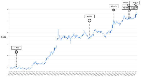
Figure 14.
The BIAS-label backtest result of the stock market entry point where the predicted increase probability is greater than 40%. Target: TPE:2330, trading interval: 20 April 2020–30 December 2020.

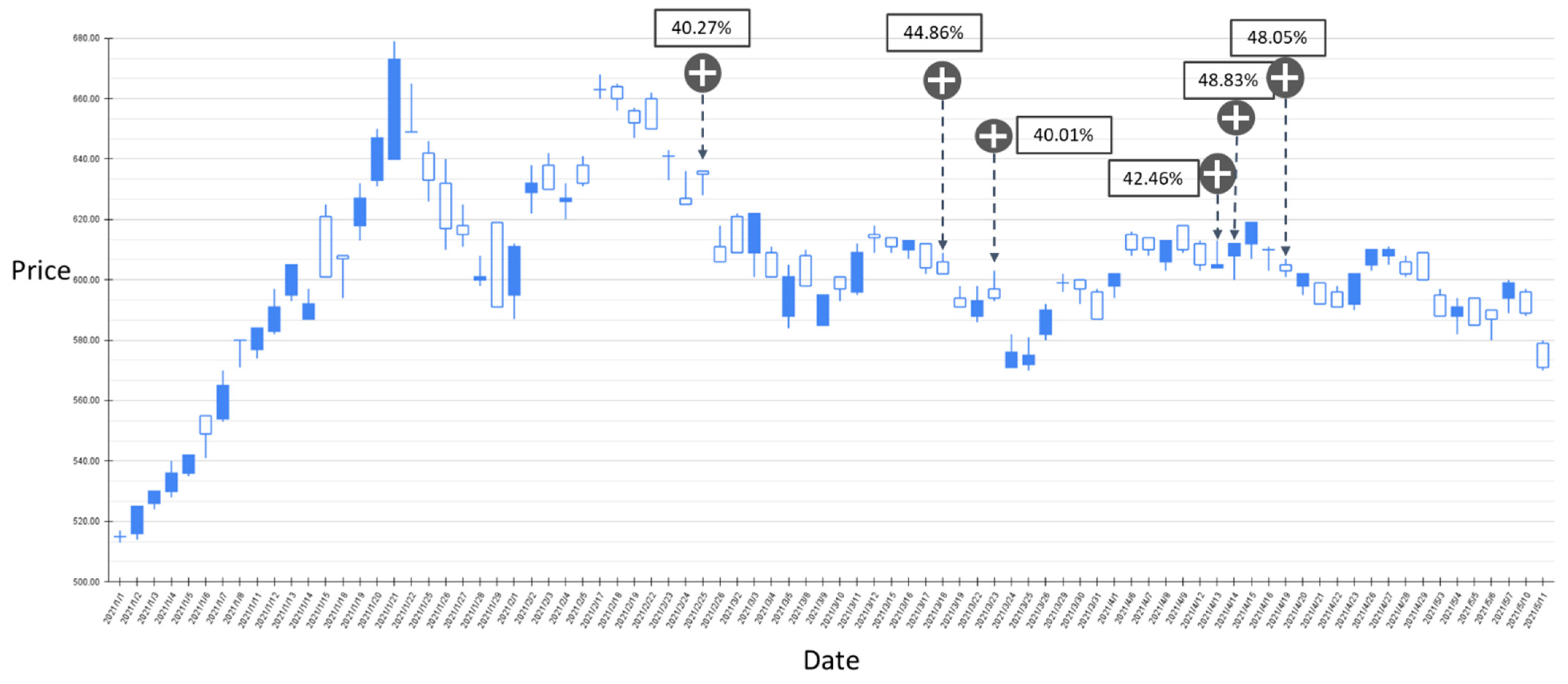
Figure 15.
The BIAS-label backtest result of the stock market entry point where the predicted increase probability is greater than 40%. Target: TPE:2330, trading interval: 1 January 2021–11 May 2021.
Figure 9 shows the results of the experiment where the probability of RSI turning upward is between 30% and 40%, and the trading range is between 20 April 2020 and 30 December 2020. The model has a total of 11 suggestions for stock market entry points in the interval. Figure 10 shows the results of the transaction date 1 January 2021–11 May 2021, and there is only one forecast with an increase probability within 30–40%. The volatility of stocks from March to May in 2021 slows down, and the model also yields reasonable predictions. The volatility between April 2020 and January 2021 is relatively large, and the proposed model also gives relatively more positive market entry estimates value. Figure 11 shows the results of the experiment where the probability of RSI turning upward is greater than 40%, and the trading range is between 20 April 2020 and 30 December 2020. During this time period, the GRU-Attention model suggested a total of eight entry points. Compared with the previous experiment, using a 40% increase probability as the trading time point can more effectively ensure a positive return on investment. In addition, in the experiment of the RSI label, there is no more than 40% increase prediction probability in the interval between 1 January 2021 and 11 May 2021.
Figure 12 and Figure 13 show the results of the experiment where the probability of BIAS turning upward is between 30% and 40% with trading intervals 20 April 2020–30 December 2020 and 1 January 2021–11 May 2021, respectively. In the entire experimental interval, the proposed GRU-Attention model produced a total of 11 market entry opportunities. In the results of this experiment, most of the entry points are relatively low points in the entire stock band. Figure 14 and Figure 15 depict the results of the experiment where the probability of BIAS turning upward is greater than 40%, with trading intervals 20 April 2020–30 December 2020 and 1 January 2021–11 May 2021, respectively. In this time interval, there are 13 prediction results with an estimated increase probability greater than 40%. The forecast results in the 20 April 2020–30 December 2020 interval can obtain positive investment returns, and a few of the forecast results from 1 January 2021 to 11 May 2021 have not obtained positive returns in a short period of time.
Based on the above experimental results, it can be found that using RSI and BIAS as the labels for model training can achieve an average accuracy of more than 70% in classification. The average prediction accuracy with the RSI is higher than the BIAS. However, in importing the model into the trading strategy, the results show that the timing point of BIAS’s estimation is relatively stable. In the result of the estimated stock price increase, there are fewer short-term declines.
4.5. Experimental Results Compared to the State-of-the-Art Models and Traditional Methods
In this section, we compare the model proposed in this research with other methods, including state-of-the-art models [27,28]. Other commonly used machine learning models, including k-nearest neighbors algorithm (KNN), SVM and Random Forest [48], are also included. The above machine learning methods are commonly used in numerical data classification problems. This study incorporates these models to explore their effectiveness for time series classification problems. The source codes of [27,28] are provided in the original papers, other approaches are implemented by this research. In the experimental setting of [27], we selected 20 electronic stocks on the Taiwan Stock Exchange as the related stocks of the target TPE:2330. The positive rate of return is estimated to price up, and vice versa. In the experimental setting of [28], we adopted the CNN module with price volume chart for training. The experimental results are shown in Table 3.
Table 3.
Comparison of the Precision, Recall, F1 Measure and Accuracy. GRU-Att_B and GRU-Att_R represent the BIAS and RSI TIs, respectively.
It can be seen from Table 3 that the architecture of GRU_ATT with technical indicators proposed by this research, has a significant improvement in overall performance compared with other algorithms. The BIAS normalization approach has an improvement of 7.62% and 11.38% in the accuracy measure compared to [27,28], and the RSI approach has an improvement of 4.02% and 7.78%, respectively. Among other machine learning methods, KNN performs better and has a prediction accuracy close to 70%, while Random Forest does not reach 60%. In the algorithms compared in this study, most models have low precision and recall for price increases and declines, which indicates that these models are less sensitive to time series data.
4.6. Experimental Results of Applying to Top 10 Weighted Stocks in TWSE
To verify the effectiveness and scalability of the proposed framework, we retrained the proposed model and calculates the accuracy for TWSE Top 10 weighted stocks: Taiwan Semiconductor Manufacturing Co., Ltd. (TPE:2330), MediaTek Inc. (TPE: 2454), Hon Hai Precision Industry Co., Ltd. (TPE:2317), Formosa Petrochemical Corporation (TPE:6505), Chunghwa Telecom (TPE:2412), Fubon Financial Holding Co., Ltd. (TPE:2881), Cathay Financial Holding Co., Ltd. (TPE:2882), United Microelectronics Corporation (TPE:2303), Evergreen Marine Corporation (TPE:2603), and Delta Electronics, Inc. (TPE:2308). Except for TPE:2330, other models were trained with basic volume and price attributes to compare the differences with and without technical indicators. The results are shown in Table 4. The experimental results show that the accuracy of the model can still reach nearly 70% even without the use of technical indicators. Among all the forecast results, the recall/precision with a flat forecast is the highest, and there are individual differences in other categories.
Table 4.
Precision, Recall, F1 Measure and Accuracy of the top 10 weighted stocks in TWSE.
5. Conclusions and Future Works
This research proposes a GRU-Attention deep neural network as a strategic reference for stock trading. With the theoretical assistance of technical indicators, the effectiveness of the deep network for forecasting financial commodity trends is not limited to the accuracy of the forecast, and the probability of the forecast category can be directly applied to the design of stock market trading strategies. The experimental target is Taiwan Semiconductor Manufacturing Co., Ltd. (TSMC, TPE:2330), which is currently the world’s largest foundry semiconductor manufacturer. The model uses the stock price data of 4 January 2016–11 May 2021 for training and testing, and the price of 20 April 2020–11 May 2021 for trading strategy backtesting. The main contributions of this study are summarized as follows:
- Famous financial commodity analysis tools such as Relative Strength Index and Bias Ratio can effectively assist the prediction accuracy of time series neural networks.
- Taking the TPE: 2330 as an example, the proposed GRU-Attention model can achieve an average prediction accuracy of more than 70%.
- With the aid of RSI and BIAS TIs, the rising points predicted by the model can be positively paid in most cases.
- Compared with other deep network and non-deep network models, the proposed approach has a significant performance improvement in prediction accuracy.
The limitation of the conclusions of this study lies in the use of RSI and BIAS technical indicators, which are combined in the GRU + Attention model. If other technical indicators are used, the indicator normalization method must be redesigned and retrained. The future works of this research include the following:
- Extend the concepts proposed in this study to other non-sequential networks, such as CNN, Transformer, etc.
- Apply the proposed model to other types of financial products, such as futures, options, day trading, etc.
- Extend the deep learning trading strategies to the investment portfolio of different financial products.
- Future research on the use of deep networks for trading strategies can be extended to investment portfolios.
- Cryptocurrency is a popular commodity in the current investment market, and this research can be extended to the analysis of cryptocurrency trends.
Funding
This paper is supported by the Ministry of Science and Technology (MOST) under MOST 110-2221-E-130-008.
Data Availability Statement
Not applicable.
Acknowledgments
The author would like to thank the Ministry of Science and Technology (MOST) for their support during this study.
Conflicts of Interest
The authors declare no conflict of interest.
References
- Samuel, A.L. Some studies in machine learning using the game of checkers. IBM J. Res. Dev. 1959, 3, 210–229. [Google Scholar] [CrossRef]
- Mohri, M.; Rostamizadeh, A.; Talwalkar, A. Foundations of Machine Learning; MIT Press: Cambridge, MA, USA, 2018. [Google Scholar]
- Jordan, M.I.; Mitchell, T.M. Machine learning: Trends, perspectives, and prospects. Science 2015, 349, 255–260. [Google Scholar] [CrossRef] [PubMed]
- Chapelle, O.; Scholkopf, B.; Zien, A. Semi-supervised learning (chapelle, o. et al., eds.; 2006) [book reviews]. IEEE Trans. Neural Netw. 2009, 20, 542. [Google Scholar] [CrossRef]
- Kaelbling, L.P.; Littman, M.L.; Moore, A.W. Reinforcement learning: A survey. J. Artif. Intell. Res. 1996, 4, 237–285. [Google Scholar] [CrossRef] [Green Version]
- Eiben, A.E.; Raue, P.E.; Ruttkay, Z. Genetic algorithms with multi-parent recombination. In International Conference on Parallel Problem Solving from Nature; Springer: Berlin/Heidelberg, Germany, 1994; pp. 78–87. [Google Scholar]
- Spirtes, P.; Glymour, C.N.; Scheines, R.; Heckerman, D. Causation, Prediction, and Search; MIT Press: Cambridge, MA, USA, 2000. [Google Scholar]
- Fotheringham, A.S.; Brunsdon, C.; Charlton, M. Geographically Weighted Regression: The Analysis of Spatially Varying Relationships; John Wiley & Sons: Hoboken, NJ, USA, 2003. [Google Scholar]
- Cortes, C.; Vapnik, V. Support-vector networks. Mach. Learn. 1995, 20, 273–297. [Google Scholar] [CrossRef]
- Safavian, S.R.; Landgrebe, D. A survey of decision tree classifier methodology. IEEE Trans. Syst. Man Cybern. 1991, 21, 660–674. [Google Scholar] [CrossRef] [Green Version]
- Goodfellow, I.; Bengio, Y.; Courville, A. Deep Learning; MIT Press: Cambridge, MA, USA, 2016. [Google Scholar]
- Huang, X.L.; Ma, X.; Hu, F. Machine learning and intelligent communications. Mob. Netw. Appl. 2018, 23, 68–70. [Google Scholar] [CrossRef] [Green Version]
- Huang, X.L.; Tang, X.; Huan, X.; Wang, P.; Wu, J. Improved KMV-cast with BM3D denoising. Mob. Netw. Appl. 2018, 23, 100–107. [Google Scholar] [CrossRef]
- Adi, E.; Anwar, A.; Baig, Z.; Zeadally, S. Machine learning and data analytics for the IoT. Neural Comput. Appl. 2020, 32, 16205–16233. [Google Scholar] [CrossRef]
- Loey, M.; Manogaran, G.; Taha, M.H.N.; Khalifa, N.E.M. A hybrid deep transfer learning model with machine learning methods for face mask detection in the era of the COVID-19 pandemic. Measurement 2021, 167, 108288. [Google Scholar] [CrossRef] [PubMed]
- Mikolov, T.; Karafiát, M.; Burget, L.; Černocký, J.; Khudanpur, S. Recurrent neural network based language model. In Proceedings of the Eleventh Annual Conference of the International Speech Communication Association, Chiba, Japan, 26–30 September 2010. [Google Scholar]
- Hochreiter, S.; Schmidhuber, J. Long short-term memory. Neural Comput. 1997, 9, 1735–1780. [Google Scholar] [CrossRef]
- Cho, K.; Van Merriënboer, B.; Gulcehre, C.; Bahdanau, D.; Bougares, F.; Schwenk, H.; Bengio, Y. Learning phrase representations using RNN encoder-decoder for statistical machine translation. arXiv 2014, arXiv:1406.1078. [Google Scholar]
- Vaswani, A.; Shazeer, N.; Parmar, N.; Uszkoreit, J.; Jones, L.; Gomez, A.N.; Kaiser, L.; Polosukhin, I. Attention is all you need. Adv. Neural Inf. Process. Syst. 2017, 2017, 5998–6008. [Google Scholar]
- Nelson, D.M.; Pereira, A.C.; de Oliveira, R.A. Stock market’s price movement prediction with LSTM neural networks. In Proceedings of the 2017 International Joint Conference on Neural Networks (IJCNN), Anchorage, AL, USA, 14–19 May 2017; pp. 1419–1426. [Google Scholar]
- Chen, Y.; He, K.; Tso, G.K. Forecasting crude oil prices: A deep learning based model. Procedia Comput. Sci. 2017, 122, 300–307. [Google Scholar] [CrossRef]
- Fabbri, M.; Moro, G. Dow Jones Trading with Deep Learning: The Unreasonable Effectiveness of Recurrent Neural Networks. Data 2018, 2018, 142–153. [Google Scholar]
- Chen, W.; Yeo, C.K.; Lau, C.T.; Lee, B.S. Leveraging social media news to predict stock index movement using RNN-boost. Data Knowl. Eng. 2018, 118, 14–24. [Google Scholar] [CrossRef]
- Cakra, Y.E.; Trisedya, B.D. Stock price prediction using linear regression based on sentiment analysis. In Proceedings of the 2015 International Conference on Advanced Computer Science and Information Systems (ICACSIS), Depok, Indonesia, 10–11 October 2015; pp. 147–154. [Google Scholar]
- Li, H.; Shen, Y.; Zhu, Y. Stock price prediction using attention-based multi-input LSTM. In Proceedings of the Asian Conference on Machine Learning, PMLR, Nagoya, Japan, 14–16 November 2018; pp. 454–469. [Google Scholar]
- Gonçalves, R.; Ribeiro, V.M.; Pereira, F.L.; Rocha, A.P. Deep learning in exchange markets. Inf. Econ. Policy 2019, 47, 38–51. [Google Scholar] [CrossRef]
- Feng, F.; He, X.; Wang, X.; Luo, C.; Liu, Y.; Chua, T.S. Temporal relational ranking for stock prediction. ACM Trans. Inf. Syst. 2019, 37, 1–30. [Google Scholar] [CrossRef] [Green Version]
- Lee, J.; Kim, R.; Koh, Y.; Kang, J. Global stock market prediction based on stock chart images using deep Q-network. IEEE Access 2019, 7, 167260–167277. [Google Scholar] [CrossRef]
- Nabipour, M.; Nayyeri, P.; Jabani, H.; Mosavi, A.; Salwana, E. Deep learning for stock market prediction. Entropy 2020, 22, 840. [Google Scholar] [CrossRef] [PubMed]
- Ha, D.A.; Liao, C.H.; Tan, K.S.; Yuan, S.M. Deep Learning Models for Predicting Monthly TAIEX to Support Making Decisions in Index Futures Trading. Mathematics 2021, 9, 3268. [Google Scholar] [CrossRef]
- Cheng, L.C.; Huang, Y.H.; Hsieh, M.H.; Wu, M.E. A Novel Trading Strategy Framework Based on Reinforcement Deep Learning for Financial Market Predictions. Mathematics 2021, 9, 3094. [Google Scholar] [CrossRef]
- Wysocki, M.; Ślepaczuk, R. Artificial Neural Networks Performance in WIG20 Index Options Pricing. Entropy 2022, 24, 35. [Google Scholar] [CrossRef]
- Liu, M.; Li, G.; Li, J.; Zhu, X.; Yao, Y. Forecasting the price of Bitcoin using deep learning. Financ. Res. Lett. 2021, 40, 101755. [Google Scholar] [CrossRef]
- Awoke, T.; Rout, M.; Mohanty, L.; Satapathy, S.C. Bitcoin price prediction and analysis using deep learning models. In Communication Software and Networks; Springer: Singapore, 2021; pp. 631–640. [Google Scholar]
- Lee, M.C.; Chang, J.W.; Hung, J.C.; Chen, B.L. Exploring the effectiveness of deep neural networks with technical analysis applied to stock market prediction. Comput. Sci. Inf. Syst. 2021, 18, 401–418. [Google Scholar] [CrossRef]
- Ng, A.; Ngiam, J.; Foo, C.Y.; Mai, Y.; Suen, C. UFLDL Tutorial. 2012. Available online: http://deeplearning.stanford.edu/wiki/index.php/UFLDL_Tutorial (accessed on 7 January 2021).
- Werbos, P. Beyond Regression: New Tools for Prediction and Analysis in the Behavioral Sciences. Ph.D. Dissertation, Harvard University, Cambridge, MA, USA, 1974. [Google Scholar]
- Widrow, B.; Hoff, M.E. Adaptive Switching Circuits; Stanford University Ca Stanford Electronics Labs: Stanford, CA, USA, 1960. [Google Scholar]
- Abiodun, O.I.; Jantan, A.; Omolara, A.E.; Dada, K.V.; Mohamed, N.A.; Arshad, H. State-of-the-art in artificial neural network applications: A survey. Heliyon 2018, 4, e00938. [Google Scholar] [CrossRef] [Green Version]
- Luo, X.; Chen, Z. English text quality analysis based on recurrent neural network and semantic segmentation. Future Gener. Comput. Syst. 2020, 112, 507–511. [Google Scholar] [CrossRef]
- Mnih, V.; Heess, N.; Graves, A. Recurrent models of visual attention. Adv. Neural Inf. Process. Syst. 2014, 2204–2212. [Google Scholar]
- Bahdanau, D.; Cho, K.; Bengio, Y. Neural machine translation by jointly learning to align and translate. arXiv 2014, arXiv:1409.0473. [Google Scholar]
- Luong, M.T.; Pham, H.; Manning, C.D. Effective approaches to attention-based neural machine translation. arXiv 2015, arXiv:1508.04025. [Google Scholar]
- Bishop, C.M. Pattern Recognition and Machine Learning; Springer: Berlin/Heidelberg, Germany, 2006. [Google Scholar]
- Wilder, J.W.; New Concepts in Technical Trading Systems. Trend Research. 1978. Available online: https://agris.fao.org/agris-search/search.do?recordID=US201300554903 (accessed on 7 January 2021).
- Abdulali, A. The Bias Ratio: Measuring the Shape of Fraud; Protégé Partners: New York, NY, USA, 2006. [Google Scholar]
- Rotman, M.; Wolf, L. Shuffling Recurrent Neural Networks. arXiv 2020, arXiv:2007.07324. [Google Scholar]
- Ho, T.K. Random decision forests. In Proceedings of the 3rd International Conference on Document Analysis and Recognition, Montreal, QC, Canada, 14–16 August 1995; Volume 1, pp. 278–282. [Google Scholar]


Publisher’s Note: MDPI stays neutral with regard to jurisdictional claims in published maps and institutional affiliations. |
© 2022 by the author. Licensee MDPI, Basel, Switzerland. This article is an open access article distributed under the terms and conditions of the Creative Commons Attribution (CC BY) license (https://creativecommons.org/licenses/by/4.0/).