Article

Wind Speed Forecasting with a Clustering-Based Deep Learning Model

Department of Industrial Engineering, Yalova University, Yalova 77200, Turkey
Appl. Sci. 2022, 12(24), 13031; https://doi.org/10.3390/app122413031
Submission received: 14 October 2022 / Revised: 10 November 2022 / Accepted: 13 December 2022 / Published: 19 December 2022

Abstract

:
The predictability of wind energy is crucial due to the uncertain and intermittent features of wind energy. This study proposes wind speed forecasting models, which employ time series clustering approaches and deep learning methods. The deep learning (LSTM) model utilizes the preprocessed data as input and returns data features. The Dirichlet mixture model and dynamic time-warping method cluster the time-series data features and then deep learning in forecasting. Particularly, the Dirichlet mixture model and dynamic warping method cluster the time-series data features. Next, the deep learning models use the entire (global) and clustered (local) data to capture the long-term and short-term patterns, respectively. Furthermore, an ensemble model is obtained by integrating the global model and local model results to exploit the advantages of both models. Our models are tested on four different wind data obtained from locations in Turkey with different wind regimes and geographical aspects. The numerical results indicate that the proposed ensemble models achieve the best accuracy compared to the deep learning method (LSTM). The results imply that the feature clustering approach accommodates a promising framework in forecasting.

1. Introduction

Increasing demand for energy, global warming, and other adversarial effects on the environment due to fossil fuel sources result in a growing reliance on renewable energy resources. Renewable energy resources are crucially important to minimize this effect and reduce conventional fuel dependence. Especially, parties of the Paris Climate Agreement countries pledge to reduce greenhouse gas emissions. Wind energy is gaining growing attention due to eligibility and zero emission. In the last two decades, the wind energy potential has become well-known all around the world. The number of wind farms is exponentially increasing due to decreases in maintenance and operation costs and increases in the reliability of wind turbines [1]. Nevertheless, wind energy’s intermittent and uncertain nature affects the dependability of wind farms [2,3]. Therefore, the predictability of wind energy is becoming increasingly crucial [4].
In the past decade, research on wind speed forecasting has also been growing. Forecasting methods are generally classified as physical, statistical, machine learning, and hybrid forecasting methods [5]. Physical methods exploit geophysical fluid dynamics and thermodynamics principles to derive mathematical equations. Most physical methods rely on the NWP (numerical weather prediction system) model. NPW models require tremendous computational time due to their complex mathematical formulation [6]. Therefore, NPW models are usually used for long-term prediction and are difficult to apply in wind power forecasting for short-term.
Statistical models use statistical assumptions to reveal a linear relevance between observed wind data and wind speed for forecasting. Most of the statistical models fail to capture the nonlinear attributes of the wind data [7]. Artificial intelligence (AI) models gain popularity in wind forecasting due to the ability to learn the input–output relation using past data. In particular, AI models reveal the complex nonlinear relationships from observed data and recognize hidden patterns to forecast future values [8]. Another advantage of AI models is the ability to adjust the model based on changing trends in the data [9]. Although each particular AI method has some advantages, each individual model has its own limitations [5]. Thus, hybrid or combined models employ the benefits of different methods.
This study proposes a novel forecasting approach for wind speed with time-series features clustering-based deep learning. The proposed model utilizes the Dirichlet mixture model and dynamic time warping to cluster time-series data features and deep learning in forecasting. In particular, clustering is performed on the features which capture the temporal relationship in time series. Moreover, the proposed ensemble models integrate the results from the models applied to the clustered and entire data set (local model and global model, respectively). We expect that the global model captures the long-term patterns in the data while the local model captures the short-term patterns. To the best of our knowledge, no study in the wind speed forecasting domain has clustered the time series data by using the Dirichlet mixture model and dynamic time warping. This research contributes to closing this research gap.
In Section 2 of this paper, we present the relevant literature review on wind speed forecasting and briefly discusses speed forecasting methods’ limitations. Next, relevant methodologies are presented in Section 3. Then, in Section 4, we present the proposed wind speed forecasting methods. The experimental design and computational results are presented in Section 5. Finally, in Section 6, we shortly address the conclusions and future research directions.

2. Literature Review

Wind speed forecasting models are usually classified into physical, statistical, machine learning, and hybrid models [5]. The physical models usually employ the weather data such as meteorological features and geographical information to forecast wind speed. The numerical weather prediction (NWP) method is one of the prominent general-purpose physical models that returns satisfactory results. Carvalho et al. [6] use a well-known NWP method, weather research and forecast (WRF), to asses different numerical and physical options. Hoolohan et al. [10] combine the NWP with the Gaussian process regression for improved surface wind speed predictions. However, updating frequencies of predictions and computational requirements are the main obstacles of the NWP methods.
Statistical methods are extensively utilized in short-term wind speed forecasting. Brown et al. [11] use the autoregressive (AR) model to forecast wind speed in their pioneer work. Torres et al. [12] utilize the ARMA (autoregressive moving average process) method to forecast the average of hourly wind speed for 10 h ahead. Rajagopalan and Santoso [13] use the same method to forecast wind speed. Their results indicate that their model achieves accurate speed prediction within one hour. Sfetsos [14] proposes an ARIMA (autoregressive integrated moving average) model that uses ten minutes and one-hour averages to forecast the next one-hour wind speed. The results show that ten minutes averages achieve better accuracy. Kavasseri and Seetharaman [15] study fractional-ARIMA models to predict wind speed within two days ahead of time. Eldali et al. [16] employ ARIMA to forecast wind power generation and present the improvements. Dokuz et al. [17] propose a hybrid model employing the ARIMA and clustering methods to forecast wind speed for one year in advance. Liu et al. [18] introduce a seasonal ARIMA model for short-term offshore wind speed forecast. They compare the performance of the ARIMA model to machine learning algorithms, the GTU (gated recurrent unit), and the LSTM (long short-term memory). Their results imply that the seasonal ARIMA model is more capable than the GTU and the LSTM. Cadenas et al. [19] compare univariate ARIMA and NARX (nonlinear autoregressive exogenous) models. The presented results show that the NARX outperforms the ARIMA in wind speed forecasting.
Artificial intelligence algorithms gain popularity in wind speed forecasting due to the presence of nonlinearity in wind data. In particular, ANN (artificial neural network) is a powerful tool for handling nonlinear data [8]. Cadenas and Rivera [20] study ANN models to forecast wind speed for short-term. They indicate that two-layer ANN is the best for both the training and forecasting stages. Dumitru and Gligor [21] use the FANN (feedforward neural networks) model with the inputs of past data and daily wind characteristics. Higashiyama et al. [22] utilize CNN (convolutional neural networks) to handle high dimensional data in wind forecasting. They propose a CNN-based feature extraction method to compress high-dimensional NWP results. Another study [23] employs CNN to take into account temporal and spatial changes of wind to forecast wind power generation. Shabbir et al. [24] utilize an RNN (recurrent neural network) algorithm (LSTM) to forecast the short-term wind energy production in Estonia. Their results show that LSTM is superior to SVR (support vector machines) and NAR (Nonlinear Autoregressive Neural Networks).
Hybrid and combined models exploit the advantages of various models for better accuracy and computational time in wind speed forecasting. For instance, Li et al. [25] adopt wavelet transform in forecasting to eliminate high-frequency data and SVR. Liu et al. [26] propose a two-level method to increase the accuracy of wind power prediction. At the first level, wind speed time data are decomposed into sublayers using WPD (Wavelet Packet Decomposition). They employ CNN and CNNLSTM (convolutional long short-term memory network) to make forecasting at high and low-frequency layers, respectively. In some hybrid models, ANN model input variables and problem parameters are determined by another method. For example, Sun and Jin [8] employ ARIMA to determine input neurons of the ANN model. Lopez and Arboleya [27] use PCC (Pearson Correlation Coefficient) to choose the input variables. They propose LSTM and DNN (Dynamic Neural Networks) models using these input variables. Xiong et al. [28] assign weights of input variables by employing the attention mechanism method. Decomposition of the data into subseries is another recent approach in hybrid models. For instance, Yu et al. [29] use wavelet transform in the decomposition of wind speed data into subseries. In forecasting, they utilize RNN (recurrent neural networks) and its variants LSTM and GTU to derive deeper features of low-frequency subseries. Their result shows that hybrid models, along with decomposition, increase the forecasting accuracy. Shang et al. [5] decompose past wind speed data by CEEMD (complementary ensemble empirical mode decomposition) and then cluster the decomposed data by using SOM (self-organizing map). Praveena and Dhanalakshmi [30] use a Fuzzy K-Means method to cluster similar days and Neural Networks (NN) in wind power forecasting.
Although there are some studies that include data clustering in wind speed forecasting, the number of such studies is very limited. As far as our knowledge, this study is the first attempt to cluster time series data using nonparametric Bayesian methods (Dirichlet mixture model) and dynamic time warping on features extracted from an LSTM layer.

3. Related Methods

This section presents the methods utilized in this study, including the Dirichlet process, dynamic time warping, and LSTM.

3.1. Dirichlet Process

One of the main problems in clustering is determining the number of clusters [31]. Ferguson [32] introduced the Dirichlet Process (DP), which is used in Bayesian nonparametric clustering. In DP, the number of clusters is not predefined like in Gaussian Mixture Modeling [33]. Dirichlet Process consists of infinitely larger number clusters [34].
The DP is usually represented by the Chinese Restaurant Process [35]. Imagine a restaurant with infinitely many tables. In this metaphorical example, customers and tables symbolize data points and clusters, respectively. A customer will sit at a new table with a probability proportional to α , or sit at a table which already people sitting there with a probability proportional to the number of people at that table. In particular, the kth customer chooses the table i with a probability of k i α + k 1 for 1 i I and a new table with a probability of α α + k 1 in which k i represents the number of customers already sitting at table i, and I represents the total number of tables. In our model, draws from a multinomial distribution of which parameters are derived from a Dirichlet distribution represent the data to cluster. There are c i indicators of data points for each cluster. Let θ i be an associated cluster parameter derived from a base distribution G 0 . The following DP describes a collection of observations ( x 1 , , x n ) with θ = ( θ 1 , , θ n ) latent variables:
G D P ( G 0 , α )
θ i G
x i N ( · | θ i )
where G is probability measure drawn from DP, α is the scaling parameter, θ i is generated from G, and x i is data points derived from a normal distribution with parameter θ i .
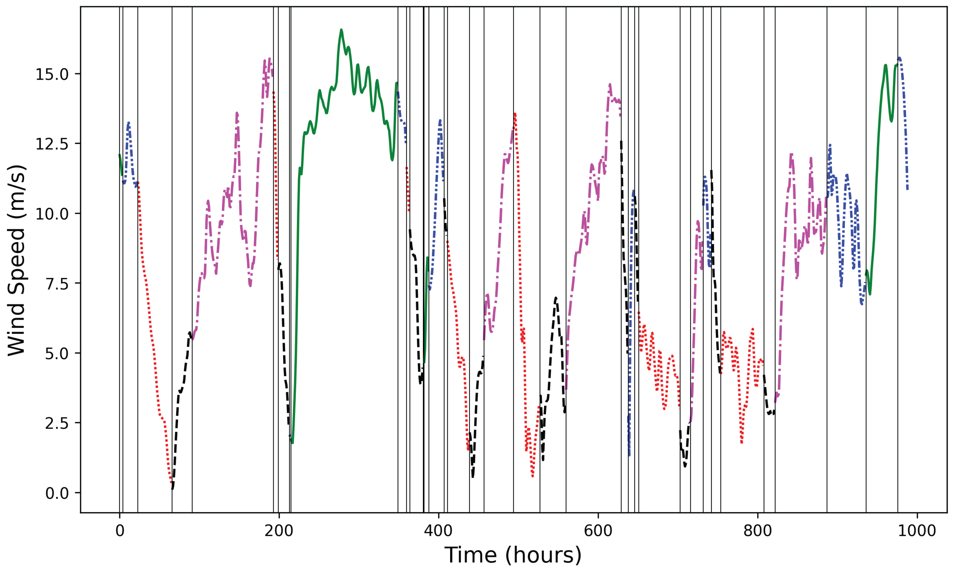
Figure 1 presents the wind-speed time series clustering with the Dirichlet process for the last 1000 h of one of our data sets. In Figure 1, each line style represents a different cluster type, and vertical lines form the clustering blocks. In this data set, the DP model results in five clusters.

3.2. Dynamic Time Warping

Dynamic time warping (DTW) is a widely used similarity measurement for time series. DTW enables to explore data points that have similar shapes at the different parts of the time series data [36].
Suppose X = ( x 1 , x 2 , , x N ) , Y = ( y 1 , y 2 , , y M ) denote two different time series where x i is ith point in X and y j is jth point in Y, and N and M are size of the X and Y, respectively. Let d ( x i , y j ) be distance between data points of x i and y j and A M N matrix where a i , j = d ( x i , y j ) . A warping path is a set of adjacent matrix elements of A M × N [37]. A warping path P is defined as P = { p 1 , p 2 , , p t , , p K } , f o r max { M , N } < K M + N 1 . The DTW is calculated as follows:
D T W ( X , Y ) = D ( M , N ) = min P t = 1 K d ( i t , j t )
where D is the accumulated distance matrix. The DTW distance is the minimum distance between time series of X and Y. The best warping path in accumulated distance matrix D(M,N) can be calculated as follows:
D ( i , j ) = d ( i , j ) + min D ( i , j 1 ) D ( i 1 , j 1 ) D ( i 1 , j )
Figure 2 presents the wind-speed time series clustering with dynamic time warping for the last 1000 h of one of our data sets. As in Section 3.1, in Figure 2, each line style represents a different type of cluster, and vertical lines form the clustering blocks. In dynamic time warping, the number of clusters is predetermined as five.

3.3. Long Short-Term Memory (LSTM)

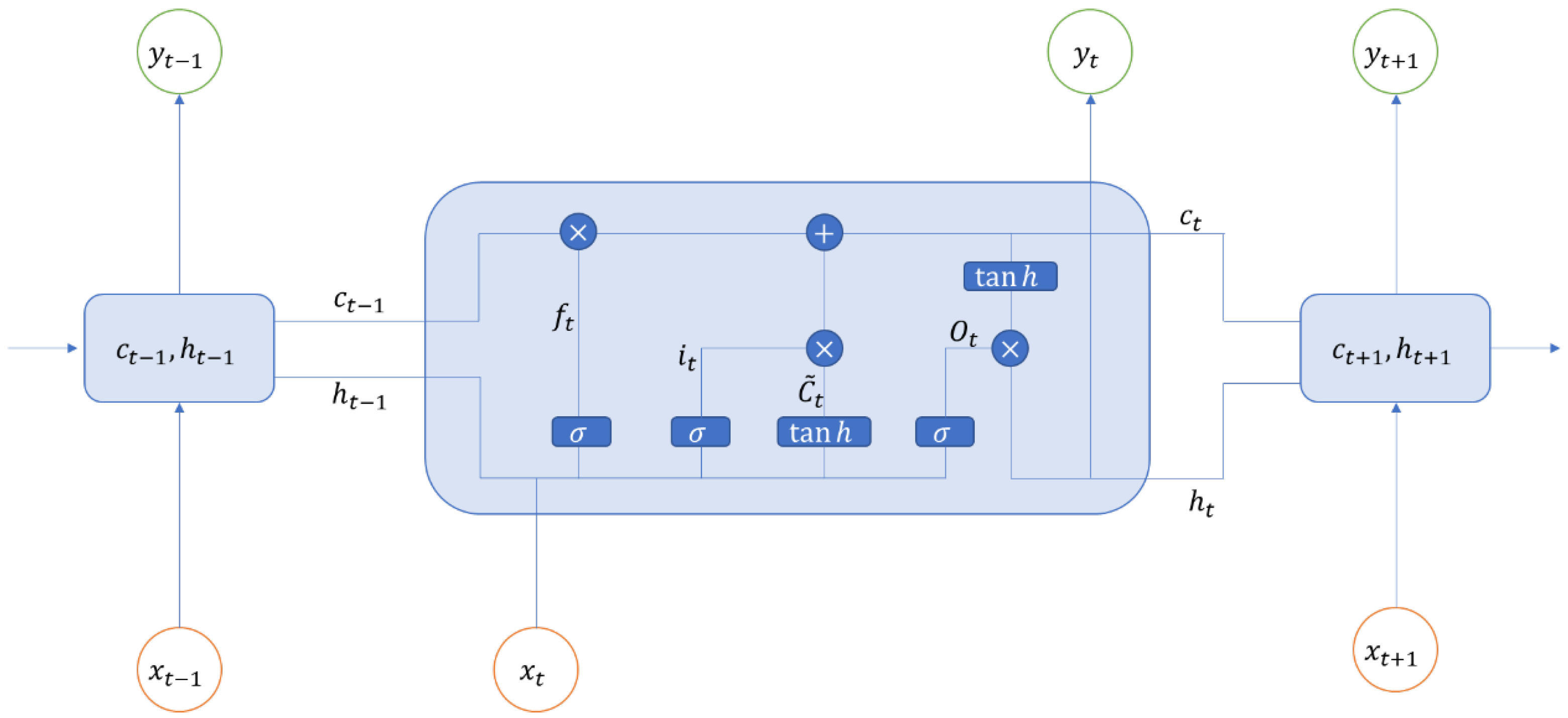
LSTM network is an ANN architecture that is developed to tackle the vanishing gradients problem [38]. LSTM preserves useful information about previous data in the sequence and propagates into the network if needed. In order to restrain the vanishing gradients problem, LSTM utilizes forget gates to retain useful data. The design of the LSTM cell is visualized in Figure 3.
LSTMs use a set of “gates” (forget, input and output) to control how a sequence of data enters to the network, is stored, and leaves the network. The forgetting gate determines which data are useful given both input ( X t ) and the previous hidden layer ( h t 1 ) data. At the forget gate, a sigmoid activation function (given in Equation (6)) is used to generate a vector where each element is within [0, 1].
f t = σ ( W f , x X t + W f , h h t 1 + b f )
The input gate first determines which data will be stored in long-term memory given both input ( X t ) and previous hidden layer ( h t 1 ) data. At this process, t a n h activation function (Equation (7)) is used to combine input and the previous hidden layer data and obtain candidate data ( C ˜ ). Then, which components of the candidate data are worth keeping is determined by using sigmoid activation function (Equation (8)). Finally, new long-term memory is obtained as in Equation (9).
C t ˜ = t a n h ( W c , x X t + W c , h h t 1 + b c )
i t = σ ( W i , x X t + W i , h h t 1 + b i )
C t = C t 1 f t + i t C t ˜
The output gate decides output data ( o t ) (Equation (10)) and new hidden layer (Equation (11)) given the previous hidden layer and new input data.
o t = σ ( W o , x X t + W o , h h t 1 + b o )
h t = o t t a n h ( C t )

4. Proposed Model

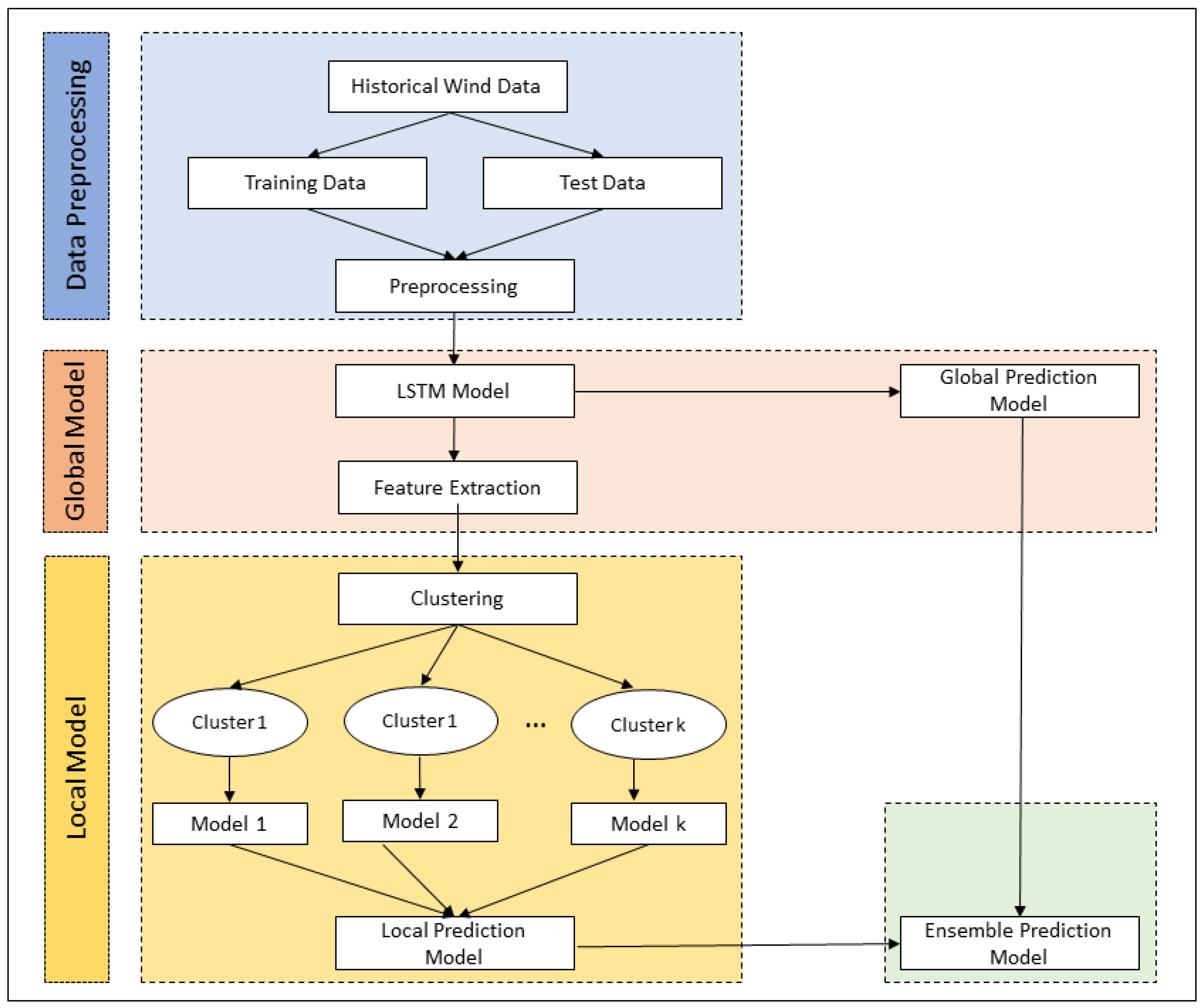
Most of the existing forecasting models in wind speed use the whole historic data in prediction, which are subject to be affected by seasonality. This study proposes a wind speed forecasting model for short-term based on the Dirichlet mixture model, dynamic time warping, and deep learning containing three stages. Figure 4 presents the flowchart of the proposed model.
In the first stage, an LSTM deep learning model is constructed using whole data, which is referred to as the global model in the rest of the paper. The output of the trained LSTM layer is used for features that represent the temporal relationship of the time-series data. In the second stage, a Dirichlet mixture model and dynamic time-warping approaches are applied to features that are extracted at LSTM layer separately to cluster time series data. In the clustering process, the number of clusters is determined by Dirichlet mixture modeling.
In the third stage, an LSTM deep learning model (local model) is created for each cluster. Particularly, constructing deep learning models using clustered data will reveal local patterns, while global models reveal global patterns. In the prediction stage, features of the test data are extracted from the LSTM layer of the global model. Thereafter, the test data are assigned to the corresponding cluster using the applied clustering model. Finally, the forecast is made by utilizing the assigned cluster’s local LSTM model.
We also construct an ensemble model which exploits the advantages of both the global and local LSTM models. In this model, both local and global LSTM models are ensembled as depicted in Figure 4.

5. Experiment Design and Results

This section first briefly explains the data sets’ attributes and performance metrics. Then, the described data sets are utilized to assess the introduced models’ capability. Finally, the proposed models’ results are analyzed and compared with the benchmark model.

5.1. Data Sets Description

This study uses four data sets to validate the proposed forecasting method. These four data sets are obtained from four different regions of Turkey (Cesme-Izmir, Amasra-Bartin and Pirbasi-Kayseri, and Gokceada-Canakkale). The selected locations are located in different parts of Turkey with different climates and wind regimes. The selected locations are shown in Figure 5.
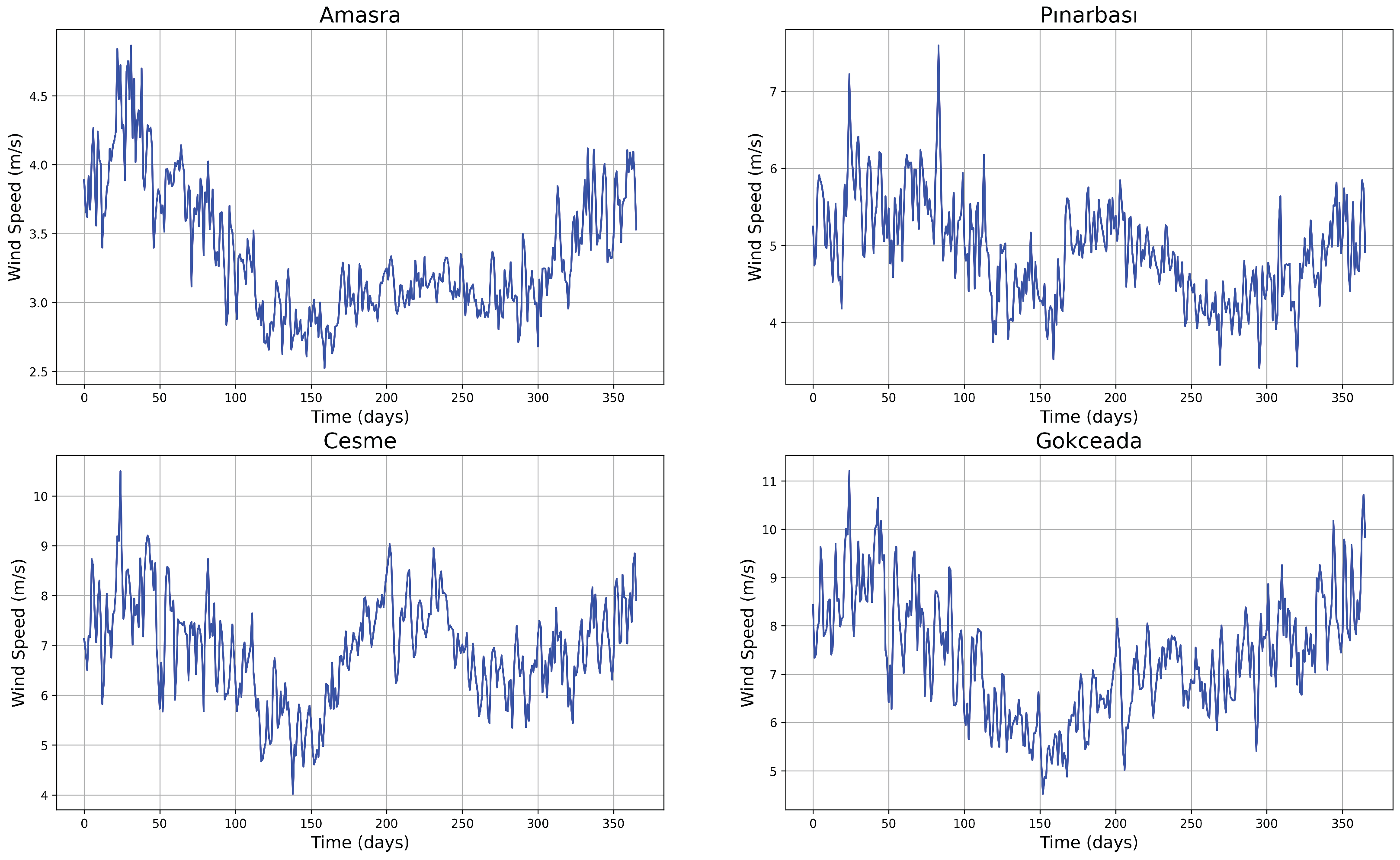
The four data sets are hourly data points from 1 January 2001 to 31 March 2021. Each data set contains hourly wind speed, surface pressure, wind direction, humidity, and temperature values. The data is divided into two subgroups training and testing. The training and testing data contain 80 % and 20 % of the whole data set, respectively. In order to show wind speed characteristics of the selected locations, Figure 6 depicts the daily averages of wind speed. As shown in Figure 6, different wind regimes and daily wind averages.

5.2. Performance Metrics

We use three different evaluation metrics to validate the proposed forecasting model. Mean absolute error (MAE) measures the difference between two observed and predicted values, mean absolute percentage error (MAPE) evaluates the mean of absolute percentage errors of prediction, and root mean square error (RMSE) measures the standard deviation of forecasting errors. The employed performance metrics are given in Table 1.

5.3. Numerical Results and Analysis

The data for selected locations is standardized by subtracting by mean and dividing by standard deviation and used as input in the proposed models. The input variables are historical wind speed, surface pressure, wind direction, humidity and temperature values, and the output variable is the forecasted wind speed an hour ahead time horizon. The performance of the global LSTM, the Dirichlet process local LSTM (DP-local LSTM), the dynamic time warping local LSTM (DTW-local LSTM), Dirichlet process ensemble model (DP-ensemble), and dynamic time warping ensemble model (DTW-ensemble) are compared using MAE, MPAE, and RMSE metrics. The performance of each method for each location is given in Table 2. As depicted in Table 2, the ensemble models’ performance is the best among all the compared models regardless of evaluation metrics, clustering approach, and locations. For most of the cases (amasra, pinarbasi, and cesme), the DP-local LSTM model is superior to global LSTM and DTW-local LSTM. This result may probably arise due to consistent wind speed. Table 2 also shows that the DP-ensemble model is superior to the DTW-ensemble model, which implies that the clustering approach is also important in wind-speed forecasting.
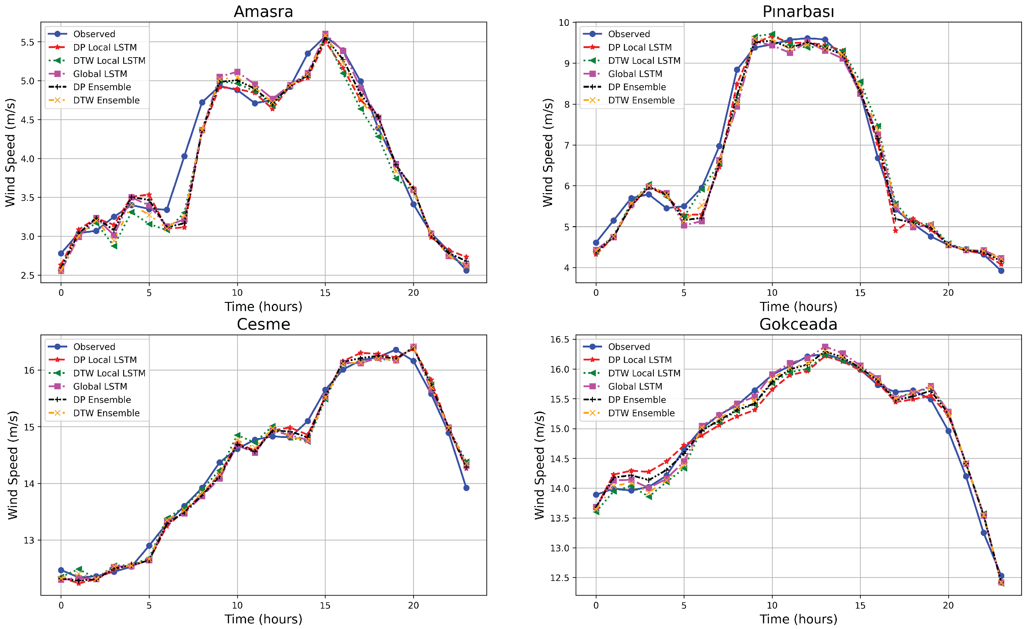
Figure 7 shows each method’s actual wind speed values and forecast values. While all methods achieve relatively good performance, the ensemble model achieves the best performance in all data sets.

6. Conclusions and Future Work

The accuracy of wind speed forecasting is crucial for the reliability of wind energy. In this work, we study a Bayesian clustering-based deep learning model for short-term wind speed forecasting to improve the prediction accuracy. The proposed model takes advantage of clustering the features obtained from the LSTM layer. Features extracted from the LSTM layer will reveal the temporal relationship of the time series data, which will make the segmentation of the time series more accurate. Particularly, Dirichlet mixture modeling and dynamic time warping methods are applied to features extracted at the LSTM layer to cluster time series data to focus on short-term patterns. The ensemble model captures both long and short-term patterns integrating global and local models.
The numerical study with four different data shows that the proposed ensemble model improves the prediction accuracy based on three evaluation metrics (MAE, MAPE, RMSE). Our results also show that all of the methods studied achieve relatively good performance in wind forecasting. The ensemble models’ prediction accuracy are the best among studied methods regardless of the wind regime and meteorological aspects (for all locations). Our results indicate that the proposed models will improve wind energy investments’ reliability and economic success. The numerical results also reveal that clustering approaches have critical roles in prediction accuracy.
The proposed deep learning model is trained on large data (with 141,984 data points), which is computationally demanding. In future work, instead of training the whole model, transfer learning method can be used to extract features. In particular, features could be obtained from a pretrained model, and train only the last layer to save substantial computational resources. It might also be worthwhile to use different nonparametric methods for clustering features. Models with different data types from different areas (such as marketing and supply chain management) might be another important extension. Another possible extension of this study would be utilizing different machine learning algorithms to the proposed approach.

Funding

This research received no external funding.

Conflicts of Interest

The author declares no conflict of interest.

References

  1. Global Wind Energy Council. GWEC|Global Wind Report 2021; Global Wind Energy Council: Brussels, Belgium, 2021. [Google Scholar]
  2. Chen, G.; Tang, B.; Zeng, X.; Zhou, P.; Kang, P.; Long, H. Short-term wind speed forecasting based on long short-term memory and improved BP neural network. Int. J. Electr. Power Energy Syst. 2022, 134, 107365. [Google Scholar] [CrossRef]
  3. Albalawi, H.; El-Shimy, M.E.; AbdelMeguid, H.; Kassem, A.M.; Zaid, S.A. Analysis of a Hybrid Wind/Photovoltaic Energy System Controlled by Brain Emotional Learning-Based Intelligent Controller. Sustainability 2022, 14, 4775. [Google Scholar] [CrossRef]
  4. Zeng, P.; Sun, X.; Farnham, D.J. Skillful statistical models to predict seasonal wind speed and solar radiation in a Yangtze River estuary case study. Sci. Rep. 2020, 10, 8597. [Google Scholar] [CrossRef] [PubMed]
  5. Shang, Z.; He, Z.; Chen, Y.; Chen, Y.; Xu, M. Short-term wind speed forecasting system based on multivariate time series and multi-objective optimization. Energy 2022, 238, 122024. [Google Scholar] [CrossRef]
  6. Carvalho, D.; Rocha, A.; Gómez-Gesteira, M.; Santos, C. A sensitivity study of the WRF model in wind simulation for an area of high wind energy. Environ. Model. Softw. 2012, 33, 23–34. [Google Scholar] [CrossRef] [Green Version]
  7. Fang, S.; Chiang, H.D. Improving supervised wind power forecasting models using extended numerical weather variables and unlabelled data. IET Renew. Power Gener. 2016, 10, 1616–1624. [Google Scholar] [CrossRef]
  8. Sun, F.; Jin, T. A hybrid approach to multi-step, short-term wind speed forecasting using correlated features. Renewable Energy 2022, 186, 742–754. [Google Scholar] [CrossRef]
  9. Demolli, H.; Dokuz, A.S.; Ecemis, A.; Gokcek, M. Wind power forecasting based on daily wind speed data using machine learning algorithms. Energy Convers. Manag. 2019, 198, 111823. [Google Scholar] [CrossRef]
  10. Hoolohan, V.; Tomlin, A.S.; Cockerill, T. Improved near surface wind speed predictions using Gaussian process regression combined with numerical weather predictions and observed meteorological data. Renew. Energy 2018, 126, 1043–1054. [Google Scholar] [CrossRef]
  11. Brown, B.G.; Katz, R.W.; Murphy, A.H. Time series models to simulate and forecast wind speed and wind power. J. Appl. Meteorol. Climatol. 1984, 23, 1184–1195. [Google Scholar] [CrossRef]
  12. Torres, J.; García, A.; De Blas, M.; De Francisco, A. Forecast of hourly average wind speed with ARMA models in Navarre (Spain). Sol. Energy 2005, 79, 65–77. [Google Scholar] [CrossRef]
  13. Rajagopalan, S.; Santoso, S. Wind power forecasting and error analysis using the autoregressive moving average modeling. In Proceedings of the 2009 IEEE Power Energy Society General Meeting, Calgary, AB, Canada, 26–30 July 2009; pp. 1–6. [Google Scholar]
  14. Sfetsos, A. A novel approach for the forecasting of mean hourly wind speed time series. Renew. Energy 2002, 27, 163–174. [Google Scholar] [CrossRef]
  15. Kavasseri, R.G.; Seetharaman, K. Day-ahead wind speed forecasting using f-ARIMA models. Renew. Energy 2009, 34, 1388–1393. [Google Scholar] [CrossRef]
  16. Eldali, F.A.; Hansen, T.M.; Suryanarayanan, S.; Chong, E.K.P. Employing ARIMA models to improve wind power forecasts: A case study in ERCOT. In Proceedings of the 2016 North American Power Symposium (NAPS), Denver, CO, USA, 18–20 September 2016; pp. 1–6. [Google Scholar]
  17. Dokuz, A.; Demolli, H.; Gokcek, M.; Ecemis, A. Year-ahead wind speed forecasting using a clustering-statistical hybrid method. In Proceedings of the CIEA’2018 International Conference on Innovative Engineering Applications, Sivas, Turkey, 20–22 September 2018; pp. 971–975. [Google Scholar]
  18. Liu, X.; Lin, Z.; Feng, Z. Short-term offshore wind speed forecast by seasonal ARIMA—A comparison against GRU and LSTM. Energy 2021, 227, 120492. [Google Scholar] [CrossRef]
  19. Cadenas, E.; Rivera, W.; Campos-Amezcua, R.; Heard, C. Wind Speed Prediction Using a Univariate ARIMA Model and a Multivariate NARX Model. Energies 2016, 9, 109. [Google Scholar] [CrossRef] [Green Version]
  20. Cadenas, E.; Rivera, W. Short term wind speed forecasting in La Venta, Oaxaca, México, using artificial neural networks. Renew. Energy 2009, 34, 274–278. [Google Scholar] [CrossRef]
  21. Dumitru, C.D.; Gligor, A. Daily Average Wind Energy Forecasting Using Artificial Neural Networks. Procedia Eng. 2017, 181, 829–836. [Google Scholar] [CrossRef]
  22. Higashiyama, K.; Fujimoto, Y.; Hayashi, Y. Feature extraction of numerical weather prediction results toward reliable wind power prediction. In Proceedings of the 2017 IEEE PES Innovative Smart Grid Technologies Conference Europe (ISGT-Europe), Turin, Italy, 26–29 September 2017; pp. 1–6. [Google Scholar]
  23. Yu, R.; Liu, Z.; Li, X.; Lu, W.; Ma, D.; Yu, M.; Wang, J.; Li, B. Scene learning: Deep convolutional networks for wind power prediction by embedding turbines into grid space. Appl. Energy 2019, 238, 249–257. [Google Scholar] [CrossRef] [Green Version]
  24. Shabbir, N.; Kütt, L.; Jawad, M.; Husev, O.; Rehman, A.U.; Gardezi, A.A.; Shafiq, M.; Choi, J.G. Short-Term Wind Energy Forecasting Using Deep Learning-Based Predictive Analytics. Comput. Mater. Contin. 2022, 72, 1017–1033. [Google Scholar] [CrossRef]
  25. Li, C.; Lin, S.; Xu, F.; Liu, D.; Liu, J. Short-term wind power prediction based on data mining technology and improved support vector machine method: A case study in Northwest China. J. Clean. Prod. 2018, 205, 909–922. [Google Scholar] [CrossRef]
  26. Liu, H.; Mi, X.; Li, Y. Smart deep learning based wind speed prediction model using wavelet packet decomposition, convolutional neural network and convolutional long short term memory network. Energy Convers. Manag. 2018, 166, 120–131. [Google Scholar] [CrossRef]
  27. López, G.; Arboleya, P. Short-term wind speed forecasting over complex terrain using linear regression models and multivariable LSTM and NARX networks in the Andes Mountains, Ecuador. Renew. Energy 2022, 183, 351–368. [Google Scholar] [CrossRef]
  28. Xiong, B.; Lou, L.; Meng, X.; Wang, X.; Ma, H.; Wang, Z. Short-term wind power forecasting based on Attention Mechanism and Deep Learning. Electr. Power Syst. Res. 2022, 206, 107776. [Google Scholar] [CrossRef]
  29. Yu, C.; Li, Y.; Bao, Y.; Tang, H.; Zhai, G. A novel framework for wind speed prediction based on recurrent neural networks and support vector machine. Energy Convers. Manag. 2018, 178, 137–145. [Google Scholar] [CrossRef]
  30. Praveena, R.; Dhanalakshmi, K. Wind Power Forecasting in Short-Term using Fuzzy K-Means Clustering and Neural Network. In Proceedings of the 2018 International Conference on Intelligent Computing and Communication for Smart World (I2C2SW), Erode, India, 14–15 December 2018; pp. 336–339. [Google Scholar]
  31. Kim, S.; Tadesse, M.G.; Vannucci, M. Variable selection in clustering via Dirichlet process mixture models. Biometrika 2006, 93, 877–893. [Google Scholar] [CrossRef] [Green Version]
  32. Ferguson, T.S. A Bayesian analysis of some nonparametric problems. Ann. Stat. 1973, 1, 209–230. [Google Scholar] [CrossRef]
  33. Chen, J.; Gong, Z.; Liu, W. A Dirichlet process biterm-based mixture model for short text stream clustering. Appl. Intell. 2020, 50, 1609–1619. [Google Scholar] [CrossRef]
  34. Escobar, M.D.; West, M. Bayesian density estimation and inference using mixtures. J. Am. Stat. Assoc. 1995, 90, 577–588. [Google Scholar] [CrossRef]
  35. Li, Y.; Schofield, E.; Gönen, M. A tutorial on Dirichlet process mixture modeling. J. Math. Psychol. 2019, 91, 128–144. [Google Scholar] [CrossRef]
  36. Li, H. Time works well: Dynamic time warping based on time weighting for time series data mining. Inf. Sci. 2021, 547, 592–608. [Google Scholar] [CrossRef]
  37. Li, H.; Liu, J.; Yang, Z.; Liu, R.W.; Wu, K.; Wan, Y. Adaptively constrained dynamic time warping for time series classification and clustering. Inf. Sci. 2020, 534, 97–116. [Google Scholar] [CrossRef]
  38. Hochreiter, S.; Schmidhuber, J. Long short-term memory. Neural Comput. 1997, 9, 1735–1780. [Google Scholar] [CrossRef] [PubMed]
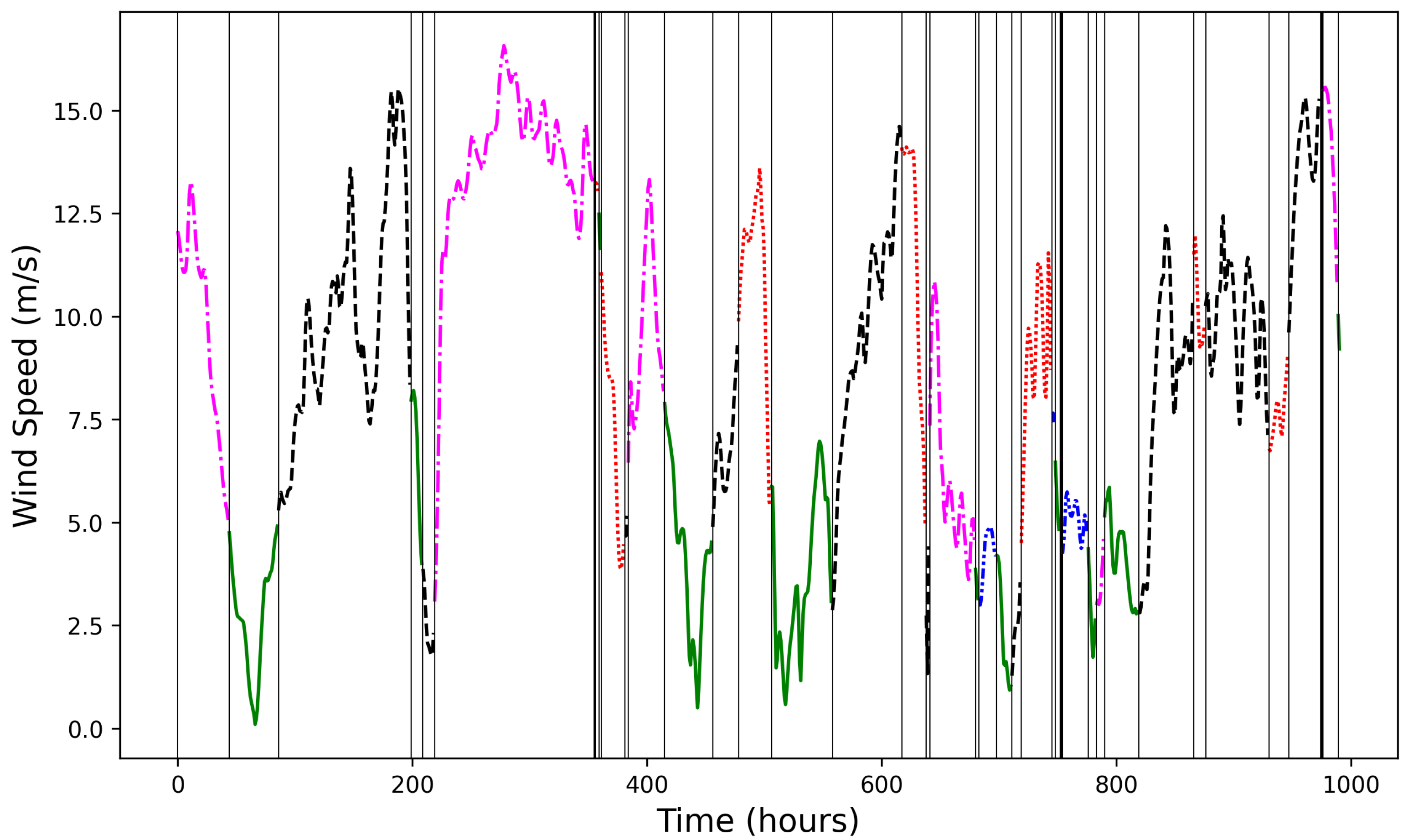
Figure 1. The Dirichlet process clustering.
Applsci 12 13031 g001
Figure 2. The dynamic time warping clustering.
Applsci 12 13031 g002
Figure 3. The LSTM architecture.
Applsci 12 13031 g003
Figure 4. The flowchart of the proposed forecasting model.
Applsci 12 13031 g004
Figure 5. The data sets obtained locations.
Applsci 12 13031 g005
Figure 6. Daily averages of wind speed at selected locations.
Applsci 12 13031 g006
Figure 7. Actual and forecasted wind speed values for each method for 24 h time horizon.
Applsci 12 13031 g007
Table 1. Performance metrics.
MetricsDefinition
MAE 1 N j = 1 n | y j y ^ j |
MAPE 100 N j = 1 n | y j y ^ j | | y j |
RMSE 1 N j = 1 n ( y j y ^ j ) 2
y j : Observed value and y ^ j : forecasted value.
Table 2. The performance of each method for a different test location.
AmasraPinarbasiCesmeGokceada
Models-MetricsMAEMAPERMSEMAEMAPERMSEMAEMAPERMSEMAEMAPERMSE
Golabal LSTM0.1868.6860.2690.2316.9590.3580.1724.4200.2600.1974.5900.311
DP-Local LSTM0.1858.6070.2730.2256.4990.3540.1664.1200.2600.1994.9570.326
DTW-Local LSTM0.1938.8010.2830.2376.8890.3660.1694.0850.2620.1964.5960.325
DP-ensemble model0.1758.2660.2580.2176.4170.3430.1614.0900.2500.1864.5390.304
DTW-ensemble model0.1798.3470.2620.2226.5640.3470.1644.1140.2530.1874.4180.305
Publisher’s Note: MDPI stays neutral with regard to jurisdictional claims in published maps and institutional affiliations.