Analysis of Factors Influencing the Prices of Tourist Offers

Abstract

Tourism is a significant branch of many world economies. Many factors influence the volume of tourist traffic and the prices of trips. There are factors that clearly affect tourism, such as COVID-19. The paper describes the methods of machine learning and process mining that allow for assessing the impact of various factors (micro, mezzo and macro) on the prices of tourist offers. The methods were used on large sets of real data from two tour operators, and the results of these studies are discussed in this paper. The research presented is part of a larger project aiming at predicting trip prices. It answers the question of which factors have the greatest impact on the price and which can be omitted in further work. Nevertheless, the dynamic world situation suggests that the ranking of factors may change and the presented universal methods may provide different results in the coming years.

1. Introduction

The paper reports on the part of a research project under the ePredyktour project, which is an attempt to solve a problem of predicting trip prices on the basis of various factors. The presented research was carried out for data provided by two Polish tour operators in 2021. In Poland, expenditure on tourism and recreation in the consumption basket amounted to 8.2% (in 2018). Poles more often choose organized trips than trips on their own. They account for 1.6% of the consumption basket compared to 1% in the European Union. The COVID-19 pandemic had a heavy impact on the travel industry. In most countries, the contribution of tourism to GDP has decreased significantly; in Poland, this decrease amounted to about 2 percentage points in total GDP [1]. Therefore, in 2021, the COVID pandemic is the overarching factor influencing the tourism industry, and certainly has an impact on the conclusions drawn from the presented research. Nevertheless, the methods proposed in the paper are universal and can be repeated for data before and after the pandemic.

The entire ePredyktour project consists of the following stages (presented in Figure 1):

Stage I:

Theoretical analysis and definition of various factors that may affect the price of the trip, finding the sources of these factors and performing initial normalization. This stage was made by specialists in the tourism industry. At this stage, it turned out that it is not possible to access all the databases that were theoretically considered. For example, various opinions posted on social media could not be used in this project due to a lack of authorization. The identified factors have been divided into three groups: micro (factors directly related to a given trip, such as hotel properties, transport type, type of meals, etc.), mezzo (factors related to the vicinity of the holiday destination, such as weather, historic attraction, terrorist attacks risk, etc.), and macro (global factors such as fuel prices, exchange rates, economic indicators, etc.)

Stage II:

The raw data from the various databases were downloaded, transformed into predefined structures and saved on the Hadoop Distributed File System (HDFS) [2]. These data are available in the form of Data Frames via the API of the Apache Spark [3]. The tourism, IT and big data specialists were responsible for this stage. Data were collected from the beginning of 2021 and initially collections were created for two tour operators. Each trip was recorded almost daily to a new record. In this way, millions of records were created.

Stage III:

This stage is the subject of the paper and the authors were responsible for its implementation. Its goal was the analysis of factors in order to determine their impact on both the entry price and the change in the price of trips. The latter task was of particular importance, as the whole project aims to design a system that predicts changes in trip prices. Initially, the data were transformed into structures corresponding to the input of the machine learning algorithms and several algorithms were used to evaluate the influence of various factors on the changes of trip prices. Theses methods and the results achieved are the subject of the following sections of this paper.

Stage IV:

The use of machine learning algorithms, which, based on the factors examined in Stage III, will predict the price of the trip currently offered by the tour operator. During the preparation of this paper, this stage was still in progress.

As a result of Stage II, six datasets have been created: offers, trips, properties, nbp, opec, and tradingeconomics. When a client comes to a travel agency, he/she first chooses an offer, whose name in the case of stays is the same as the name of the hotel (eg. Hotel Sea), and, in the case of touring trips, it is related to the scope of the trip (e.g., the most beautiful towns of Provence). This information is included in the offers set. Then, the details of the trip are selected: day of departure and return, transport and food type, standard of the room, number of persons, etc. These details are included in the trips dataset. The properties set provides general information about hotels. The sets: nbp (dollar, euro, and pound exchange rates), opec (oil barrel price), and tradingeconomics (consumer spending, GDP per capita, inflation rate, personal savings, and unemployment rate) represent the macro factors. The price applies to each trip and it depend on numerous factors; it is set at the presentation time and may change over time.

All factors considered in the project can be divided into constant and changing over time within a given trip. This division is important for the analysis, because the constant factors play a different role than the changing ones. The constant factors are the basis for setting initial prices of trips and grouping trips according to certain features. On the other hand, the changing factors have a hypothetical greater impact on the change of the price of a given trip over time; hence, they may be more useful for price prediction. All these factors, divided into constant and time varying are described in Section 3.

It is worth mentioning that not all of these factors change with the same frequency. The barrel price and exchange rates change daily, but economic indicators rarely change: once a month, once every six months, or even once a year. The current weather may also change every day, while the forecast weather on the day of departure does not start to change until two weeks before departure due to the reliability of weather forecasts. The aim of this research it to evaluate which of all these factors, both constant and time-varying ones, are worth being considered while analyzing the dynamics of trip prices. The factors identified as having significant influence on trip prices will be used to create a price prediction model in stage IV of the project. A tool created in this way might be implemented in a meta-search engine of trips and offered as Software, or as a Service, useful from the point of view of tour operators, travel agents, or hotel owners. The market demand for the project results has been confirmed by potential recipients of the system.

The rest of the paper is organized as follows. Section 2 presents other studies on predicting some parameters related to tourism, e.g., tourism demand or tourists’ satisfaction. It also mentions methods applied in other areas but that are potentially adequate in this application. Section 3 of the paper presents a feature selection approach applied to evaluate the predictive power of individual trip attributes to the changes of prices. These methods belong to the category of feature engineering and are commonly implemented in machine learning systems. They not only enable one to evaluate the features independently, but also to identify subsets of these parameters optimal for a given task. Section 4 outlines a different approach to the problem at hand: creating and analyzing a model of the price change process. For this purpose, various tools and algorithms for process mining [4] were used. This approach allows one to look at the price change process in the context of changing other factors and to find other interesting relationships. Section 5 presents conclusions drawn on the basis of the obtained results and some ideas for future works.

2. Related Work

To select all the factors that influence the price of a trip, enormous data from around the world would have to be analyzed. This is because tourism covers almost the entire world and is available to people of various affluence level, views, culture, style of recreation, preferred climate, etc. Of course, such calculations are practically impossible. In this project, a set of factors identified by a team of tourism experts and technically feasible were used (see Table 1).

There are papers in the literature that also select certain factors in order to automatically analyze their impact on tourism. A variable often treated as a target is tourism demand. In [5], the first challenge in the research was also to determine the set of factors influencing tourism in order to forecast the tourism demand. Initially, the factors were divided into three categories: the first contained tourist origin, the economic level, and the personal situation of tourists, the second was related to the supply of tourist destinations, including the attraction, price, infrastructure, and travel organization, the third contained consumer price comparison, promotion, exchange rate, policy coordination, and socio-economic and cultural heterogeneity. As a result, seven factors were selected that allowed one to create a feature vector. These are: number of inbound tourists, currency exchange rate, per capita GDP, total import and export of goods, population, per capita GDP of destination countries, and virtual variables, that can reflect the situation of special events and improve the prediction model. The vector is then used in the neural network algorithm to forecast the inbound tourism demand.

Demand function forecasting is also the subject of [6], where authors consider a panel of over 100 hotels in Milan (Italy), over a time interval of 274 days to determine the demand function for these hotels. The price index was a leading indicator in the set of explanatory variables. In economic theory, with other factors being constant, demand is inversely proportional to price. The close relationship between price and demand may suggest that other factors influencing demand may also influence price. The authors took into account the following factors related mainly to the properties of the hotel and its surroundings: occupation rate, number of rooms, meeting rooms, restaurant seats, distance from city center, distance fom from airport, holidays, and events. Most of these determinants were also taken into account in the discussed project. It is worth noting that, apart from the price and occupation rate, the rest of these factors are constant. Using the collected data, the authors proposed a method of forecasting tourist demand by improving the set of available information.

Another topic of research that takes into account tourism determinants are travel recommendation systems. From the point of view of tour operators, data collected by such a system allows for the study of customer preferences, and thus for price regulation. It is therefore important what factors customers consider as they may affect the price of the trip. In [7], the authors have listed a set of factors that are used to investigate customer preferences. Some of them are global, such as weather, season, weekday, transport, crowdedness and distance, while others are related to specific client preferences, such as budget, companion, feeling, travel goal and knowledge of the travel area. For many customers, the weather is the primary factor in choosing trips, especially leisure ones. However, “good weather” can mean different things for different people and different locations. It can be assumed that customers going to Greece, Italy or Croatia in the summer count on a lot of sunny days, warm water and accept the heat, while visitors to Iceland or Norway expect a few days without rain and skiers expect snow. In paper [8], the authors examined various weather factors for point of interest recommendations. They took into account the following factors: visibility, precipitation intensity, humidity, cloud cover, pressure, wind speed, temperature, and moon phase. The conducted research confirmed that the influence of factors differs depending on the location. For example, in Honolulu, the best performing feature is precipitation intensity, while in Minneapolis it is visibility. Likewise, the phases of the moon, which generally have little influence on the choice of destination, are crucial in certain specific places.

In most publications on tourism, price is a factor (or one of the factors) for determining or forecasting other values related to tourism, e.g., a demand mentioned above. However, in [9], the author presents research on the price effects of demand and the results of interviews with tourists. Three variables were identified and used as factors in this study: airfare, hotel tariffs, and the exchange rate. However, this paper was published in 1994, and since then there have been many changes in tourism itself, as well as in information technology, data size, access to various offers, and tourists’ expectations.

There are applications that can predict the prices of certain components of trips. Most of the time, it concerns searching for flights with the history of prices and information about the forecast price in the future. Google Flights [10] and Momondo [11] are examples of such search engines.

The most straightforward approach to the problem of finding good predictors is feature selection. It is a process of reducing the number of original attributes to a subset good enough to predict the value of a target variable. There are some examples of applying feature selection methods in tourism. In [12], for example, the authors managed to select a number of keywords extracted from web search data to predict monthly statistics of China inbound foreign visitors. They applied random forest to estimate the importance of individual features, which were keyword frequencies. A similar idea of selecting keywords has been proposed in [13] in order to forecast tourist demand and hotel occupancy from search query data. In this case, the features were filtered in various ways, i.e., on the basis of correlation coefficient, information gain or random forest importance, by running the recursive elimination or genetic algorithm. Removing redundant and extraneous information enabled us to improve the forecasting accuracy.

Tourist reviews deliver lots of valuable data, which can be used to infer tourists’ satisfaction, as for example in [14], where reviews of tourist agencies were analyzed. A number of keywords used as features were processed. The performed feature selection based on LASSO regression model revealed top factors affecting the satisfaction. The interesting fact was the discovery of several new factors that became essential after COVID-19, i.e., refunds, bad reviews, assurance, and comparison. Satisfaction predictors were also analysed in [15], where results obtained by a feature selection filter were used as weights for traditional tf-idf feature values. This leads to the improvement of performance of sentiment analysis of online reviews of tourist attractions.

Another interesting application of feature selection has been presented in [16]. In this study, several methods were implemented to find sets of features good for the classification of Polish voivodeships according to their tourist attractiveness. One of the main conclusions of this paper was that different selection methods lead to significant differences in classification results.

To estimate the influence of selected variables on prices regression, models trained to predict prices are often implemented. Although there are a lot of studies on predicting prices of various products, there are no studies on predicting the prices of trip packages. However, the regression approach is worth taking into account. In [17], the regression approach has been applied to predict the prices of a set of products sold online. The authors implemented classical linear regression and least squares SVM with an artificial bee colony to optimize its parameters. The latter method let us achieve higher prediction accuracy. The method was implemented in a web application both to alert users when the price of a product changed and to predict the price for the next day. It might be useful for customers, as it enables monitoring product pricing.

House prices have always been of particular interest. In [18], the authors analyzed a number of papers on significant factors influencing house prices. Among various determinants grouped into locational, structural, and neighbourhood, the locational ones turned out to be the most significant in fixing the prices of houses. Various methods were applied to create models able to predict prices of houses, e.g., support vector regression, neural networks, and gradient boosting. The hedonic model, which applies multivariate regression analysis, is the simplest way to estimate the significance of various factors. The obtained regression coefficients may be treated as factor weights indicating their influence on the target variable [19]. Interesting findings were presented in [20]. It has been demonstrated that partitioning the data on the basis of selected factors and applying a multi-task learning algorithm may improve the performance of house price prediction.

There are also some research studies where dynamic factor approach, which is a tool commonly used for analyzing economic data, is applied in forecasting some tourism indices. Classical dynamic factor models represent the whole cross-section dynamics by a few common factors found, for example, by PCA and then perform forecasting for a target variable on the basis of these common factors using a simple linear regression model. It has been applied, for example, in [21] to predict checking-in and overnight stays of travellers in Spain on the basis of the numbers of queries on several traveling related topics. The authors managed to obtain good results for short-term forecasts. To relax the limitation of the classical dynamic factor model, which does not allow for correlations between idiosyncratic components, a generalised dynamic factor model (GDFM) [22] was proposed. This model was applied by the authors of [23]. They created a time-varying parameter factor vector autoregressive model based on GDFM to analyze the influence of six factors (dining, transportation, attractions, shopping, tours, and lodging) on tourist demand in different periods of time. The model investigated the time-varying characteristics of the relationship between variables. The original six factors were extracted from search queries and represented by selected keyword frequencies. They found that tourism demand responded more intensely to shock in dining, tours, and lodging than to the other three factors. Dining, attractions, and shopping had a positive effect on tourism demand, whereas transportation, tours, and lodging had negative effect. The presented analysis is rather unique, as it is a simultaneous quantitative analysis of several factors.

As already mentioned in the Introduction, time varying factors (see Table 1), as well as the price of the trip itself, change over time. Any change to the trip price can be treated as an event in the price change process. This event may be the consequence or cause of other events. This allows for the use of business process models to implement the price change process. The authors of [24] presented the process model in the form of Colored Petri Net (CPN) for determining activities related to changes in the prices of stocks. They analyzed trends of change, rather than changes in individual prices, as the prices of stocks fluctuate on almost every stock quote. Trends influence decisions to buy, sell, or hold stocks, and the presented CPN helps users make that decision. The model is predefined and immutable. Price changes at tour operators occur much less frequently, often without clear trends, so each increase or decrease can be analyzed. The use of process mining to automatically determine price change processes is a new application of these techniques.

This paper presents an idea of applying several feature selection methods and the process mining technique to evaluate the influence of various factors on the changes of trip prices. The novelty of our study appears in several aspects. The first is the application area, as it analyzes the factors influencing the prices of tourist offers, which are not individual products, but packages containing transportation, accommodation, and meals. To our knowledge, such analysis has not been performed before. Moreover, the number of parameters considered in this study is also high if compared to other studies, e.g., those mentioned in this section. There are both time-varying and constant parameters analysed together, which is not a common approach. Our data examples are thousands of trips, which are offered at different times and for a different number of days, but usually no longer than for a few weeks, which is much shorter than the lengths of time series usually used for training price prediction models. This fact disables applying the methods that require observations at the same moments. Most regression models, e.g., predicting demand, apply to single time series or a number of parallel time series. Finally, applying process mining for attribute evaluation is an original idea.

3. Selecting Optimal Price Predictors

This section describes a machine learning approach applied to evaluate the impact of various factors on the changes of trip prices. The aim of this stage of the project was to identify the optimal set of parameters to be used to predict whether the price of a trip would change in future. The task was defined as a classification problem aiming at predicting whether the price of a trip would rise, fall or remain unchanged in n days. It is a three-class classification problem, which was solved for several values of n, i.e., $n=7,14,21,28$. It means the predictions applied to $1,2,3,4$ weeks forward. The classification problem defined this way simplifies the problem to be solved in the whole project, i.e., the prediction of trip prices, which is to be solved in future stages, where several time series prediction algorithms would be implemented and tested. However, this simplified task is sufficient to determine the optimal set of factors or a set of factor weights, which could be applied in the next stage. In order to evaluate the influence of input parameters on price dynamics, several feature selection algorithms were applied. 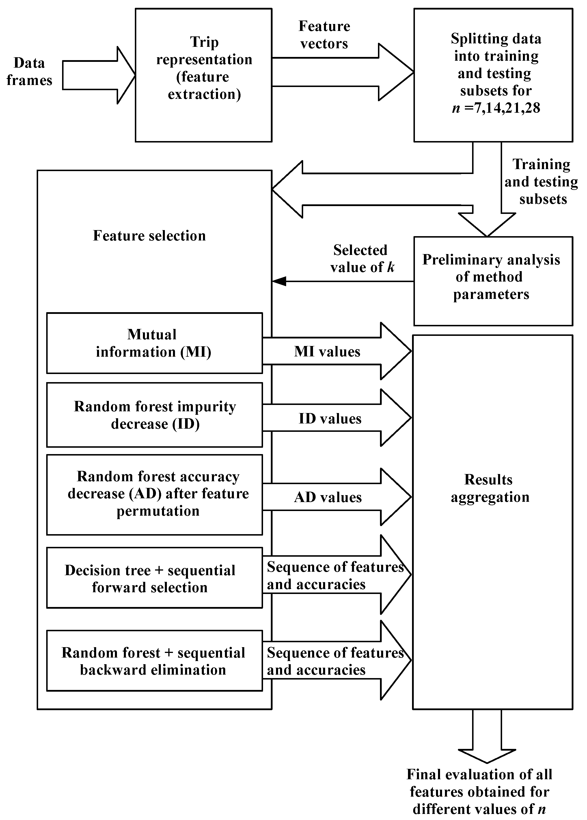Figure 2 shows a diagram presenting the whole process implemented to evaluate the impact of various factors on the changes of trip prices. The following subsections describe in detail the stages of that procedure and present the obtained results.

3.1. Trip Representation

The aim of the data set preparation stage, which was a highly time-consuming process, was to generate a set of feature vectors representing trips. The available raw data required a complex processing. The data originated from two tour operators identified as T1 and T2 in subsequent sections. Two types of trips, depending on the transport type, were taken into account, i.e., flight and own transport. Evaluation of features was performed independently for these two trip types. Due to huge amounts of available data, the first step was to sample a set of trips for future analysis. A few restrictions were imposed during the sampling process: no missing values were accepted, a trip was supposed to be offered at least 30 times and at least one price change should have been observed during the time the trip was offered. In this way, 51,419 (61% from T1) trips with flight transport and 34,839 (98% from T1) with their own transport were sampled.

Each trip was a source of a number of feature vectors. The available raw data enabled us to define a set of handcrafted features representing a trip at a given time. Such a representation vector of a trip in a given moment contained a set of constant parameters equal for all vectors generated on the basis of that trip and a set of varying parameters different for each vector originating from the given trip, depending on the day.

The constant parameters included accommodation and meal attributes, characteristics of local attractions, average weather parameters, season attributes indicating, for example, any holidays at the time of the trip, length of the trip, distance between the starting and destination locations and GDP per capita being a constant factor, because data were gathered during one year. Moreover, for trips with flight transport, several flight and airport attributes were incorporated.

Time-varying variables included trip price per person per day, macroeconomic indices, and current temperature, both in the starting and destination location. Moreover, a few additional features were extracted on the basis of raw data. It was delta denoting the number of days from the first day a trip was offered, changes denoting the number of times the trip’s price was already changed, days_till_departure denoting the number of days from the current day until the departure, and month denoting the current month.

For some of the time-varying parameters, seven new features were extracted to represent the rate of change of these variables. To do it, the best fit slope was calculated on the basis of k last values of the corresponding parameter. The new features representing the slope are called by adding a _serie suffix to the original name, e.g., barrel_price_serie was calculated on the basis of k last values of barrel_price. It was performed for $k=2,3,4,5,6,7$ to observe the influence of k on further results, which is shown further in Section 3.3.1.

To sum up, 56 features for trips with own transport and 60 for flight transport were extracted. The four flight attributes present only in the case of trips with flight transport were as follows: flight_type_name, airport_distance, destination_from_airport_passengers, and direct_flight.

The full list of features divided into groups is presented in Table 1.

Depending on the value of n and the values of k, training data sets of different sizes were created, as it is shown in Table 2. If, for example, a trip was offered from 1 April to 30 April, then at most 23 feature vectors for $n=7$ could be extracted on the basis of that trip, provided the trip was offered every day in April. Usually some gap days appeared during the lifetime of a trip. Therefore, the possible number of extracted vectors was usually lower. Table 2 presents numbers of feature vectors for $k=3$. For higher values of k, the sizes of data sets were lower, because higher values of k required longer sequences of days when a trip was offered continually, which was less likely.

The final stage of the preprocessing was transforming categorical features to numerical ones and normalizing all parameters.

Table 1. Feature set.

Features	Description
Constant parameters
length	Length of the trip in days
tour_distance	Distance between the starting and destination location
start_month, high_season, affected_by_holiday	Attributes of the season of the trip
hotel_chain, category, categorized, number_of_restaurants, child_attractiveness, hygiene, health_services, swimming_pool, golf_course, fitness	Hotel attributes
room_type, room_attractiveness, meal_code, persons_number, max_persons, room_kitchenette	Room attributes
heritage, historic, museum-gallery, attraction, UNESCO, protected_area, hiking, coastline, lake	Characteristics of local attractions
destination_to_departure_date_temp, destination_from_departure_date_temp, destination_to_avg_temp, destination_to_avg_rainfall, destination_to_avg_number_of_sunny_days, destination_to_avg_water_temp	Weather parameters describing the climate
destination_from_airport_passengers, airport_distance, flight_type_name, direct_flight	Flight and airport attributes, taken into account only for trips with flight transport
GDP per capita	GDP per capita in destination location, classified as a constant attribute, because data were originated from one year
Time varying parameters
personday_price	Trip price per person, per day
usd_avg	USD average exchange rate in zlotys
barrel_price	Oil price per barrel
Unemployment_Rate	Unemployment rate in destination location
Inflation_Rate	Inflation rate in destination location
Inflation_Rate_PL	Inflation rate in Poland, where the trips are offered
destination_to_current_temp	Temperature in the destination location
destination_from_current_temp	Temperature in the starting location
destination_to_current_temp_serie, destination_from_current_temp_serie, usd_avg_serie, barrel_price_serie, Inflation_Rate_serie, Inflation_Rate_PL_serie, Unemployment_Rate_serie	Parameters representing best fit slope for the selected time-varying parameters
delta	Number of days from the first day a trip was offered
changes	Number of times the trip’s price was already changed
month	Current month
days_till_departure	Number of days from the current day until the departure

Table 1. Feature set.

Features	Description
Constant parameters
length	Length of the trip in days
tour_distance	Distance between the starting and destination location
start_month, high_season, affected_by_holiday	Attributes of the season of the trip
hotel_chain, category, categorized, number_of_restaurants, child_attractiveness, hygiene, health_services, swimming_pool, golf_course, fitness	Hotel attributes
room_type, room_attractiveness, meal_code, persons_number, max_persons, room_kitchenette	Room attributes
heritage, historic, museum-gallery, attraction, UNESCO, protected_area, hiking, coastline, lake	Characteristics of local attractions
destination_to_departure_date_temp, destination_from_departure_date_temp, destination_to_avg_temp, destination_to_avg_rainfall, destination_to_avg_number_of_sunny_days, destination_to_avg_water_temp	Weather parameters describing the climate
destination_from_airport_passengers, airport_distance, flight_type_name, direct_flight	Flight and airport attributes, taken into account only for trips with flight transport
GDP per capita	GDP per capita in destination location, classified as a constant attribute, because data were originated from one year
Time varying parameters
personday_price	Trip price per person, per day
usd_avg	USD average exchange rate in zlotys
barrel_price	Oil price per barrel
Unemployment_Rate	Unemployment rate in destination location
Inflation_Rate	Inflation rate in destination location
Inflation_Rate_PL	Inflation rate in Poland, where the trips are offered
destination_to_current_temp	Temperature in the destination location
destination_from_current_temp	Temperature in the starting location
destination_to_current_temp_serie, destination_from_current_temp_serie, usd_avg_serie, barrel_price_serie, Inflation_Rate_serie, Inflation_Rate_PL_serie, Unemployment_Rate_serie	Parameters representing best fit slope for the selected time-varying parameters
delta	Number of days from the first day a trip was offered
changes	Number of times the trip’s price was already changed
month	Current month
days_till_departure	Number of days from the current day until the departure

Table 2. Sizes of data sets for various n and transport types, for $k=3$.

Touroperator	Transport	n = 7	n = 14	n = 21	n = 28	Features
T1	Own	1,758,117	1,683,516	1,547,542	1,406,752	56
	Flight	1,237,725	1,204,965	1,067,636	971,438	60
T2	Own	23,890	21,078	17,784	15,340	56
	Flight	621,135	545,807	514,031	417,984	60

Table 2. Sizes of data sets for various n and transport types, for $k=3$.

Touroperator	Transport	n = 7	n = 14	n = 21	n = 28	Features
T1	Own	1,758,117	1,683,516	1,547,542	1,406,752	56
	Flight	1,237,725	1,204,965	1,067,636	971,438	60
T2	Own	23,890	21,078	17,784	15,340	56
	Flight	621,135	545,807	514,031	417,984	60

3.2. Splitting Data into Training and Testing Subsets

The classification tasks defined, as it has been described, and constrained some requirements on the way of dividing data into training and testing subsets. Standard cross-validation was not appropriate in this case. The task corresponds to predicting price changes in future. To obtain unbiased error estimates, it was necessary to ensure that training samples referred to periods earlier than the testing ones. Therefore, several data splits have been applied and the results were averaged over these splits.

Table 3. Splitting data into training and testing subsets.

Split	Training Data	Test Data
		n = 7	n = 14	n = 21	n = 28
1	1 January–30 April	7 May–6 June	14 May–13 June	21 May–20 June	28 May–27 June
2	1 January–31 May	7 June–7 July	14 June–14 July	21 June–21 July	28 June–28 July
3	1 January–30 June	7 July–6 August	14 July–13 August	21 July–20 August	28 July–27 August
4	1 January–31 July	7 August–6 September	14 August–13 September	21 August–20 September	28 August–27 September
5	1 January–31 August	7 September–7 October	14 September–14 October	21 September–21 October	28 September–28 October
6	1 January–30 September	7 October–6 November	14 October–13 November	21 October–20 November	28 October–27 November

presents the time ranges covering successive splits of the data set into training and testing subsets.

3.3. Preliminary Analysis of Method Parameters

Before a thorough feature investigation, some preliminary analysis was performed in order to fix a value of series length k and to confirm that the selected classification methods were adequate for future analysis.

3.3.1. Series Length for Time Varying Features

The aim of this step was to evaluate the influence of parameter k on the quality of time-varying features, calculated as the best fit slopes on the basis of the last k values. Mutual information coefficient was chosen as a measure of usefulness of these features in the defined classification task. It measures the amount of information shared by the two variables together and is defined as follows [25]:

$$I(X;Y)=\sum _{x_i\in X}\sum _{y_i\in Y}P(x_i,y_i)log\frac{P(x_i,y_i)}{P\left(x_i\right)P\left(y_i\right)},$$

(1)

where $P(x_i,y_i)$ is the joint probability of $x_i$ and $y_i$. In this case, variables X and Y are the feature and the class.

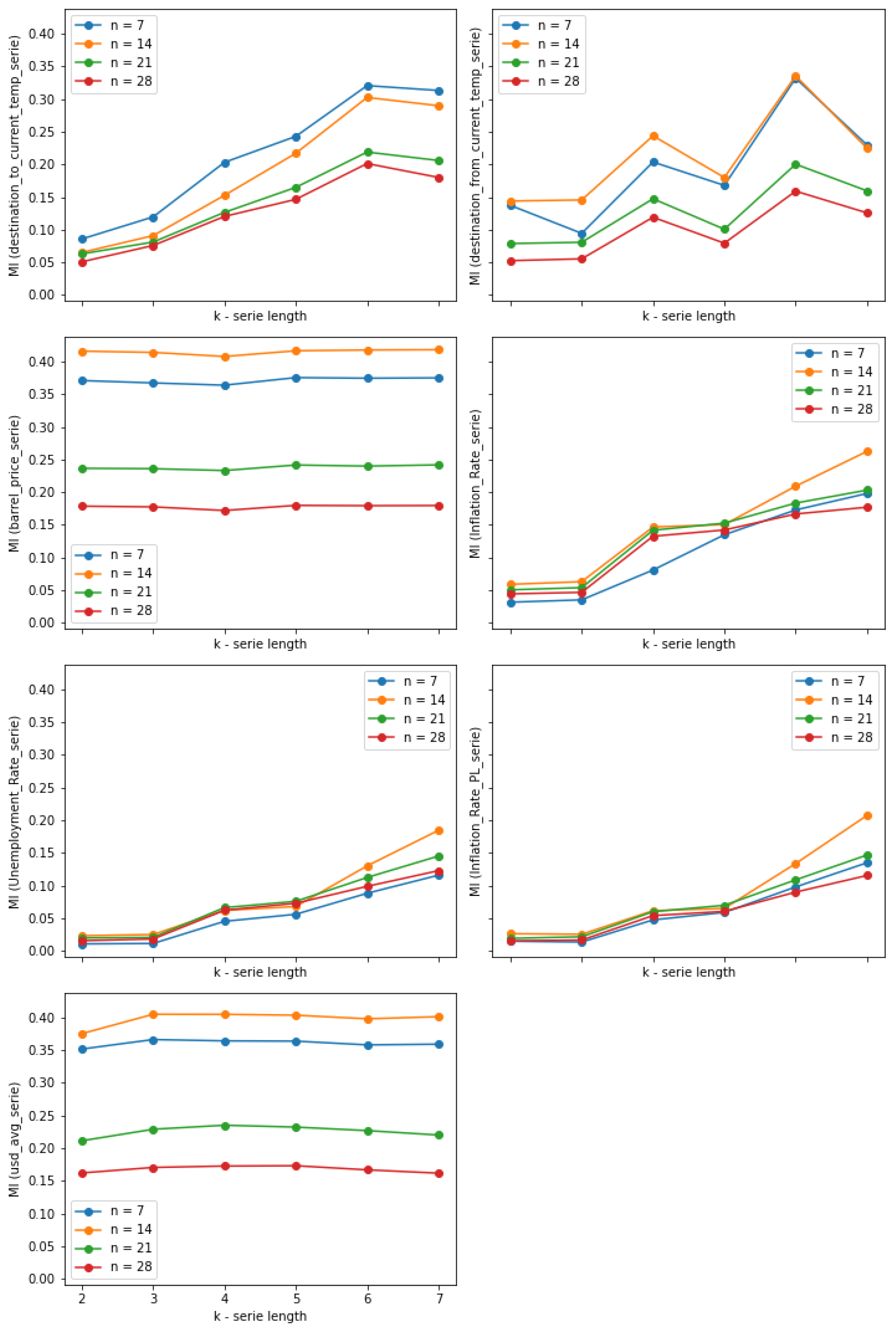
Figure 3 presents the values of the mutual coefficient for the seven features calculated on the basis of series of values depending on series length k. The dependency has been demonstrated for each value of n.

It can be observed that MI for barrel_price_serie and usd_avg_serie almost does not change for different values of k. For other features based on the series, higher values of k lead to higher MI, suggesting that longer series lead to better features in our classification problem. This regularity is less clear only for destination_from_current_temp_serie. However, it should be noted that the inflation and unemployment indices are updated no more than once a month. It means that the best fit slope calculated on the basis of values from the last several days is usually 0. The longer the series, the higher chance that any change in inflation or unemployment rate is observed. The low variance of these features based on the short series is the reason for lower MI. Another important observation is that usually lower values of n are associated with higher MI values, which means that the proposed features seem to be better predictors in the case of shorter forecast horizons.

3.3.2. Performance of Selected Classifiers

In the case of some feature selection methods, their effectiveness in the classification task is evaluated using a classifier. Before selecting features, the classifiers were trained on the basis of a full set of features in order to verify whether the classifiers chosen as evaluation models might achieve satisfying results. This step is necessary, because evaluating features on the basis of a weak classifier would not lead to finding good predictors.

A classifier chosen for this study was a random forest. According to the no free lunch theorem, no machine learning algorithm is universally better than any other [26]. The choice of method depends on the training goal, the type and amount of available training data. Random forests are known to achieve high accuracies in various application and they successfully cope with the large number of features of any types.

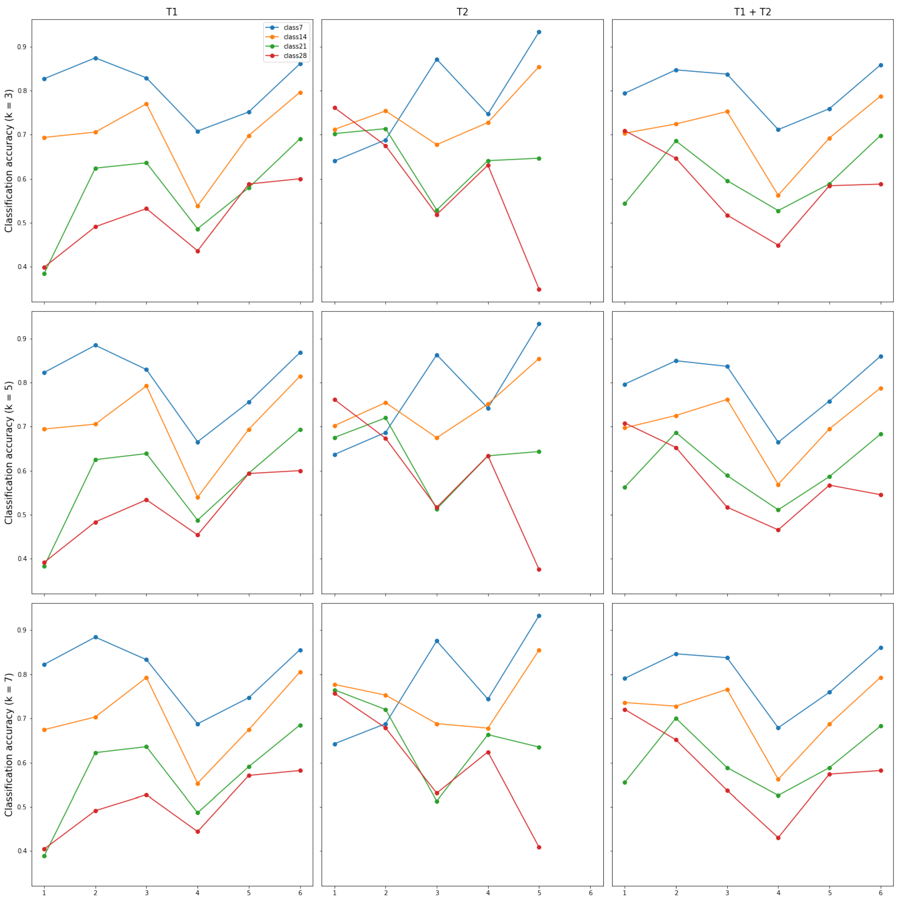
The numbers of samples in the splits were not equal, so any averages over splits were weighted averages. In each split, the training and test sets contained an equal number of samples per class. The training process was repeated six times for the splits defined in Table 3. Classification accuracies for each split, each data set and various series lengths are presented in Figure 4. The accuracies averaged over the splits and weighted by the number of feature vectors in the test sets, are shown in Figure 5. It has been performed for data from each tour operator separately and for the data set containing all vectors. More detailed results achieved for series length 3 are presented in

Table 4. Classification results for data from both tour operators and series length 3.

n	Metric	Down	No Change	Up	Avg
	Precision [%]	90.05	76.98	80.13	82.39
7	Recall [%]	74.14	87.24	80.15	80.51
	F1 score [%]	80.9	81.34	79.35	80.53
	Precision [%]	83.51	69.04	61.61	71.39
14	Recall [%]	70.97	66.07	68.72	68.59
	F1 score [%]	76.31	65.32	63.67	68.43
	Precision [%]	74.29	59.02	52.05	61.79
21	Recall [%]	59.47	51.17	63.89	58.18
	F1 score [%]	65.15	52.59	55.63	57.79
	Precision [%]	70.9	54.38	56.38	60.55
28	Recall [%]	56.74	59.16	58.52	58.14
	F1 score [%]	62.53	55.3	54.15	57.33

,

Table 5. Classification results [%] for data from tour operator T1 and series length 3.

n	Metric	Down	No Change	Up	Avg
	Precision [%]	89.05	82.03	78.67	83.25
7	Recall [%]	75.4	85.25	84.21	81.62
	F1 score [%]	81.19	83.07	80.6	81.62
	Precision [%]	77.66	81.67	60.05	73.13
14	Recall [%]	64.69	56.44	80.23	67.12
	F1 score [%]	69.45	63.12	66.8	66.46
	Precision [%]	63.64	57.71	48.03	56.46
21	Recall [%]	56.48	33.59	69.96	53.34
	F1 score [%]	57.76	40.22	55.31	51.1
	Precision [%]	52.78	49.56	53.74	52.03
28	Recall [%]	57.03	43.43	53.18	51.21
	F1 score [%]	53.87	44.83	50.96	49.89

and

Table 6. Classification results [%] for data from tour operator T2 and series length 3.

n	Metric	Down	No Change	Up	Avg
	Precision [%]	99.6	55.27	98.55	84.47
7	Recall [%]	64.35	99.14	49.78	71.09
	F1 score [%]	77.01	70.4	62.05	69.82
	Precision [%]	95.59	56.88	87.85	80.11
14	Recall [%]	84.76	93.49	38.36	72.2
	F1 score [%]	89.64	70.32	50.73	70.23
	Precision [%]	93.97	53.92	69.59	72.49
21	Recall [%]	69.92	84.87	46.12	66.97
	F1 score [%]	79.66	65.03	53.89	66.19
	Precision [%]	92.68	64.53	61.95	73.05
28	Recall [%]	64.32	76.27	63.35	67.98
	F1 score [%]	75.08	68.96	58.22	67.42

, where the values of metrics such as precision, recall and F1-score, calculated separately for each class and averaged over classes, are presented.

The presented results demonstrated that the smaller n, the higher classification accuracy, which can be observed especially for data from tour operator T1 and for the combined set of feature vectors. It is not equally clear for tour operator T2, but it should be noted that the number of data from T2 is lower than from T1. It can be also said that some splits, i.e., split 4 and 5, show much lower accuracies. In the case of data from tour operator T2, there were very little samples for split 5 and $n=28$, which resulted in low accuracy, and can be observed in Figure 4; for split 6, there were not enough data samples from T2 to train the models at all. The highest scores obtained for $n=7$ exceed 80% for each metric. The lowest results obtained for $n=28$ are slightly below 60%, which is still much higher than a random guess in the case of three classes. Such results demonstrate that the classifiers might be chosen as evaluation models during the feature selection process.

The other important observation is that there are no significant differences between the results for different series lengths k, even if some relation between k and mutual information was discovered for inflation and unemployment rates, as it was shown in Section 3.3.1. This observation led us to choose $k=3$ for further experiments on feature selection. Lower value of k let us to achieve larger data sets, as it has already been mentioned.

3.4. Feature Selection

Feature selection is the process of reducing the size of the set containing all original attributes describing the data. The dimensionality reduction achieved in this way not only reduces the computational and space complexity, but may also influence the accuracy of the trained model, which may have better generalization ability. Feature selection methods fall into one of the following categories:

• Filter methods apply an evaluation function measuring the dependence between a given feature and a target value. Example criteria used as the evaluation function are Pearson coefficient, Spearman coefficient, mutual information. The advantage of filter methods is their low computational cost, but the drawback is the fact that they treat the predictors independently, neglecting potential correlations between them. A feature that is useless alone may be significant in combination with other features [27].
• Wrapper methods apply a trained model to evaluate the effectiveness of a selected feature subset. Depending on a given task, the model may be either a classifier or a regression model. These methods require choosing a feature space search strategy, leading to an iterative process. In each iteration, a new subset of features is generated, a model is trained and the subset is evaluated according to the model’s performance. Searching the whole space of feature subsets is infeasible; therefore, some heuristics are applied. One of the most popular ones are sequential methods, where in each iteration, features are either added to or removed from the current subset. The computational cost of wrapper methods is high, due to the need of training a model whenever a new subset of features has to be evaluated. To reduce the computational complexity, the recursive feature elimination proposed in [28] may be applied. This algorithm reduces the necessary number of repetitions of the model training procedure. In each stage, after creating a model, features are ranked and the least important predictor is eliminated. Then, the model is rebuilt on the basis of the reduced set of features.
• Embedded methods are feature selection algorithms constituting integral parts of the model training procedures. These are, for example, decision trees, where at each step of the decision tree construction, a feature is selected on the basis of a criterion, e.g., Gini index; or LASSO, which is able to find a linear regression model reducing the coefficients of some parameters to zero.

One might say that deep learning models applied nowadays do not require any feature selection procedure before training the model. However, even in this case it is a good idea to remove irrelevant features before training the model to reduce space and time complexity. Moreover, neural networks are blackbox models, which do not enable one to interpret the meaning of particular inputs. There are applications where some interpretation of the obtained knowledge representation is valuable or even required. Finally, knowledge about irrelevant parameters might prevent one from collecting unnecessary data in future, which might result not only in reducing the required space but also costs the data collection process.

During the performed experiments, the following feature selection methods have been implemented:

1.

Filter method with mutual information criterion to evaluate the dependence between a feature’s values and classes;

2.

Embedded method with a random forest enabling to assign weights to the features on the basis of a mean decrease in impurity;

3.

Random forest letting one assign weights to the features on the basis of a decrease in the forest’s accuracy after a random permutation of a feature’s value;

4.

Wrapper method with sequential forward selection as a search strategy and a decision tree as a classification model;

5.

Wrapper method with recursive feature elimination as a search strategy and a random forest as a classification model.

Is is worth mentioning that all implemented methods are supervised methods, i.e., class labels are taken into account in the process of feature selection, either by calculating some correlation between features and classes or by applying a classification model to inspect the power of features in the given classification task. In general, feature selection might also be implemented in an unsupervised manner, but this type of selection is designed for clustering problems, which is not in this case [25].

In the case of embedded methods, decision trees or random forests, which are ensembles of decision trees, were selected [29]. These ensembles are sets of decision trees, that differ thanks to applying two types of randomness. The first one is bagging, which means that the training set for each tree is drawn, with replacement, from the original data. The second is the random selection of features at each node to define the splitting rule. Random forests are known to achieve a low generalization error, especially in classification tasks. In the case of sequential forward selection, we chose the decision tree instead of the random forest to reduce the time-complexity of this procedure.

3.5. Results’ Aggregation

Although the aim of all methods mentioned above was the same, the obtained results might vary more or less. Therefore, it was necessary to propose an algorithm able to summarize the results generated by the five methods and present a final feature ranking. In the case of the first three feature selection methods, the features are assigned values, which may be treated as weights, i.e., higher mutual information or impurity reduction mean better discriminative power of a given feature. These values have been normalized to a range of $[0,1]$. In the case of sequential methods, no weights have been extracted, but the wrapper approach lets us select a subset of features that enables for creating a prediction model demonstrating satisfying accuracy. We assign 1 to the features selected by a sequential method and 0 to all the others. 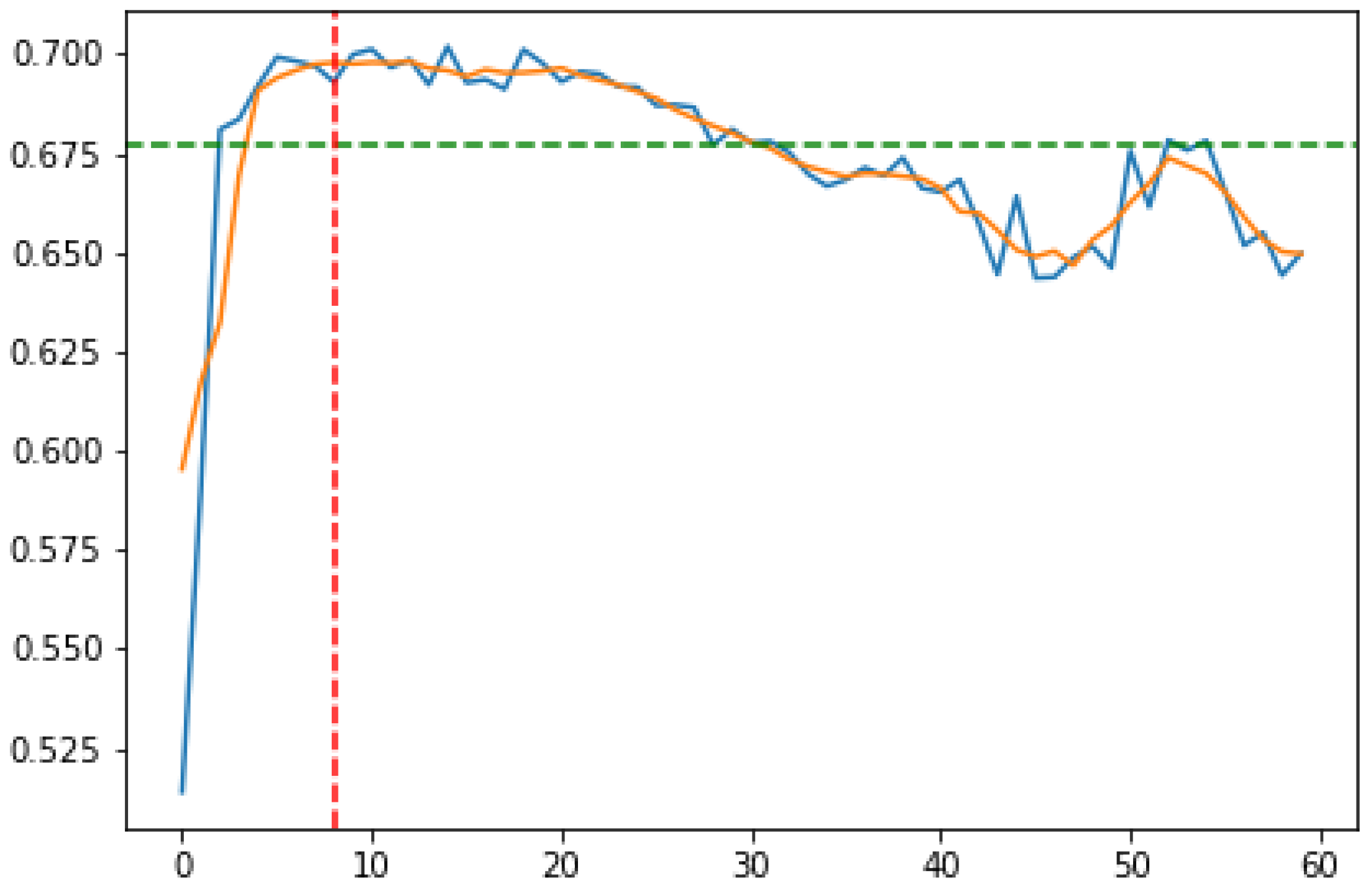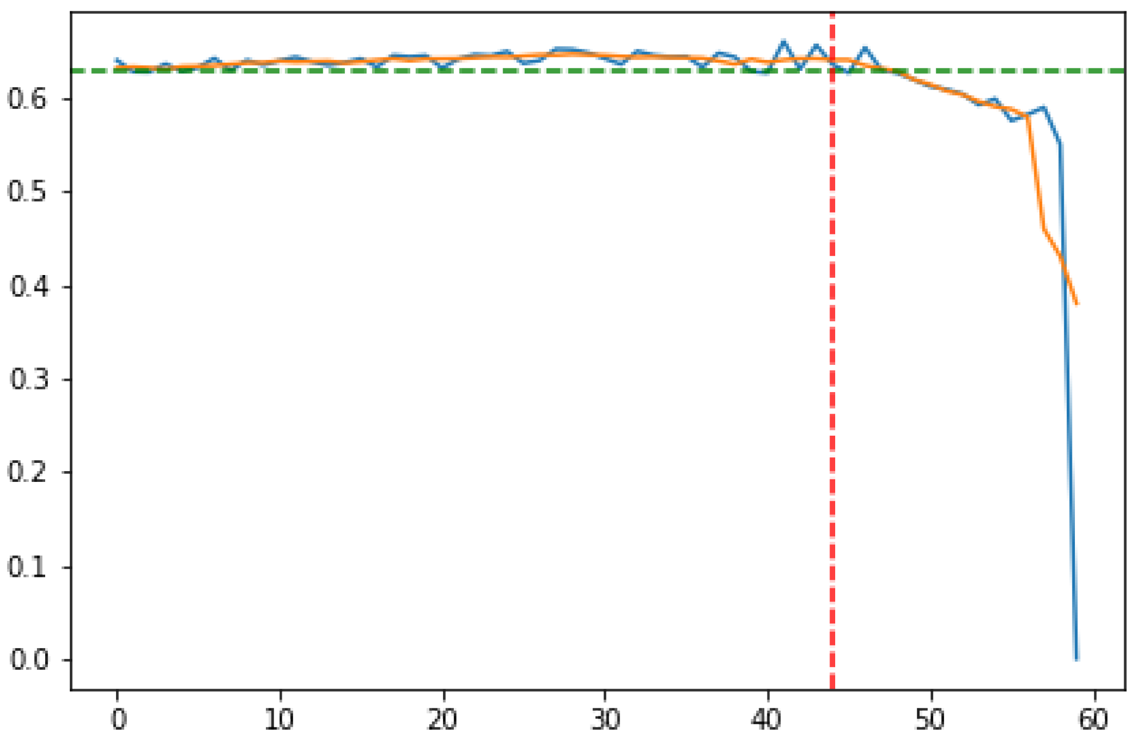Figure 6 and Figure 7 present the way an optimal subset of features is selected during the sequential procedure. The graphs are generated for an example subset of flight trips data. The proposed method is as follows:

1.

For each iteration of the sequential feature selection, the algorithm estimates the accuracy of the wrapper model on the basis of a separate test set (blue lines on Figure 6 and Figure 7).

2.

Smooth the series obtained in the previous step using the moving average of width 5 (orange lines).

3.

In the case of the sequential forward selection (Figure 6), identify the initial segment of the series, where the accuracy increases by at least 1 pp in each subsequent iteration. In the case of the sequential backward selection (Figure 7), identify the ending fragment of the series, where the accuracy decreases by at least 1 pp in each iteration.

4.

Omit the fragment of the series identified in the previous step and calculate the average value on the basis of the remaining part. These values are marked with green dashed lines on Figure 6 and Figure 7.

5.

In the case of sequential forward selection (Figure 6), find the fifth feature, which makes the accuracy exceed the average value determined in the previous step. In the case of the sequential backward selection (Figure 7), find the feature, after removing which five more can be removed without dropping the accuracy below the average value determined in the previous step. The feature (iteration) identified in this way is marked with red dashed lines.

6.

In the case of sequential forward selection, select the features from the first to the one identified in the previous step. In the case of the sequential backward selection, select the features starting from the one identified in the previous step to the last one.

As it has been mentioned in Section 3.4, five feature selection methods have been applied in order to evaluate the features. In the results, each method assigned a weight value $Wi$ to every predictor, indicating its ability to predict whether the trip price would go up, down or remain unchanged. The weights are:

• $W1$—weight assigned according to mutual information value;
• $W2$—weight assigned on the basis of a mean decrease in the impurity of a random forest;
• $W3$—weight assigned according to the decrease in a random forest’s accuracy after feature values permutation;
• $W4$—weight assigned on the basis of the results of the sequential forward selection method;
• $W5$—weight assigned on the basis of the results of the sequential backward elimination method.

Weight $W1$ was calculated only once for the whole set of data. The other four weights required model training and testing to evaluate accuracy. In these cases, the evaluation was performed for all five splits and the resulting weight values were averaged over the splits. Split 6 was omitted, because there were not enough data samples from T2 in the corresponding subset.

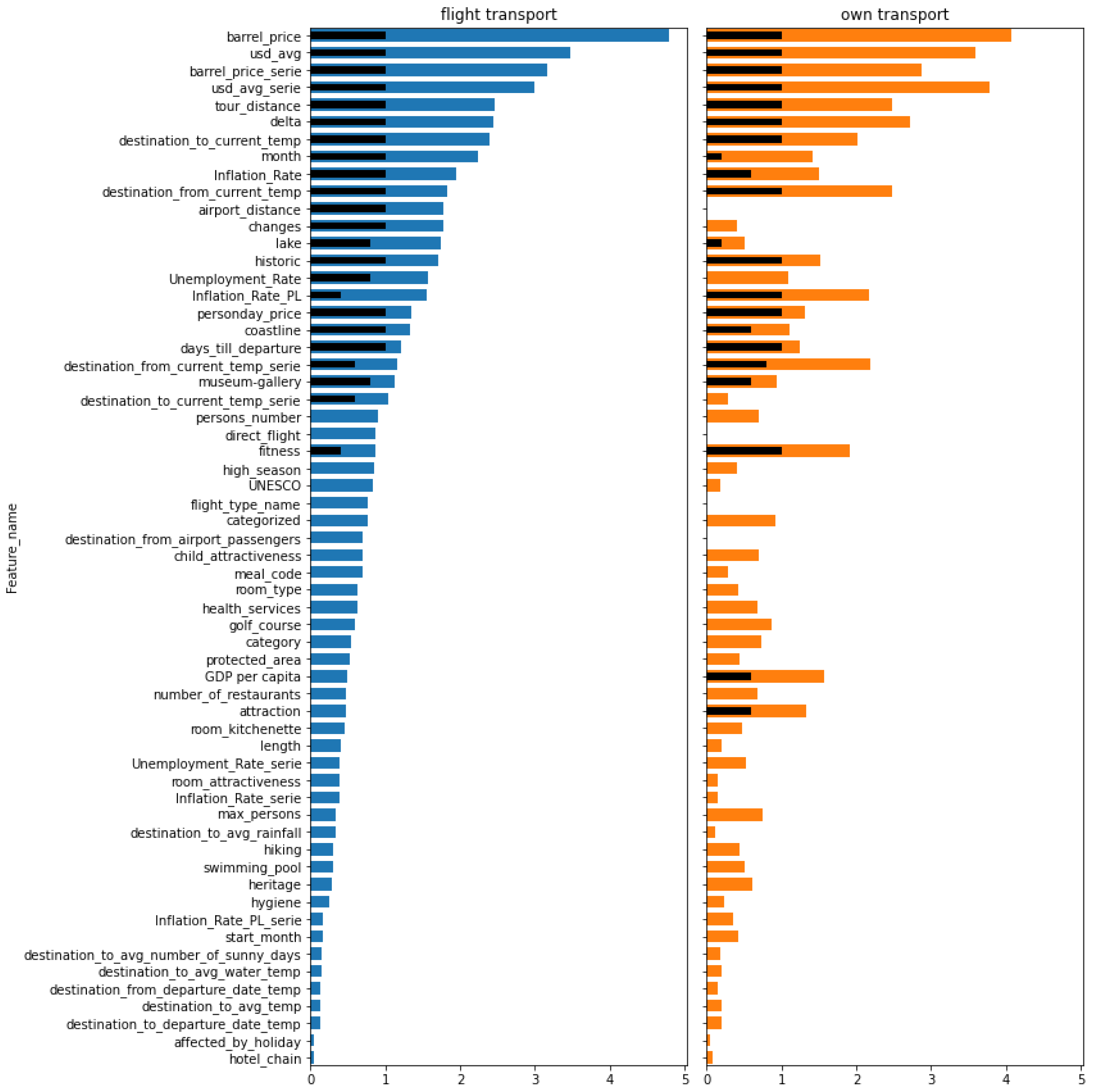
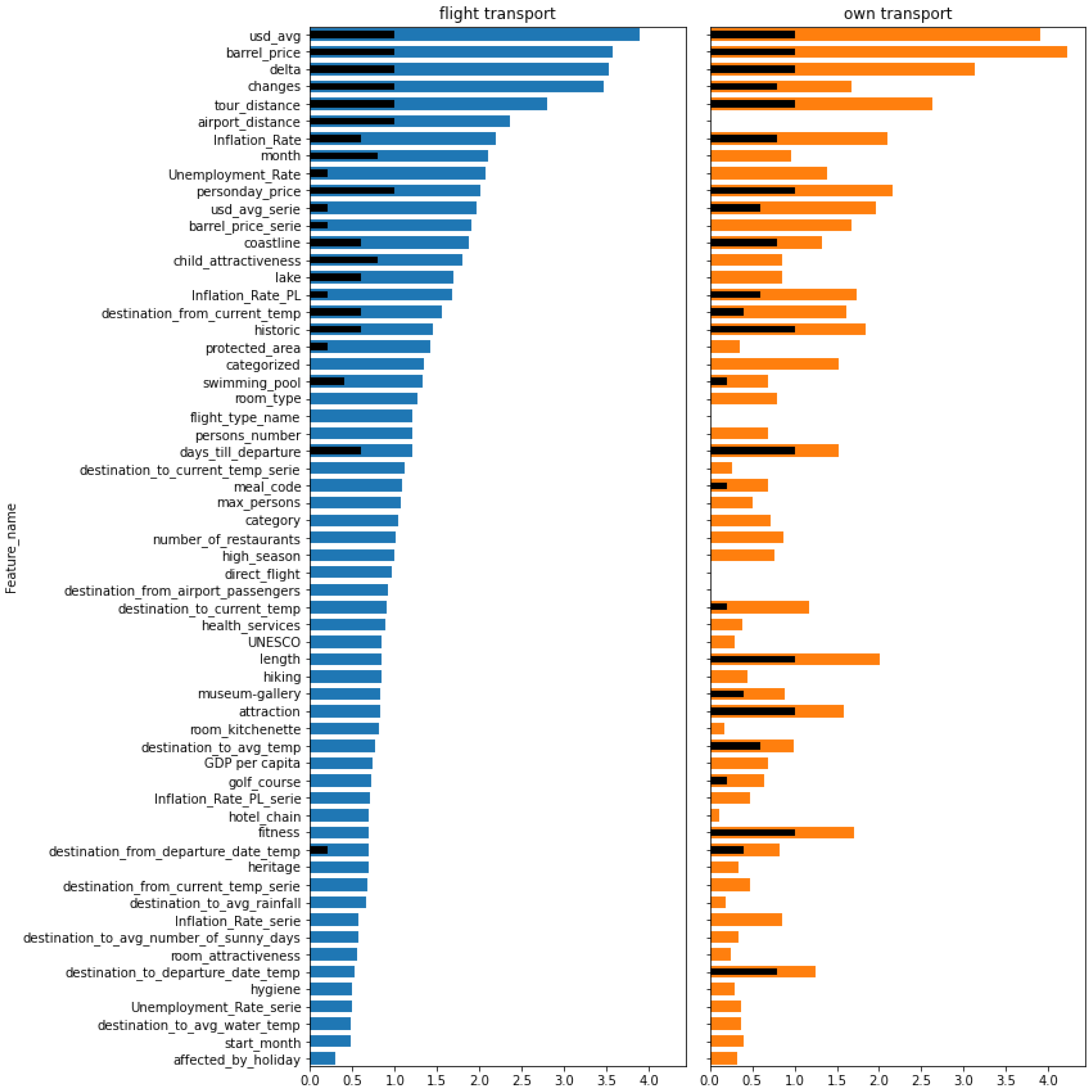
To obtain the final evaluation, the sum of the weights was taken into account.

Table A1. Features’ weights assigned for four classification problems and two types of transport.

Feature	Transport Type: Flight				Transport Type: Own
	n = 7	n = 14	n = 21	n = 28	n = 7	n = 14	n = 21	n = 28
direct_flight	0.87	0.72	0.9	0.96	-	-	-	-
room_type	0.63	0.32	1.0	1.27	0.42	0.39	0.73	0.79
meal_code	0.69	0.24	0.65	1.08	0.28	0.3	0.43	0.69
persons_number	0.9	0.77	0.9	1.21	0.7	0.67	1.04	0.69
max_persons	0.33	0.47	0.79	1.07	0.75	0.55	0.86	0.51
length	0.4	0.24	0.56	0.84	0.2	0.58	1.75	2.01
flight_type_name	0.77	0.73	0.75	1.21	-	-	-	-
personday_price	1.34	1.3	1.75	2.01	1.31	1.55	2.12	2.16
room_attractiveness	0.39	0.18	0.56	0.56	0.14	0.18	0.22	0.25
airport_distance	1.77	1.75	2.1	2.36	-	-	-	-
destination_from_airport_passengers	0.69	0.38	0.82	0.91	-	-	-	-
high_season	0.85	0.53	0.8	0.99	0.4	0.78	0.91	0.76
destination_to_current_temp	2.39	2.13	1.43	0.9	2.02	1.14	1.36	1.17
destination_to_departure_date_temp	0.12	0.15	0.34	0.52	0.19	0.69	1.03	1.24
destination_from_current_temp	1.82	2.24	2.38	1.56	2.48	3.17	2.36	1.62
destination_from_departure_date_temp	0.13	0.17	0.53	0.69	0.15	0.24	0.77	0.82
destination_to_avg_temp	0.13	0.17	0.36	0.76	0.2	0.7	0.96	0.99
destination_to_avg_rainfall	0.33	0.32	0.47	0.66	0.11	0.14	0.15	0.19
destination_to_avg_number_of_sunny_days	0.15	0.15	0.6	0.56	0.17	0.22	0.29	0.34
destination_to_avg_water_temp	0.14	0.18	0.35	0.48	0.2	0.28	0.33	0.37
days_till_departure	1.2	0.87	1.51	1.21	1.24	1.14	1.51	1.53
affected_by_holiday	0.04	0.08	0.37	0.3	0.05	0.09	0.08	0.32
tour_distance	2.46	2.41	2.88	2.79	2.49	2.52	2.65	2.63
usd_avg	3.48	4.08	3.64	3.89	3.6	3.36	3.24	3.9
barrel_price	4.79	4.6	4.13	3.57	4.08	4.24	4.19	4.23
GDP per capita	0.49	0.26	0.99	0.74	1.57	0.58	0.66	0.69
destination_to_current_temp_serie	1.04	0.35	0.76	1.11	0.28	0.23	0.45	0.26
destination_from_current_temp_serie	1.16	0.58	0.53	0.67	2.18	0.82	0.92	0.48
usd_avg_serie	2.99	1.99	2.33	1.96	3.79	2.64	2.6	1.96
barrel_price_serie	3.16	2.4	2.75	1.91	2.88	2.2	2.33	1.68
Inflation_Rate_serie	0.38	0.43	0.57	0.57	0.15	0.43	0.4	0.85
Unemployment_Rate_serie	0.39	0.4	0.52	0.49	0.52	0.36	0.13	0.37
Inflation_Rate_PL_serie	0.16	0.24	0.48	0.7	0.35	0.47	0.2	0.47
delta	2.44	2.45	3.11	3.53	2.72	2.53	3.21	3.13
hotel_chain	0.04	0.28	0.36	0.7	0.07	0.49	0.86	0.12
category	0.54	0.48	0.79	1.04	0.73	0.33	0.67	0.72
categorized	0.76	0.4	1.05	1.35	0.92	0.69	0.66	1.53
room_kitchenette	0.46	0.11	0.41	0.82	0.48	0.33	0.11	0.18
number_of_restaurants	0.48	0.37	0.87	1.01	0.68	0.65	0.61	0.87
child_attractiveness	0.69	0.46	1.18	1.8	0.69	0.47	0.78	0.85
hygiene	0.24	0.28	0.36	0.5	0.24	0.3	0.05	0.3
health_services	0.62	0.41	0.46	0.88	0.67	1.07	0.75	0.38
swimming_pool	0.31	0.86	1.09	1.33	0.5	0.92	0.63	0.68
golf_course	0.59	0.18	0.55	0.73	0.87	0.5	0.37	0.64
fitness	0.87	1.06	0.9	0.69	1.91	1.59	1.67	1.7
heritage	0.28	0.41	0.53	0.69	0.61	0.45	0.49	0.34
historic	1.71	0.87	1.51	1.45	1.52	1.58	1.57	1.85
museum-gallery	1.13	0.29	1.26	0.83	0.93	1.34	0.62	0.88
attraction	0.47	0.46	0.7	0.82	1.33	1.2	1.77	1.59
UNESCO	0.84	0.4	0.49	0.85	0.18	0.22	0.24	0.29
protected_area	0.52	0.44	0.63	1.42	0.43	0.25	0.32	0.35
hiking	0.31	0.47	0.64	0.84	0.44	0.68	1.39	0.45
coastline	1.32	1.25	1.52	1.88	1.1	0.54	1.05	1.32
lake	1.73	0.88	1.07	1.7	0.5	0.5	0.61	0.86
Inflation_Rate	1.95	1.65	2.05	2.19	1.5	2.27	2.51	2.1
Unemployment_Rate	1.57	0.65	1.83	2.06	1.09	0.75	1.41	1.38
Inflation_Rate_PL	1.55	1.12	2.64	1.67	2.17	1.92	2.29	1.74
changes	1.77	2.0	2.51	3.46	0.41	0.95	1.49	1.67
month	2.23	1.73	2.63	2.11	1.42	0.69	1.08	0.96
start_month	0.16	0.16	0.32	0.48	0.42	0.26	0.33	0.4

presents the summary values for each feature obtained for each value of n and for both sets of data, i.e., those with flight and their own transport type. The summary results have been also presented in Figure 8, Figure 9, Figure 10 and Figure 11 for $n=7,14,21,28$, respectively. Features on these bar plots are sorted according to the results obtained for trips with flight transport. Due to large amounts of results, the detailed values obtained by applying individual methods are presented only for top 10 features identified for each value of n both for the flight (

Table A2. Results obtained for top 10 features identified in each classification problem for trips with flight transport.

n	Feature	W1	W2	W3	W4	W5	∑
	barrel_price	1.0	1.0	0.99	1.0	0.8	4.79
	usd_avg	0.99	0.7	0.59	1.0	0.2	3.48
	barrel_price_serie	0.93	0.49	0.14	1.0	0.6	3.16
	usd_avg_serie	0.92	0.4	0.27	1.0	0.4	2.99
7	tour_distance	0.15	0.23	0.08	1.0	1.0	2.46
	delta	0.56	0.7	0.18	1.0	0.0	2.44
	destination_to_current_temp	0.34	0.57	0.28	1.0	0.2	2.39
	month	0.38	0.38	0.28	1.0	0.2	2.23
	Inflation_Rate	0.46	0.22	0.07	1.0	0.2	1.95
	destination_from_current_temp	0.3	0.4	0.13	1.0	0.0	1.82
	barrel_price	1.0	1.0	0.8	1.0	0.8	4.6
	usd_avg	1.0	0.76	0.72	1.0	0.6	4.08
	delta	0.61	0.57	0.27	1.0	0.0	2.45
	tour_distance	0.13	0.19	0.08	1.0	1.0	2.41
14	barrel_price_serie	0.91	0.31	0.18	0.8	0.2	2.4
	destination_from_current_temp	0.37	0.5	0.17	1.0	0.2	2.24
	destination_to_current_temp	0.34	0.44	0.16	0.8	0.4	2.13
	changes	0.32	0.47	0.21	1.0	0.0	2.0
	usd_avg_serie	0.92	0.34	0.14	0.6	0.0	1.99
	airport_distance	0.11	0.15	0.09	1.0	0.4	1.75
	barrel_price	1.0	1.0	0.73	1.0	0.4	4.13
	usd_avg	0.98	0.65	0.41	1.0	0.6	3.64
	delta	0.75	0.77	0.38	1.0	0.2	3.11
	tour_distance	0.44	0.39	0.26	1.0	0.8	2.88
21	barrel_price_serie	0.98	0.39	0.17	0.6	0.6	2.75
	Inflation_Rate_PL	0.54	0.45	0.26	0.8	0.6	2.64
	month	0.54	0.41	0.28	1.0	0.4	2.63
	changes	0.43	0.62	0.46	1.0	0.0	2.51
	destination_from_current_temp	0.44	0.68	0.27	1.0	0.0	2.38
	usd_avg_serie	0.84	0.38	0.31	0.6	0.2	2.33
	usd_avg	0.95	0.71	0.63	1.0	0.6	3.89
	barrel_price	0.96	0.82	0.79	1.0	0.0	3.57
	delta	0.8	0.72	0.61	1.0	0.4	3.53
	changes	0.47	0.95	0.65	1.0	0.4	3.46
28	tour_distance	0.53	0.57	0.29	1.0	0.4	2.79
	airport_distance	0.43	0.44	0.3	1.0	0.2	2.36
	Inflation_Rate	0.8	0.35	0.25	0.6	0.2	2.19
	month	0.5	0.53	0.28	0.8	0.0	2.11
	Unemployment_Rate	1.0	0.25	0.22	0.2	0.4	2.06
	personday_price	0.19	0.4	0.43	1.0	0.0	2.01

) and their own transport (

Table A3. Results obtained for top 10 features identified in each classification problem for trips with own transport.

n	Feature	W1	W2	W3	W4	W5	∑
	barrel_price	1.0	1.0	0.68	1.0	0.4	4.08
	usd_avg_serie	0.91	0.74	0.53	1.0	0.6	3.79
	usd_avg	0.99	0.8	0.61	1.0	0.2	3.6
	barrel_price_serie	0.92	0.62	0.13	1.0	0.2	2.88
7	delta	0.41	0.68	0.23	1.0	0.4	2.72
	tour_distance	0.1	0.29	0.1	1.0	1.0	2.49
	destination_from_current_temp	0.4	0.63	0.24	1.0	0.2	2.48
	destination_from_current_temp_serie	0.28	0.47	0.23	0.8	0.4	2.18
	Inflation_Rate_PL	0.33	0.48	0.16	1.0	0.2	2.17
	destination_to_current_temp	0.15	0.44	0.43	1.0	0.0	2.02
	barrel_price	1.0	1.0	0.44	1.0	0.8	4.24
	usd_avg	0.98	0.75	0.62	1.0	0.0	3.36
	destination_from_current_temp	0.46	0.78	0.92	1.0	0.0	3.17
	usd_avg_serie	0.88	0.48	0.28	0.8	0.2	2.64
14	delta	0.45	0.68	0.21	1.0	0.2	2.53
	tour_distance	0.15	0.28	0.09	1.0	1.0	2.52
	Inflation_Rate	0.5	0.19	0.18	0.6	0.8	2.27
	barrel_price_serie	0.92	0.35	0.13	0.6	0.2	2.2
	Inflation_Rate_PL	0.32	0.32	0.28	0.6	0.4	1.92
	fitness	0.06	0.17	0.16	0.6	0.6	1.59
	barrel_price	1.0	0.99	1.0	1.0	0.2	4.19
	usd_avg	0.95	0.58	0.52	1.0	0.2	3.24
	delta	0.59	0.83	0.39	1.0	0.4	3.21
	tour_distance	0.28	0.48	0.09	1.0	0.8	2.65
21	usd_avg_serie	0.81	0.47	0.13	1.0	0.2	2.6
	Inflation_Rate	0.88	0.29	0.14	1.0	0.2	2.51
	destination_from_current_temp	0.49	0.51	0.16	1.0	0.2	2.36
	barrel_price_serie	0.96	0.49	0.07	0.6	0.2	2.33
	Inflation_Rate_PL	0.53	0.5	0.26	0.8	0.2	2.29
	personday_price	0.13	0.77	0.23	1.0	0.0	2.12
	barrel_price	1.0	1.0	0.83	1.0	0.4	4.23
	usd_avg	0.96	0.85	0.89	1.0	0.2	3.9
	delta	0.61	0.71	0.41	1.0	0.4	3.13
	tour_distance	0.3	0.4	0.12	1.0	0.8	2.63
28	personday_price	0.13	0.75	0.27	1.0	0.0	2.16
	Inflation_Rate	0.86	0.26	0.18	0.8	0.0	2.1
	length	0.07	0.49	0.25	1.0	0.2	2.01
	usd_avg_serie	0.85	0.33	0.18	0.6	0.0	1.96
	historic	0.26	0.28	0.11	1.0	0.2	1.85
	Inflation_Rate_PL	0.53	0.25	0.17	0.6	0.2	1.74

) transport type.

3.6. Discussion

First of all, it should be mentioned that the two types of features, i.e., time-varying and constant ones, play different roles in solving the stated classification problem. Time-varying parameters are obviously those that may have an impact on the price changes. Constant parameters, on the other hand, may cluster data into various groups, where the prices follow different rules. In our experiments, we analyzed all of them together, as most of the applied methods are tree-based methods, where the feature space is sequentially partitioned on the basis of selected features. In that way, data from various space regions may traverse various decision paths on the basis of all available parameters. Another possible approach could be applying a clustering algorithm only on the basis of constant attributes and then train a separate classifier for each cluster on the basis of time-varying features.

Feature rankings obtained for the different values of n do not vary much. The current price per oil barrel (barrel_price) and USD average exchange rate (usd_avg) are at the top in each case of n, both for the flight and own transport type. An interesting observation is made for features representing the rate of changes of the above two parameters, i.e., barrel_price_serie and usd_avg_serie. They are also significant predictors, as they usually appear in the top 10 subsets, but it can be observed that the lower n, the higher the position of these two features. It means they are better in shorter time predictions. Another essential predictor is delta, representing the number of days a trip is already offered. In each case, it takes places from three to five, no matter the transport type and the value of n. Among features that are not time-varying, the tour_distance is the most significant, no matter the transport type. Weather features did not turn out to be important. They usually fall at the end of the ranking list. The only exceptions are current temperatures in the destination and the starting location (destination_to_current_temp and destination_from_current_temp) in the case of flight trips for $n=7$. This means that changes of weather are not essential for more predictions in the longer horizon. Comparisons between trips with flight and own transport indicate strong similarities. The same parameters are on the top of the ranking lists. There are several features that are often higher in the case of their own transport. These are fitness, attraction, and Inflation_rate_PL. On the other hand, month and changes appear to be better predictors in the case of flight transport. Apart from the fitness, which has already been mentioned, other hotel attributes do not demonstrate a high significance in solving the classification task.

It is also interesting to analyze the results of the sequential backward elimination, which is one of the wrapper methods that lets us find a subset optimal from the point of view of the accuracy of the applied model. The weights assigned to the features using this algorithm have been demonstrated using black bars in Figure 8, Figure 9, Figure 10 and Figure 11. To indicate an optimal m-element subset of features, it is important to make sure that the set of the top m predictors presented on the obtained ranking list contain a complete subset of features identified by the sequential method. There might be a feature, which has the discriminative power in combination with others, but individually it does not appear to be significant. Such a feature would not achieve high results using the methods that treat features independently, but it would using the method that takes into account feature correlations, e.g., sequential backward elimination. It can be observed that in the case of our data, the subsets selected by sequential backward elimination and on the basis of all methods together usually overlap to a great extent, especially for lower values of n. For larger n, this correlation is lower. For $n=28$, there are several features achieving low results with the sequential method, but are quite high in total. In the case of flight transport, these parameters in are: Unemployment_rate, usd_avg_serie, barrel_price_serie, Inflation_rate_PL, protected_area and catgorized. In the case of own transport these are: Unemployment_rate, month, barrel_price_serie, categorized and, destination_to_current_temp.

It should be noted that the two tour operators, which were the source of data sets, offered selected types of trips; therefore, any conclusions that are drawn from the presented analysis might refer to those trip types. However, a similar methodology might be applied for another data set.

4. Model of the Price Change Process

As it is known from the previous sections, a trip is a basic data unit, and the price is its attribute that can change over time. The rest of the trip attributes are created based on factors that hypothetically affect the price, which can be constant or changing over time, within a single trip lifetime.

The first step of modeling business processes is the ability to define the sequence of distinguishable events. The event has a specified beginning and an end, and after its completion, another event can be performed according to a workflow defined a priori or ad hoc. Events can be performed sequentially or in parallel, and can also describe a single action (e.g., click “send”) as well as some task to be performed (e.g., send a package to a customer). Hence, in order to model processes, it is necessary to change the attributes over a time, which causes the workflow to shift from one state to another.

The solution described in this section is to model the price change process using process mining techniques [4]. The price is expressed by two factors of the trip: baseprice and personday_price. From both of these factors, it is possible to calculate whether the price has increased or decreased. The increase and decrease in the price—not the value of the price difference—are recorded as events. The personday_price was selected for further research as, according to experts from the tourism industry, it is more reliable. Both prices change proportionally and can therefore be used interchangeably.

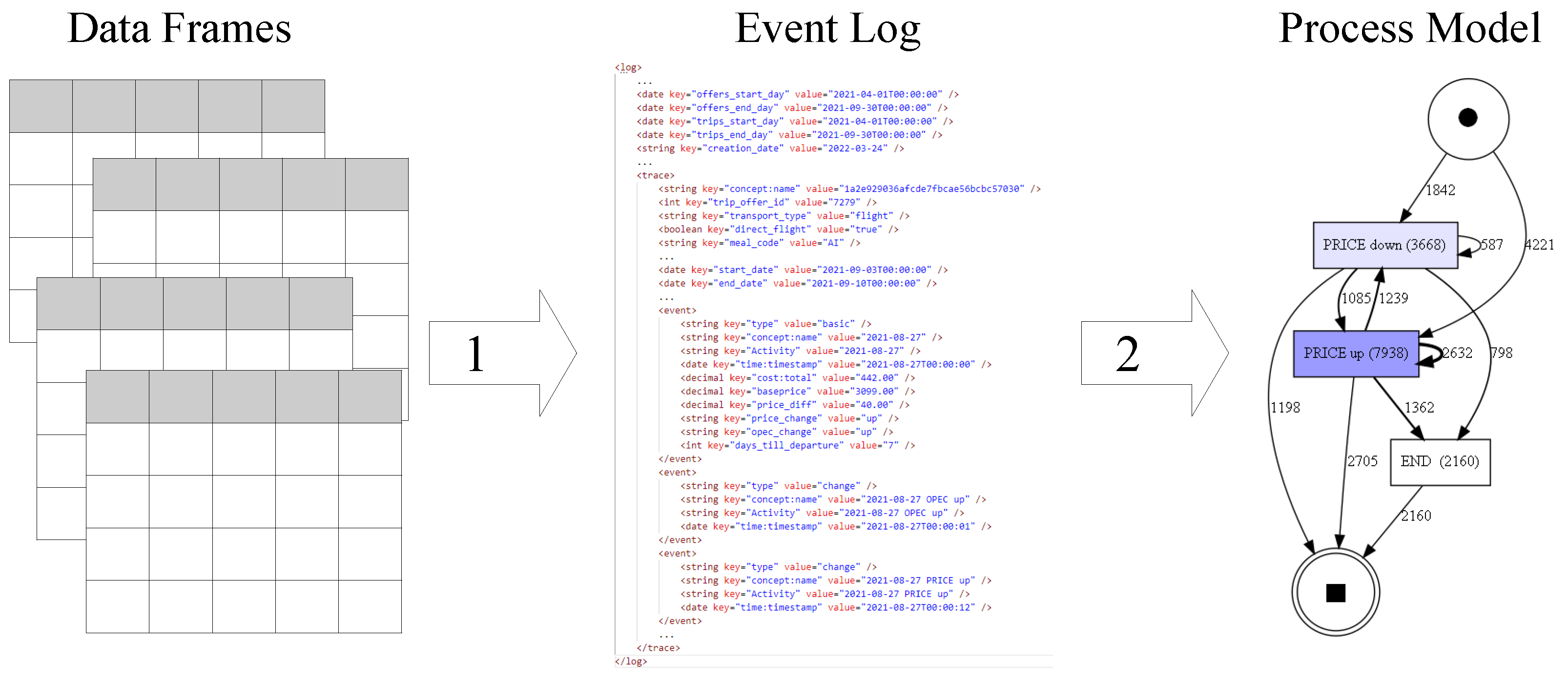
As it has been already mentioned in Section 1, raw data collected from tourist industry databases and publicly available external databases were first formatted to predefined structures, saved on the HDSF and they are then available in the form of Data Frames. The first step needed to use process mining techniques is the appropriate transformation of the Data Frame into an Event Log (observe arrow no. 1 in Figure 12). This transformation is discussed in Section 4.1. Based on the Event Log, the entire set of process mining tools may be used to model and analyze business processes (see arrow no. 2 in Figure 12).

The purpose of these transformations is to analyze the price change process in order to discover the influence of changing factors on the price and find other interesting relationships. An outline of the process mining experiments is in Section 4.2.

4.1. Event Log for Price Changes

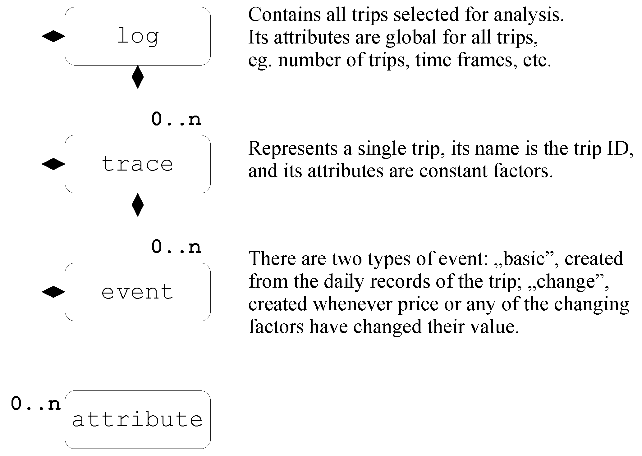
The event log design for trips is based on the eXtensible Event Stream (XES) format [30]. Its main element—the root—is log, and it contains all realized flows of the analyzed process. A log element contains a number of trace elements, each of which is a representation of a single process flow. A trace element consists of a number of event elements, where an event can be understood as a specific activity performed at a given time as part of the single process flow. The XES format allows for adding an unlimited number of attributes at different levels of the tree (for log, trace, and event elements). These attributes allow for adjusting the Event Log syntax to the needs of a specific project. Figure 13 shows the simplified UML diagram of the Event Log with an overview of what trip data have been assigned to the specific elements.

The PM4Py [31] library was used to generate Event Logs and model business processes. This library allows the creation of an object-oriented representation of the event log. Since a lot of data was processed in the project, dedicated methods were implemented that transformed tourist data from the Data Frame directly into Event Log objects, bypassing its XML representation.

This data transformation process takes the longest time; of course, the longer it is, the more data there is to transform. Therefore, before the transformation, the data were pre-filtered and sampled. For example, only those trips where the price changes at least once were selected. Trips with less than 30 days (last minute) and more than 30 days until departure are separated into two Event Logs. When it is known in advance what data are expected in the log, pre-filtering the data and then generating the Event Log is much more efficient than creating a very large Event Log and then filtering it.

4.2. Process Model

Process models can be discovered based on the entire Event Log or filtered by attributes. It allows for analyzing the data at different levels of detail or dividing it into groups in relation to one of the constant factors. Filtering can be conducted on the level of whole traces or individual events.

There are many process mining tools that could be used to analyze the Event Logs. There were mainly four methods used:

1.

Directly-Follows Graph (DFG)—a simple representation of the process models. Each node represents an activity with the frequency of occurrences and the arcs describe the relationship between various activities. The weight of the edges is the number of transitions from one activity to the next. The MAX_NO_EDGES_IN_DIAGRAM parameter allows for adjusting the detail of the graph.

2.

Heuristics Miner—use a representation similar to DFG with frequencies of events and sequences, called a heuristics net. The basic idea is that infrequent paths are omitted from the model. Whether an arc will be added to the model is determined by the dependency value greater than the value of the DEPENDENCY_THRESH parameter.

3.

Transition Matrix (SM)—from the heuristics net object, the activities_occurrences and dfg_matrix can be read. Based on these data, Transition Matrices were calculated. In the matrix cells, there are values corresponding to the problem: what percentage are the situations in which the change of one factor immediately precedes the change of the other factor. The formula is:

$$T{M}_{A,B}=\frac{n\left(A\stackrel{}{\to }B\right)}{n\left(A\right)}·100\%$$

(2)

where:

A, B—activities denoting the change of the factor, e.g., OPEC up

$n\left(A\right)$—number of occurrences of an activity A

$n\left(A\stackrel{}{\to }B\right)$—number of direct transitions from an activity A to B

4.

Cortado Variant Explorer [32] is one of the views generated by the Cortado tool. It clearly presents variants of the occurrence of activities with their actual sequence preserved. This tool also allows for generating process models based on sequences of activities, but in the problem under consideration, these models did not give the expected results.

Using the above-mentioned methods, tourist data were analyzed in many different variants, and thus many models were generated that cannot be discussed in detail in this paper. One changing factor was chosen to demonstrate the process mining example: the barrel of oil price (OPEC). Other Event Log settings are presented in

Table 7. Event Log settings.

offers start day	1 March 2021
Offers end day	30 November 2021
Trips start day	1 March 2021
Trips end day	30 November 2021
Days until departure condition	<30
Traces	8514

. The Event Log was created for one tour operator.

The fuel price change factor is recorded when the absolute value of the difference of the last two prices is greater than 0.5$. The activity “OPEC up” means a fuel price increase and similarly “OPEC down” means a fuel price decrease. The same naming rule has been applied to the trip prices. For trips, every price change is recorded, without any thresholds.

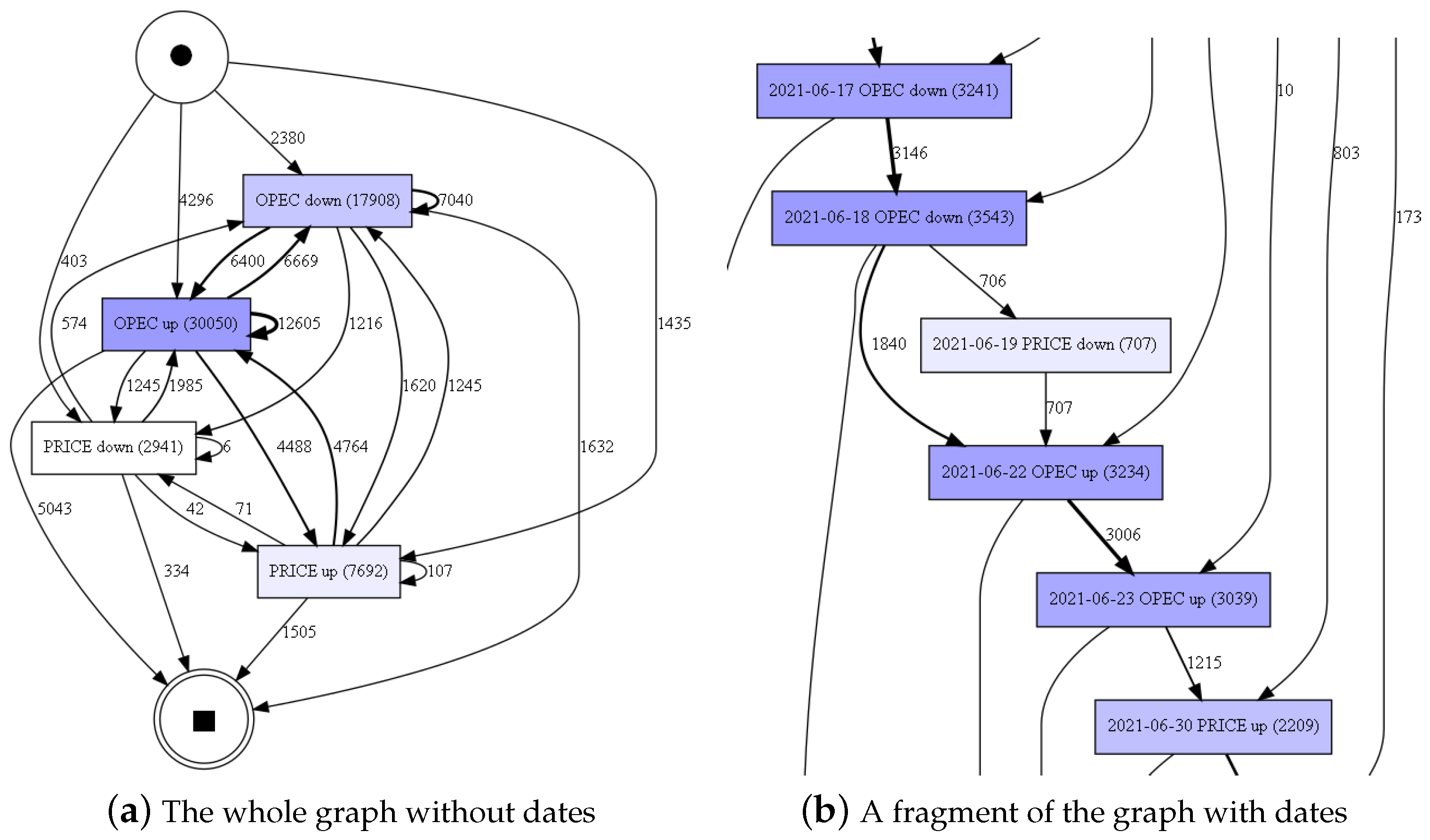
Figure 14 presents two DFGs with different levels of detail. Figure 14 shows the number of occurrences of a given change and the transitions between them. It is quite general, with no dates or individual sequences. It can noticed that the vast majority of trip prices have increased in the last 30 days before departure and considering the relation from OPEC to PRICE, the most numerous transitions are from “OPEC up” to “PRICE up”. This model is used to compute the Transition Matrix shown in

Table 8. TM for relation with OPEC $\stackrel{}{\to }$ PRICE.

A:	OPEC Up	OPEC Down
$A\stackrel{}{\to }$ PRICE up	14.94%	9.05%
$A\stackrel{}{\to }$ PRICE down	4.14%	6.79%

. Figure 14 shows a fragment of DFG with dates. It can be observed that the decline in OPEC prices took place on 17 June and 18 June, while on 19 June, 707 trip prices dropped. On the other hand, on 22 June and on 23 June, the fuel prices increased, while on 30 June, the prices of 1215 trips increased.

Table 8 shows that after the increase in OPEC prices, about 15% of trip prices increased, and this is the greatest relationship. However, also after the decline in OPEC prices, around 9% of the trip prices rose. This situation may be due to the fact that prices are mostly rising 30 days before departure and OPEC is just one of many factors that can influence it. Moreover, the table does not take into account the series of OPEC price changes.

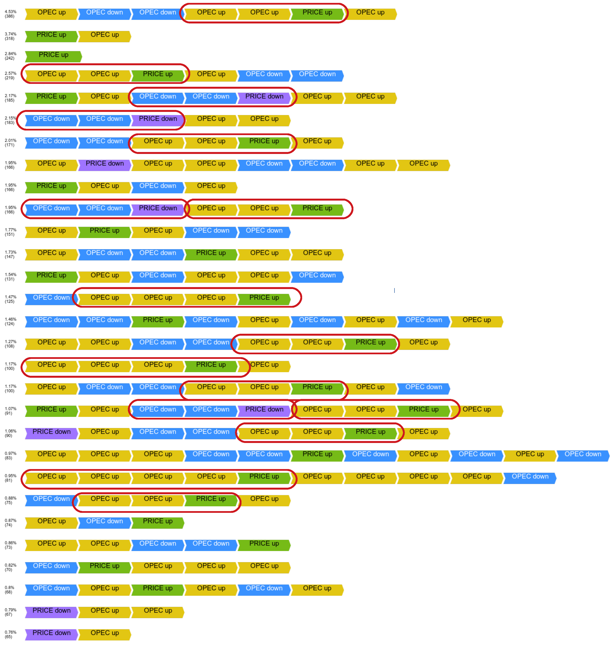
The series of changes can be analyzed, for example, using the Cortado Variant Explorer tool. Figure 15 presents the 29 most common sequences of price changes. A frequent situation (circled in the Figure) is an increase in the trip prices after the series of OPEC price increases and a fall in the trip prices after a series of OPEC price drops. This may indicate that with frequently changing factors, the trend of these changes, not a single change, may contribute to a change in the trip prices.

These types of process mining actions were performed for different factors and filters, allowing many different conclusions to be drawn. However, they are too numerous and detailed to list in this paper. There are, however, a few general conclusions worth mentioning here. Firstly, trip prices generally also increase in the last 30 days before departure—so in most cases, the cheapest trips are at the beginning of the offer (first minute). Prices rarely change and there are some single days on which many prices change, e.g., at the beginning of the month. A series of factor changes show a greater impact than single changes. Economic factors demonstrate a great influence, but they rarely change (e.g., once a month). In Poland, a drop in air temperature affects the increase in the prices of the last minute trips to warm countries.

5. Conclusions

The presented results confirmed that time-varying factors have the greatest impact on changes of trips prices. Among them, currency rates and oil barrel price and their rates of change are the most significant ones. The number of days a trip has been already offered also turned out to be important. However, some constant variables are also worth being taken into account. Among them, the tour distance seems to be essential.

The results of our work is a part of the innovative solutions enabling the effective selection of travel offers by consumers based on information provided by price prediction mechanisms implemented as meta-search engines. Moreover, these solutions enable advanced analysis of historical data for the travel market (i.e., tour operators, travel agents, brokers of tourist offers, and owners of hotels in Poland) available as a Software as a Service. Thanks to these solutions, participants of the tourism market, including primarily smaller entities that do not have their own technological facilities, will be able to compete with large players on the market in terms of pricing policy, more effective distribution of tourism products and services, and revenue management.

The obtained results might be biased by the time data were gathered, which was pandemic. However, the proposed methodology might be applied to any period. Moreover, when more training data are gathered, it is advisable to rerun the implemented procedures to update the results. Feature rankings might change, especially if training data from several years are available.

Several ideas come into mind to try to improve the selection of best predictors in future works. First of all, it is worth taking into account the heterogeneity among trips and across time. Although the tree-based models applied in the presented study are able to partition feature space and make examples follow different decision paths in different regions of the space, there are also other approaches. It is possible to perform data clustering prior to feature selection. Two types of clustering are worth investigating. It may be performed on the basis of expert knowledge, e.g., trips might be grouped depending on the region or on the season. Clustering may be also performed automatically by applying some of the well known algorithms [33,34,35]. After clustering, the data feature selection could be performed separately in each cluster, letting finding different feature subsets be optimal in different areas of the feature space.

Another approach to incorporate some sources of heterogeneity while creating a model was presented in [36], where the authors assumed that individuals living in a particular location have homogeneous preferences. They applied geographically weighted multinomial logit models to estimate preferences over management options for national forest area. In this method, a set of local models together with location weights that incorporate distances between observations and locations was obtained. In this way, it was possible to take into account the fact that the relation between variables varied across space. It is also possible to account not only for the spatial heterogeneity but any other, including unobserved variable heterogeneity, by applying the mixed logit model. In [37], it was even demonstrated that model performance might be improved if the heterogeneity was modeled among cohorts, i.e., groups of individuals sharing common characteristics at a time or experienced a common event, rather than individuals.

Another idea to improve the power of price predictors is to investigate other features not taken into account in this study. One such feature could carry information on some events at the destination location. Obviously, any natural disasters or terrorist threats might reduce interest on a given location. On the other hand, some sport or cultural events may attract more tourist than usual. All of these may have an impact on trip prices. Information on the events should be extracted automatically from some available sources, e.g., Wikipedia Current events or social media platforms. This complex task requires implementing web mining and natural language processing techniques [38,39]. Mining the web could also deliver valuable information on current tourist destination preferences, which should be added as another parameter worth investigating.

A very interesting research could be a thorough investigation of the idea presented in Section 4 and comparing the results generated by two different approaches, i.e., process mining and feature selection.

All efforts made in order to eliminate irrelevant or redundant information would benefit the future system of price prediction, as it may improve the accuracy of the final prediction model. Moreover, it would reduce the time and space complexity of the implemented algorithms, which require training the models on the basis of large volumes of data. Finally, the elimination of some parameters may bring economic benefits during the data collection stage, because of the high costs of gathering and integrating data, both in the sense of time and money.