Abstract
Conflict detection is an essential issue in flying ad hoc networks (FANETs) to ensure the safety of unmanned aerial vehicles (UAVs) during flights. This paper assesses the applicability and utilization of a conflict detection algorithm that sees immediate trajectory as a straight line for short periods with nonlinear mobility models such as Gauss–Markov (GM). First, we use a straight line conflict detection algorithm with two nonlinear mobility models. Then, we perform an extensive simulation study to evaluate the performance. Additionally, we present a comprehensive discussion to tune the collision detection parameters efficiently. Simulation results indicate that an algorithm considering the immediate trajectory as a straight line to predict conflicts between UAVs can be applied with nonlinear mobilities and can provide an acceptable performance measured in false and missed alarms.
1. Introduction
Recently, unmanned aerial vehicles (UAVs), also known as drones, have gained a lot of attention in several fields because of their versatility, autonomous mobility, and fast deployment, alongside line-of-sight link connections between them, which gives a communication advantage. Researchers investigate the multi-UAV systems to employ them in civil and military applications with minimum human involvement. Drones can be used for remote visual inspection [1,2], packages delivery [3], and search and rescue [4] applications, to name a few. It is possible to utilize multiple UAVs to form flying swarms that can be used to create a self-organizing flying ad hoc network (FANET) without the need for a centralized administration or network infrastructure [5]. FANETs have the advantage of possible deployment in critical and risky situations when terrestrial mobile devices cannot operate or when the communication infrastructure is not available or destroyed.
One of the essential concerns when flying drones is ensuring their safety, including detecting and avoiding conflicts and eventual collisions in the shared space. Conflict happens when the distance between two drones becomes less than a specific value, i.e., loss of separation. Therefore, the conflict detection process predicts the loss of separation between the drones. Conflict detection is important to ensure flight safety, as it forecasts potential collisions. Several works in the literature tackled the conflict detection problem, such as [6,7]. These works assume that the drones will move in a straight line. However, the drones do not move in a strictly straight line but they fluctuate throughout the way. Thus, this work aims to study the performance of a conflict detection algorithm that views the immediate trajectories as straight lines for short periods to predict possible conflicts while using nonlinear mobility models. The mobility models are a major factor that affects protocol simulation [8] and play an essential role in the performance evaluation of ad hoc networks [9] as they represent the node movement and how the speed, position, and acceleration vary over time [10]. Testing a protocol with nonrealistic mobility models that not mimic the nodes’ movement well may lead to inaccurate conclusions.
The contribution of this paper is first to integrate a straight line conflict detection algorithm with two nonlinear mobility models, which are known to better emulate drone trajectories and movement. Secondly, we investigate the performance and usability of the detection algorithm with nonlinear mobility models and study the impact of this change on different metrics, such as the number of missed alarms, number of false alarms, and maneuver time.
The rest of this paper is organized as follows. Section 2 introduces UAV mobility models. Section 3 focuses on nonlinear mobility models. Section 4 briefly describes the used conflict detection algorithm. Section 5 presents the performance evaluation for several nonlinear mobility models with the conflict detection algorithm. Section 6 provides the discussion and possible future directions. Finally, Section 7 concludes the paper.
2. Unmanned Aerial Vehicle Mobility Model
FANET is a type of mobile ad hoc network (MANET). MANETs typically use the random waypoint (RWP) mobility model [11]. The RWP chooses the velocity of the node and the direction randomly, and then the mobile node moves to the destination in a straight line. When the node reaches its destination, it pauses and chooses a new destination. Thus, using the RWP, the node is subject to sudden changes in speed and directions and sudden stops. Moreover, with RWP, a node can undergo a turn. Figure 1a shows an example of a path generated using this model. However, the UAVs have aerodynamic and mechanical restrictions that prevent them from performing such turns (illustrated in red circles in Figure 1a) [12]. Obviously, this mobility model is unrealistic for UAVs and may lead to inaccurate results when using simulations to study protocol performance. Additionally, the work in [13] shows that using typical MANET mobility models may produce undesirable trajectories for UAV applications. Different UAV formations and movements directly affect the mobility of multi-UAV systems. To address this issue, FANET mobility models are proposed.
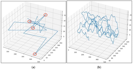
Figure 1.
Sample paths under (a) random waypoint; (b) Gauss–Markov.
3. Nonlinear Mobility Model
3.1. Gauss–Markov Mobility Model
A Gauss–Markov (GM) mobility model is a nonlinear and random model. It was first proposed in [14] and is motivated by the requirement for a closer to reality model in the sense that the UAV will accelerate, deaccelerate, and turn gradually. Thus, the movement (direction and speed) in GM is related to the previous movement through Gaussian equations using average direction and speed of the movement, as well as random Gaussian noise, besides a parameter that controls the degree of the dependency of the previous movement. In that sense, GM is also considered as a temporal dependency model, as the time is divided into slots, and the movement at each time slot depends on the movement of the previous time slot. Thus, the movements are correlated [15]. Figure 1b shows a sample of a trajectory generated by the GM mobility model.
The GM mobility model emulates the real environment for drone communications [16]. The GM was adopted for use in several recent FANET-related studies [16,17,18,19,20].
GM works as follows. In the beginning, each drone will have a specific direction and speed. After that, the direction and speed will be changed at each time period. The new direction () and speed () will depend on the previous direction and speed and will be calculated as follows [21]:
where t is the discrete unit of time; is the tuning parameter which adapt the required level of randomness; and are the previous direction and speed at time ; and are the mean of the direction and speed, respectively; and are the standard deviation of the direction and speed, respectively; and are random variables from Gaussian distribution with mean equal 0 and unit variance.
The x and y are then calculated based on the direction and speed as follows:
where () is the x and y coordinate for the node at tth time interval, and () is the x and y coordinate for the node at time interval.
3.1.1. Gauss–Markov Variables
GM has several adjustable variables. The main tuning parameter is , which controls the level of randomness of the model. Another important parameter is time step, which represents how frequently the new values are calculated, and, additionally, the values of the standard deviation of the speed and direction. In the following, we explain the effect of each of these variables.
Alpha : The variable is the tuning parameter for GM. Setting to a value between 0 and 1 allows us to adjust the degree of the model randomness. When , the model will be predictable and lose all of its randomnesses, and the new direction and velocity will be the same as the previous direction and velocity. Thus, when , the drone moves in a straight line:
On the other hand, when , the model will become memoryless, and the new direction and velocity will depend on the mean and standard deviation values of the direction and velocity and the Gaussian random variables.
Time step: The time step greatly affects the dynamics of GM. As the speed and direction will be fixed until the next time step, choosing a large time step will cause a long period of straight movements.
Standard deviation: The value of the standard deviation for the different variables will directly impact the trajectories as it affects the range of possible change of these variables. A much greater standard deviation than the averages produces different movement patterns than if the value is small. Choosing small values for the standard deviation of the direction will make a small direction change at each step, which leads to smoother turns. On the other hand, choosing large values for the standard deviation of the direction can lead to more significant direction change at each step, which leads to sharper turns.
The same thing applies for the speed; choosing small values for the standard deviation of the speed will make a small speed change at each step. For example, if the average speed equals 3, if we want speed values to be within the interval [2.5–3.5] (approximately), the speed standard deviation should be 0.1, but if we want speed values to be in the interval [2–4] (approximately), the speed standard deviation should be 0.2, and so on.
Thus, the standard deviations need to be set carefully based on the physical characteristics of the UAV.
3.1.2. Boundary Handling
There were several proposals on how the model should behave around the boundaries. Bai and Helmy in [15] proposed a direction change close to the boundaries without specifying how to make that change. In [22], the authors proposed a turn around the boundaries. However, this strategy conflicts with one of the main reasons for proposing this model, which is to avoid sharp turns. Additionally, it will eliminate the temporal dependency feature as the direction is not based on the previous direction.
The works in [23,24] proposed forcing the mobile node away from the edge by changing the average of the direction when the node enters into a specific margin zone. In that way, the node moves away from the boundary progressively toward the center of the area. Figure 2 shows the proposed angle change.
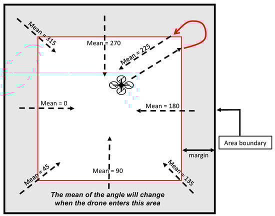
Figure 2.
Change of mean angle near the boundaries.
3.1.3. Extending GM to Three Dimensions
The GM can be extended to 3D in several ways. First, the GM process can be applied to the three dimensions directly, as follows:
The issue with this way is that it is uncharacteristic to model the UAV flight. It is not easy to represent the UAV flight based on the UAV velocity in each direction. UAV flight can be modeled more accurately using a variable for velocity, a variable for direction, and a variable for pitch [25]. In this approach, the velocity and direction are calculated as in the two-dimensional Gauss–Markov, then we add another variable to track the vertical pitch, as follows:
Then, the x, y, and z are calculated as follows:
3.2. Enhanced Gauss–Markov
The work in [12] proposed an enhancement to GM (EGM), trying to limit the sudden stops and sharp turns and guarantee smooth paths around the boundaries. In EGM, a direction deviation is calculated first using the following formula:
where is the direction deviation in previous time . At the beginning it is chosen randomly from the range . The is the mean for direction deviation and it is chosen to be 0. is a random variable from Gaussian distribution with mean equal to zero and variance equal to .
These values are chosen to make the direction deviation small to guarantee gradual direction change, and this will result in more smooth paths.
After that, the new direction is calculated as follows:
The x and y are then calculated based on the speed and direction as follows:
Note that EGM considers two dimensions GM, and the speed is calculated as in the regular GM. Figure 3 shows a path for a UAV using the proposed enhancement implemented in OMNeT++.
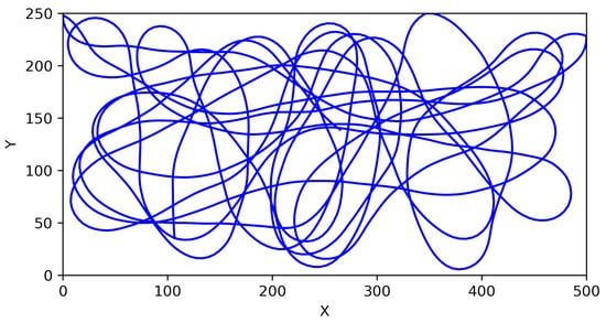
Figure 3.
Drone trajectory in 2D using EGM.
To produce more smooth turns around the boundaries using EGM, the following changes will be applied when the drone approaches any boundary:
- The mean of the direction deviation will be changed to or (depending on the current direction of the UAV).
- Reduction of the variance of the Gaussian distribution to instead of 6.2.
These changes will be applied when the drone moves close to the boundary with a specified distance (margin). The value of this margin should be selected based on the drone’s speed and the value of the time step.
4. Conflict Detection Algorithm (SLIDE)
In [6], the authors proposed a mathematical model for the 3D conflict detection and a new algorithm called “SLIDE”. “SLIDE” is a straight line conflict detection and alerting algorithm for a group of drones to share a common airspace. SLIDE views the drones’ trajectories in the very near future as straight lines and depends only on the position and velocity information which are exchanged periodically between the drones. It does not require a priori knowledge of each drone’s trajectory; the drones can dynamically change their trajectories based on the flight situations and the surrounding environment. Additionally, it does not require any remote visual inspection (RVI) tools such as high-resolution cameras.
To ensure safe navigation in the 3D airspace, each drone is surrounded with a virtual spherical area called the protected zone. The protected zone for any drone should not overlap with any other drone’s protected zone. SLIDE predicts a conflict between two drones if their protected zones overlap at any time (t) within its prediction time (also called look ahead time) . SLIDE is a distributed algorithm; each drone individually uses its state information along with the states received from its neighbor drones to decide whether it is going to lose the safe zone during the prediction period. Each drone periodically sends (in each broadcast cycle ) its state information message, which contains its current position, velocity, and the radius of its protected zone. More specifically, SLIDE works as follows:
- Input: and .
- Output: Whether the drone will encounter conflicts during the , and the timing of the conflicts (if any).
- Process: Each drone broadcast its information periodically every in a STATE message that contains the following:
- −
- Current position;
- −
- Current speed;
- −
- The protected zone radius.
When a drone receives the STATE message, it will calculate if there is a potential conflict during the , assuming that the two drones will continue in a straight line path. Each drone maintains a conflict table to record all information about conflicts, such as the identifiers of conflicting drones and the starting and ending time of the conflict. The start time of a conflict is when the overlap between the protected zones is expected to begin. The end time of a conflict is when the overlap between the protected zones is expected to finish. The conflict times are calculated using the drone’s local time, so there is no need for synchronization between the drone’s clocks.
Back-off time is used to avoid losing STATE messages when several drones try to send simultaneously. Each drone will wait for some random number chosen randomly and uniformly distributed from the interval . The maximal should be selected based on the network density. For high density, should be increased to avoid simultaneous broadcasts.
5. Performance Evaluation
SLIDE is implemented using the OMNeT++ simulator [26]. A comprehensive performance evaluation for SLIDE using RWP mobility can be found in [6]. The aim of this paper is to validate SLIDE and its usability with different mobility models, or, more specifically, with nonlinear mobility models (GM and EGM).
5.1. Simulation Setup
In the simulation setup, we consider the specifications of small drones, specifically Parrot AR.Drone [27]. The dimensions of AR.Drone are 51.7 cm × 51.7 cm, equipped with an 802.11 radio, and it can fly with its maximal speed of 5 m/s for approximately 12 min.
In each scenario, we consider the following:
- N drones flying for 10 min in a confined space with the dimensions 500 m × 400 m × 30 m.
- All drones have the same protected zone radius R.
- All drones have the same communication range .
- The drones use IEEE 802.11 protocol to communicate with each other directly.
- The maximal back-off time is set to 1 s.
- The environment is static, with no obstacles except the other drones and the boundary limits.
Every scenario is repeated 30 times. Table 1 contains the considered parameters for the simulation environment and Table 2 contains the considered parameters for GM and EGM. Figure 4 and Figure 5 show samples of the paths generated using these parameters.

Table 1.
Simulation parameters for the environment.
Table 2.
Simulation parameters for GM and EGM.
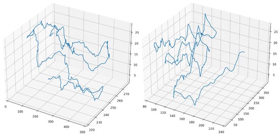
Figure 4.
Samples of the generated paths using GM.
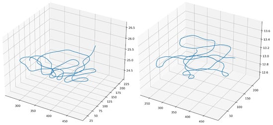
Figure 5.
Samples of the generated paths using EGM.
5.2. Slide Behavior with Different Mobility Models
In this section, we investigate the performance of SLIDE after changing the mobility model. We compare the performance of SLIDE under three different mobility models. First, we study the effect of the simulation parameters (broadcast cycle , velocity v, communication range , look ahead time , and the protected zone R). Second, we compare the scalability. Finally, we study the effect of the mobility model parameters.
5.2.1. Effect of Simulation Parameters
Figure 6 shows the number of missed alarms using various broadcast cycles and velocities for SLIDE using GM, EGM, and RWP, respectively. The number of drones N is 40, the protected zone R is 1 m, and the look ahead time is 8 s.
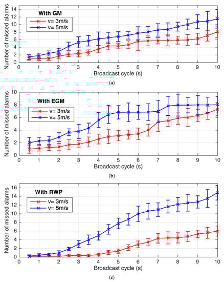
Figure 6.
Average missed alarms under different using (a) GM; (b) EGM; (c) RWP.
As expected, increasing the broadcast cycle leads to an increase in missed alarms. With the RWP, the broadcast cycle should be less than to avoid missed alarms, thus, less than 3.8 s when the speed equals 3 s and 2.3 s when the speed equals 5 s. With the nonlinear mobilities, as there is a randomness factor, the drone’s next position may differ from the expected position. For EGM, the direction standard deviation is 2.49, which will make the next angle vary approximately by the range (the range is different around the boundary). For the GM, we set the angle standard deviation to 10, so the next angle varies approximately by the range . For instance, when speed equals 3 m/s and the time step equals 0.5, if the angle changes by 4.5 degrees, the distance between the expected and the actual location will be around 15 cm. These values have a small but cumulative effect on the drone’s path, so GM and EGM performance are close for lower broadcast cycles and speed. However, as the broadcast cycle and speed increase, we can see that the EGM outperforms GM because the angle change is less using EGM. Besides that, EGM produced more smoothed paths around the borders; Figure 7 shows examples of how GM and EGM behave around borders.
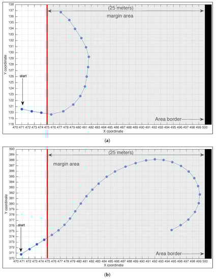
Figure 7.
Samples of the paths around the boundary using (a) GM; (b) EGM.
Notably, the number of missed alarms for higher broadcast cycles is lower than that of the RWP. It is because the number of actual collisions is lower using GM and EGM. A possible reason for this is their movement pattern. Several works in the literature compared RWP with GM and concluded that GM leads to uneven node distribution, and they became more isolated for some time [28]. Figure 8 shows the movement pattern for three nodes with RWP and GM.
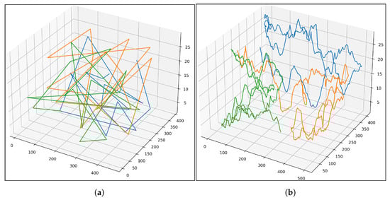
Figure 8.
Traveling patterns of nodes with (a) RWP; (b) GM.
Figure 9 shows the number of missed alarms using different communication ranges and velocities for SLIDE using RWP, GM, and EGM, respectively. The considered broadcast cycle is 2, protected zone R is 1, and the look ahead is 8. These figures show clearly that the number of missed alarms decreases when the communication range increases. The algorithm will receive additional state information with larger communication ranges, enhancing the general performance.
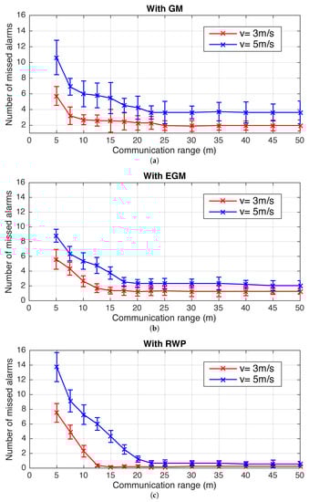
Figure 9.
Average missed alarms under different using (a) GM; (b) EGM; (c) RWP.
Figure 10 shows the impact of the look ahead time , communication range , and protected zone radius R on the number of false alarms. The figures clarify that increasing , R, and lead to an increase in false alarms. For a particular R and , when increases, false alarms increase until they reach some maximum value. For instance, with RWP, when R = 2.5 and = 25, there were around two false alarms when = 2 s, and 4.9 false alarms when = 10 s, then the false alarms stabilize at this point. Similar behavior appears with GM and EGM but with larger false alarm values. This indicates that the prediction performance depends directly on the accuracy of the expected paths. The more distant in advance a prediction is, the less likely it is that such a prediction will be accurate because unexpected turning maneuvers are more likely to occur. SLIDE is a straight line conflict detection algorithm, yet it can provide acceptable performance for some small look ahead times with nonlinear mobilities such as GM and EGM. In fact, when the is 25, the benefit of a large look ahead is reduced, as this communication range gives us around 4 s on average for maneuvering even with RWP (Figure 11c).
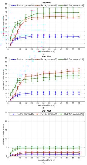
Figure 10.
Number of false alarms under different , , and R using (a) GM; (b) EGM; (c) RWP.
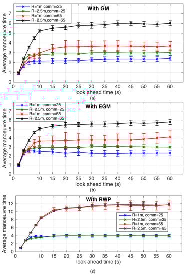
Figure 11.
Average maneuver time under different , , and R using (a) GM; (b) EGM; (c) RWP.
If the is 25 m and the speed is 3 m/s, and assuming two drones enter each other’s range and head to each other, this will give 8 s until the collision. Such conflict cannot be predicted before that. Therefore, a minimum of 8 s for look ahead is required in this case ( = 25 and speed = 3) to detect such conflicts. However, we should avoid larger look ahead values with nonlinear mobility as they will negatively impact undetected conflicts and false alarms. Using GM and EGM, the drones will change their heading at each step (the considered time step (update interval) for both GM and EGM is 0.5 s), and the actual position in the near future may differ from the expected position by SLIDE. Figure 12 shows a sample of a GM path and compares it with the expected straight line path for 60 s. The distance between them reaches 7 m after 39 s.
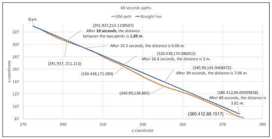
Figure 12.
Sample of GM path and the expected straight line path for 60 s.
The same applies to the EGM, with the difference that with EGM, in the beginning, the difference between the paths is less than the GM case, then the drone starts heading in a completely different direction (Figure 13).
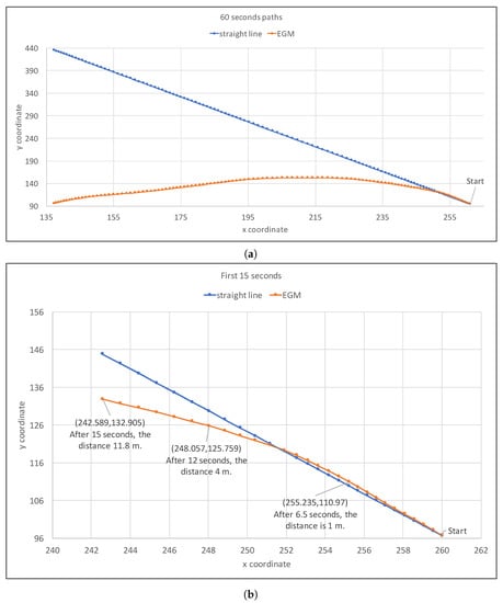
Figure 13.
Sample of EGM path and the expected straight line path for (a) 60 s; (b) 15 s.
Furthermore, for a specific and , the false alarms will rise by increasing the protected zone radius R from 1 m to m. For example, with GM, when s and m, the number of false alarms is 12 when m and becomes 30 when R is increased to . We see the same behavior with the EGM; the false alarms increased from around 10 to 26. The reason for this rise is that the radius of the protected zone will increase the number of actual conflicts. For instance, with GM, the number of actual conflicts is 8 with a protected zone radius of 1 m and 60 conflicts with a protected zone radius of m. This rise in the number of actual conflicts will increase the number of detected conflicts, and accordingly, the probability of false alarms will increase. In the same way, for a fixed and R, the number of false alarms will rise by increasing the communication range from 25 m to 65 m because each drone will have more nearby drones to consider, which will also increase the possibility of false alarms.
Figure 11 shows the average maneuver time and its relation with , , and R. For both GM and EGM, the maneuver time increases by increasing , , and R until it converges at some maximum value.
From the analysis of Figure 10 and Figure 11, we can conclude that the selections of and are a trade-off between the disturbance alarms and higher safety margin. Raising or will raise the maneuvering time but at the expense of raising the false alarms. On the other hand, lowering or will reduce the false alarms at the expense of reducing the maneuvering time, which may become not enough for avoidance maneuver.
Table 3 shows the number of false alarms under different airspace dimensions. We consider two speeds, and , and two look ahead times, and . The broadcast cycle is set to 2 s. We can see that the false alarms for all mobility models reduce as the airspace expands and the speed dropps. In larger airspaces, the drones will move in straight lines more frequently and have fewer turns, whereas in smaller airspaces and with faster speed, the drone will reach the boundaries faster, and the change of direction will be larger. Thus, to avoid large false alarms in smaller airspaces, we should use smaller .
Table 3.
Average false alarms with different airspace dimensions.
5.2.2. SLIDE Scalability
Table 4 displays the number of actual conflicts, missed and false alarms, the probability of missed and false alarms, and the average maneuver time under a different number of drones. As the experiments from the previous section show that the performance of SLIDE is affected directly by the tuning parameters and , their values should be carefully selected to ensure acceptable performance for conflict detection. The considered value of is 2 s, and is 8 s.
Table 4.
SLIDE scalability.
Table 4 shows that, regardless of the growth of the number of drones from 40 to 120 and the growth of the number of actual conflicts from around 8 to 80 s, the probability of missed and false alarms remains almost constant for all mobility models. The same applies to the average maneuver times, in which it stays stable. For instance, with GM, SLIDE maintains a stable and low probability of missed alarms (around 0.2), an acceptable and stable probability of false alarms (around 1.5), and a stable average maneuver time of approximately 2 s. With EGM, also, SLIDE keeps a stable and lower probability of missed alarms (around 0.15), an acceptable and stable probability of false alarms (around 1.5), and a steady average maneuver time of approximately 2.5 s. Indeed, Table 4 shows that SLIDE is still scalable to an increasing number of drones even with nonlinear mobilities.
5.2.3. Effect of Mobility Model Parameters
The parameters of GM give the flexibility to adjust the model to be suitable for different movement patterns. Thus, they need to be chosen based on the physical characteristics of the UAV. In this section, we perform several experiments to evaluate the performance of SLIDE when changing the mobility model parameters. The considered is 2 s, is 8 s, and speed is 3 m/s.
First, we test the model with different time step values. Figure 14 shows the number of missed alarms under the following time steps (0.1 s, 0.25 s, 0.5 s, 0.75 s, 1 s, and 1.5 s). The figure shows that when the time step increases, the number of missed alarms decreases. With a larger time step, the drone will move with the same speed and direction for a longer period. In SLIDE, the drones periodically send their current locations and velocities. When a drone receives this information, it calculates if any possible conflict will occur in the near future. This calculation assumes that each drone will continue in the same direction, thus in a straight line. However, using GM, the direction will change randomly at each time step. For example, if the broadcast cycle is 0.5 s and the time step is 0.1 s, each drone will change its heading four times before sending its information again. On the other hand, if the broadcast cycle is 0.5 s and the time step is 1.5 s, the drones will change their heading once after sending their information so that the location will be accurate for around 1 s.
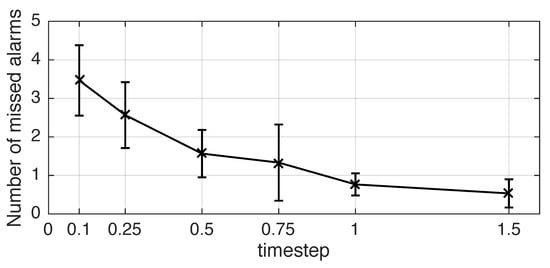
Figure 14.
Impact of time step on the number of missed alarms.
To understand how changing the standard deviation affects SLIDE’s performance, we vary the standard deviation of the angle, pitch, and speed in Figure 15a–c, respectively. For instance, Figure 15a depicts the result of changing the standard deviation of the angle from 0.5 to 20. The average number of missed alarms remains constant for the standard deviation from 0.5 to 7.5, then increases incrementally. Changing the angle’s standard deviation controls the direction change in each step, then the node will move in the new direction until the next time step. We can also see a similar effect from changing the pitch standard deviation in Figure 15b. We vary the standard deviation of the pitch from 0.1 to 20. The average number of missed alarms remains constant for the standard deviation from 0.1 to 7.5, then increases incrementally. Changing the standard deviation of the pitch controls how high (or low) the drone can move far from the initial altitude. With higher values for the pitch standard deviation, the drone altitude difference is more.
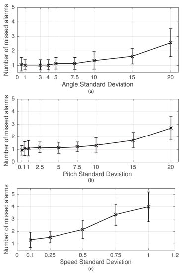
Figure 15.
Impact of the standard deviation on the number of missed alarms: (a) angle SD; (b) pitch SD; (c) speed SD.
Figure 15c shows the result of changing the standard deviation of the speed from 0.1 to 1. As with the other standard deviations (angle and pitch), the number of missed alarms increases when the standard deviation increases. However, the algorithm is more sensitive to the speed change than the angle or altitude change. For instance, if the selected speed is 3, and the speed standard deviation is 0.5, the speed can reach 5 m/s. As the drone will move in the new direction for a longer distance, the errors will be accumulated much faster.
6. Discussion and Future Work
There are two main reasons for missed alarms using SLIDE: the first is when the messages are not received. The second is because a conflict will be considered as detected only if the conflict’s position and timing are both correct.
- Losing messages: This has more effect when using GM and EGM (or nonlinear) mobility, as the drone’s direction will change more frequently. However, when using RWP, if a message is received, the drone will stay on the same line for some time, so all (or most) conflicts within the look ahead time can be detected, even if the next message is lost. In other words, there are several chances to detect a conflict, especially with small broadcast cycles. Thus, to avoid losing messages or to minimize its effect, the broadcast cycle should be small, and the density of the drones must be suitable for the environment.
- Conflict time/place: SLIDE will not only predict if there is a conflict or not, but it also specifies the conflict interval, i.e., the time of the beginning of the conflict and the time of the end of the conflict. Using GM and EGM, the drones will change their heading at each step (the considered update interval is 0.5 s), and the actual position in the near future may differ from the predicted position by SLIDE. As an example, in one of the scenarios, a conflict between two drones happened at the time 20.5; SLIDE using GM predicts that the conflict will start at the time 21.1, the difference here is 0.6 s, and the algorithm considers this as undetected conflict (for the difference in timing). To minimize the errors in calculating the time and place, the changes in the angle and speed should not be large. For the experiments in Section 5.2.1, we tested the algorithm with high values for the standard deviations to present the general performance of the algorithm. The experiments in Section 5.2.3 show that the performance will improve when the standard deviations decrease.
In summary, to eliminate or minimize the missed alarms, SLIDE parameters, along with the mobility model parameters, need to be adjusted, and the environment needs to be studied carefully. From the experiments, SLIDE is expected to provide acceptable performance in predicting conflicts in large spaces with lower drone speed. Considering all these factors, SLIDE provides acceptable performance in predicting conflicts with nonlinear mobilities, with one missed alarm, on average, in most scenarios for 40 drones when the broadcast cycle is 2 or less. Thus, if we guarantee that all messages arrive and bound the angle change to some upper and lower limits, the errors in calculations will be reduced. This point can be further investigated in the future. Another interesting direction to explore is to study the impact of using 4G communication technology instead of the IEEE 802.11 protocol. From the provided experiments and analysis, it is expected that changing the communication model will directly impact the performance.
7. Conclusions
This paper investigates the performance and usability of a straight line conflict detection algorithm with nonlinear mobility models. First, we present two implementations of nonlinear mobility models for drones. Namely, Gauss–Markov and enhanced Gauss–Markov (EGM) [12]. Then, we compare the results using these nonlinear mobility models with the performance under a straight line mobility model (particularly, RWP). The results show that the straight line conflict detection algorithm can provide scalable and acceptable performance if the parameters are tuned carefully based on the environment for each mobility model.
Author Contributions
Conceptualization, M.A. and A.B.; methodology, M.A. and A.B.; software, M.A. and A.B.; formal analysis, M.A. and A.B.; investigation, M.A.; data curation, M.A.; writing—original draft preparation, M.A.; writing—review and editing, M.A. and A.B.; visualization, A.B.; supervision, A.B.; project administration, A.B.; All authors have read and agreed to the published version of the manuscript.
Funding
This research was funded by Deanship of Scientific Research at King Saud University.
Institutional Review Board Statement
Not applicable.
Informed Consent Statement
Not applicable.
Data Availability Statement
Not applicable.
Acknowledgments
The authors would like to thank the Deanship of Scientific Research at King Saud University for funding and supporting this research through the initiative of DSR Graduate Students Research Support (GSR).
Conflicts of Interest
The authors declare no conflict of interest.
References
- Balsi, M.; Moroni, M.; Chiarabini, V.; Tanda, G. High-Resolution Aerial Detection of Marine Plastic Litter by Hyperspectral Sensing. Remote Sens. 2021, 13, 1557. [Google Scholar] [CrossRef]
- Filkin, T.; Sliusar, N.; Ritzkowski, M.; Huber-Humer, M. Unmanned Aerial Vehicles for Operational Monitoring of Landfills. Drones 2021, 5, 125. [Google Scholar] [CrossRef]
- Saponi, M.; Borboni, A.; Adamini, R.; Faglia, R.; Amici, C. Embedded Payload Solutions in UAVs for Medium and Small Package Delivery. Machines 2022, 10, 737. [Google Scholar] [CrossRef]
- Ho, Y.H.; Tsai, Y.J. Open Collaborative Platform for Multi-Drones to Support Search and Rescue Operations. Drones 2022, 6, 132. [Google Scholar] [CrossRef]
- Pasandideh, F.; da Costa, J.P.J.; Kunst, R.; Islam, N.; Hardjawana, W.; Pignaton de Freitas, E. A Review of Flying Ad Hoc Networks: Key Characteristics, Applications, and Wireless Technologies. Remote Sens. 2022, 14, 4459. [Google Scholar] [CrossRef]
- Mahjri, I.; Dhraief, A.; Belghith, A.; AlMogren, A.S. SLIDE: A Straight Line Conflict Detection and Alerting Algorithm for Multiple Unmanned Aerial Vehicles. IEEE Trans. Mob. Comput. 2018, 17, 1190–1203. [Google Scholar] [CrossRef]
- Wan, Y.; Tang, J.; Lao, S. Distributed Conflict-Detection and Resolution Algorithm for UAV Swarms Based on Consensus Algorithm and Strategy Coordination. IEEE Access 2019, 7, 100552–100566. [Google Scholar] [CrossRef]
- Yassein, M.B.; Alhuda, N. Flying ad-hoc networks: Routing protocols, mobility models, issues. Int. J. Adv. Comput. Sci. Appl. (IJACSA) 2016, 7. [Google Scholar] [CrossRef]
- Camp, T.; Boleng, J.; Davies, V. A survey of mobility models for ad hoc network research. Wirel. Commun. Mob. Comput. 2002, 2, 483–502. [Google Scholar] [CrossRef]
- Wheeb, A.H.; Nordin, R.; Samah, A.A.; Alsharif, M.H.; Khan, M.A. Topology-Based Routing Protocols and Mobility Models for Flying Ad Hoc Networks: A Contemporary Review and Future Research Directions. Drones 2022, 6, 9. [Google Scholar] [CrossRef]
- Brown, T.X.; Doshi, S.; Jadhav, S.; Himmelstein, J. Test Bed for a Wireless Network on Small UAVs. In Proceedings of the AIAA 3rd “Unmanned Unlimited” Technical Conference, Workshop and Exhibit, Chicago, IL, USA, 20–23 September 2004; pp. 20–23. [Google Scholar]
- Biomo, J.M.M.; Kunz, T.; St-Hilaire, M. An enhanced Gauss-Markov mobility model for simulations of unmanned aerial ad hoc networks. In Proceedings of the 2014 7th IFIP Wireless and Mobile Networking Conference (WMNC), Vilamoura, Portugal, 20–22 May 2014; pp. 1–8. [Google Scholar]
- Kuiper, E.; Nadjm-Tehrani, S. Mobility models for UAV group reconnaissance applications. In Proceedings of the 2006 International Conference on Wireless and Mobile Communications (ICWMC’06), Bucharest, Romania, 29–31 July 2006; p. 33. [Google Scholar]
- Liang, B.; Haas, Z.J. Predictive distance-based mobility management for PCS networks. In Proceedings of the IEEE INFOCOM’99. Conference on Computer Communications. Proceedings. Eighteenth Annual Joint Conference of the IEEE Computer and Communications Societies. The Future is Now (Cat. No. 99CH36320), New York, NY, USA, 21–25 March 1999; Volume 3, pp. 1377–1384. [Google Scholar]
- Bai, F.; Helmy, A. A survey of mobility models. Wirel. Adhoc Netw. Univ. South. Calif. USA 2004, 206, 147. [Google Scholar]
- Li, Y.; Wang, W.; Gao, H.; Wu, Y.; Su, M.; Wang, J.; Liu, Y. Air-to-ground 3D channel modeling for UAV based on Gauss-Markov mobile model. AEU—Int. J. Electron. Commun. 2020, 114, 152995. [Google Scholar] [CrossRef]
- Jo, Y.i.; Lee, S.; Kim, K.H. Overlap Avoidance of Mobility Models for Multi-UAVs Reconnaissance. Appl. Sci. 2020, 10, 4051. [Google Scholar] [CrossRef]
- Anjum, M.N.; Wang, H. Mobility Modeling and Stochastic Property Analysis of Airborne Network. IEEE Trans. Netw. Sci. Eng. 2020, 7, 1282–1294. [Google Scholar] [CrossRef]
- Chen, Y.J.; Liao, K.M.; Ku, M.L.; Tso, F.P.; Chen, G.Y. Multi-Agent Reinforcement Learning Based 3D Trajectory Design in Aerial-Terrestrial Wireless Caching Networks. IEEE Trans. Veh. Technol. 2021, 70, 8201–8215. [Google Scholar] [CrossRef]
- Korneev, D.A.; Leonov, A.V.; Litvinov, G.A. Estimation of Mini-UAVs Network Parameters for Search and Rescue Operation Scenario with Gauss-Markov Mobility Model. In Proceedings of the 2018 Systems of Signal Synchronization, Generating and Processing in Telecommunications (SYNCHROINFO), Minsk, Belarus, 4–5 July 2018; pp. 1–7. [Google Scholar] [CrossRef]
- Roy, R.R. Random Gauss–Markov Mobility. In Handbook of Mobile Ad Hoc Networks for Mobility Models; Springer: Boston, MA, USA, 2011; pp. 311–344. [Google Scholar] [CrossRef]
- Amoussou, G.; Mahanna, H.; Zblgnlew, D.; Kadoch, M. An OpNet implementation of Gauss-Markov mobility model and integration of link prediction algorithm in DSR protocol: A cross-layer approach. In Proceedings of the OPNETWORK 2005, Washington, DC, USA, 12–14 October 2005; pp. 22–26. [Google Scholar]
- Tolety, V. Load Reduction in Ad Hoc Networks Using Mobile Servers. Master’s Thesis, Colorado School of Mines, Golden, CO, USA, 1999. [Google Scholar]
- Alenazi, M.; Sahin, C.; Sterbenz, J.P. Design Improvement and Implementation of 3D Gauss-Markov Mobility Model; Technical Report; Air Force Test Center: Edwards Air Force Base, CA, USA, 2013. [Google Scholar]
- Rohrer, J.P.; Çetinkaya, E.K.; Narra, H.; Broyles, D.; Peters, K.; Sterbenz, J.P.G. AeroRP performance in highly-dynamic airborne networks using 3D Gauss-Markov mobility model. In Proceedings of the 2011-MILCOM 2011 Military Communications Conference, Baltimore, MD, USA, 7–10 November 2011; pp. 834–841. [Google Scholar] [CrossRef]
- Varga, A. The omnet++ discrete event simulation system. In Proceedings of the ESM’01, Prague, Czech Republic, 6–9 June 2001. [Google Scholar]
- Krajník, T.; Vonásek, V.; Fišer, D.; Faigl, J. AR-Drone as a Platform for Robotic Research and Education. In Proceedings of the Research and Education in Robotics-EUROBOT 2011, Prague, Czech Republic, 15–17 June 2011; Obdržálek, D., Gottscheber, A., Eds.; Springer: Berlin/Heidelberg, Germany, 2011; pp. 172–186. [Google Scholar]
- Peters, K.J. Design and Performance Analysis of a Geographic Routing Protocol for Highly Dynamic MANETs. Ph.D. Thesis, University of Kansas, Lawrence, KS, USA, 2010. [Google Scholar]
Publisher’s Note: MDPI stays neutral with regard to jurisdictional claims in published maps and institutional affiliations. |
© 2022 by the authors. Licensee MDPI, Basel, Switzerland. This article is an open access article distributed under the terms and conditions of the Creative Commons Attribution (CC BY) license (https://creativecommons.org/licenses/by/4.0/).