Article

ConDPC: Data Connectivity-Based Density Peak Clustering

1
College of Computer and Information, Hohai University, Nanjing 211100, China
2
School of Information Engineering, Jiangsu Maritime Institute, Nanjing 211199, China
*
Author to whom correspondence should be addressed.
Appl. Sci. 2022, 12(24), 12812; https://doi.org/10.3390/app122412812
Submission received: 3 October 2022 / Revised: 7 December 2022 / Accepted: 8 December 2022 / Published: 13 December 2022
(This article belongs to the Section Computing and Artificial Intelligence)

Abstract

:
As a relatively novel density-based clustering algorithm, Density peak clustering (DPC) has been widely studied in recent years. DPC sorts all points in descending order of local density and finds neighbors for each point in turn to assign all points to the appropriate clusters. The algorithm is simple and effective but has some limitations in applicable scenarios. If the density difference between clusters is large or the data distribution is in a nested structure, the clustering effect of this algorithm is poor. This study incorporates the idea of connectivity into the original algorithm and proposes an improved density peak clustering algorithm ConDPC. ConDPC modifies the strategy of obtaining clustering center points and assigning neighbors and improves the clustering accuracy of the original density peak clustering algorithm. In this study, clustering comparison experiments were conducted on synthetic data sets and real-world data sets. The compared algorithms include original DPC, DBSCAN, K-means and two improved algorithms over DPC. The comparison results prove the effectiveness of ConDPC.

1. Introduction

Clustering aims at partitioning a collection of objects into different subgroups [1]. Objects are grouped according to their similarity, so the objects in the same subgroup are highly similar [2]. Clustering has been applied in wide areas such as pattern recognition, community detection, image segmentation, trajectory analysis, fault diagnosis, and so on [3,4,5,6,7].
The density-based clustering algorithm is a kind of classical clustering algorithm [8,9,10,11]. Density-based clustering methods can discover clusters of various shapes and sizes [12]. DBSCAN [8] is the most typical representative algorithm in this kind of method. It proposes concepts such as density-reachable to construct densely connected clusters. However, when clusters are distributed in markedly various densities, DBSCAN may obtain bad clustering results. DPC [13] is a relatively novel density-based clustering algorithm, which can obtain the cluster centers semi-automatically with the help of decision graphs. However, when the DPC algorithm deals with data with large density differences or manifold structures, it is easy to produce wrong cluster centers or wrong neighbor assignments.
Based on the DPC algorithm, many scholars have proposed improved algorithms [14,15,16,17,18,19,20]. Du et al. [14] proposed two KNN-based clustering algorithms and incorporated PCA into them. Xie et al. [15] modified the calculation method of local density and the neighbor assignment mechanism. Abdulrahman et al. [16] constructed cluster backbones to better distinguish different clusters. The above algorithms use KNN to calculate the local density, but the clustering error problem of large density difference and nested structure has not been solved. Du et al. [17] proposed a density-adaptive distance calculation method to solve the problem of poor clustering in manifold structure, but the time complexity of the algorithm is high. Wang et al. [18] proposed multi-center clustering based on a hierarchical approach to solve the problem of poor multi-center structure identification. However, the algorithm has four input parameters which make the algorithm difficult to control.
This study integrates connectivity into the original DPC algorithm to improve the clustering effect. The primary contributions of this study are as follows.
(1)
Constructing connected groups based on the idea of connectivity. Points in the same group are connectable to each other, whereas points in different groups are not.
(2)
Adjusting the calculation method of neighbor distance based on the idea of connectivity to improve the accuracy of determining the cluster center.
(3)
Adjusting the neighbor allocation strategy based on the idea of connectivity to improve the accuracy of clustering.
The rest of this paper is organized as follows. We provide an overview of the DPC algorithm in Section 2. Section 3 explains the detailed steps of the proposed algorithm ConDPC. In Section 4, experiments are conducted on synthetic and real-world datasets. Conclusions are presented last.

2. Original Algorithm

DPC algorithm was proposed by Rodriguez et al. in 2014 [13]. The algorithm is based on the assumption that the local densities of cluster centers are high, and different centers are far apart.
Rodriguez et al. [13] obtained two intermediate results for each point in the data set, which were used for the subsequent judgment of density clustering centers and neighbor assignment. Taking point i as an example, the two results are: (1) Local density ρ of point i ; (2) The minimum distance between point i and the points of greater local density than it (For the convenience of description, this distance is called the neighbor distance in the following text).
The authors provided a local density definition based on a Gaussian kernel which is used in our study. The definition is as follows:
ρ i = i j exp ( ( d i j d c ) 2 )
where d i j is the Euclidean distance between points i and j and d c is a given cut-off distance.
The set of points with a density greater than this point can be defined as follows:
N i = { x j X | ρ i < ρ j }
For the convenience of subsequent descriptions, we call the points in N i the big neighbors of point i .
For point i , the nearest point with a local density greater than it is its neighbor. Then, the neighbor distance is defined as follows [21]:
δ i = min ( d i ( N i ) ) ,     N i   i s   n o t   n u l l max ( δ ) ,             o t h e r w i s e
With the help of local density and neighbor distance, the paper leads to the definition of γ as follows:
γ i = ρ i * δ i
The larger the γ value, the more likely the corresponding point is to be the cluster center point. That is to say, the point with a larger local density and neighbor distance value is more likely to be selected as the cluster center point.
Taking ρ as the x-axis and δ as the y-axis to draw the decision graph, the points with a higher γ value can be intuitively found, thus providing strong support for the selection of clustering centers.
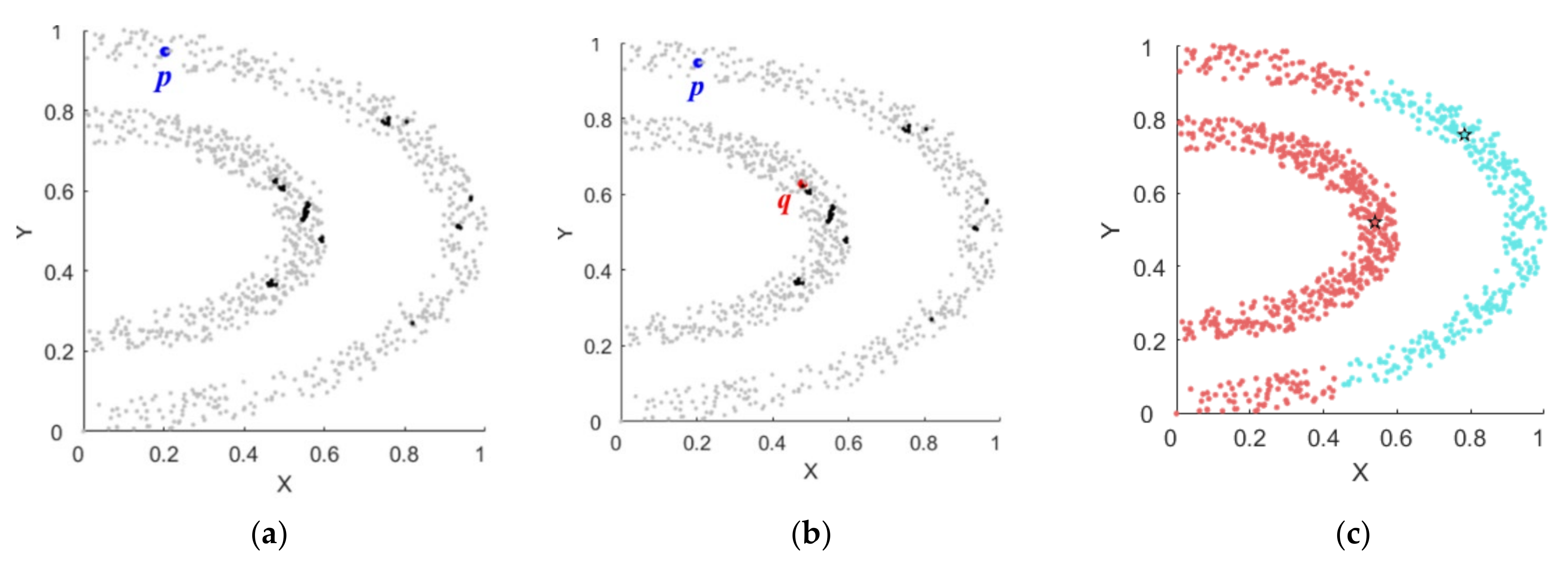
It can be concluded from Formula (1) that the calculation method of local density is the same for each point, that is, the case of large density difference is not considered. This can lead to incorrect cluster center selection. As shown in Figure 1, when the density difference is large, the DPC algorithm may find multiple center points in the group with higher density, while no center points are found in the group with lower density. The two larger dots (marked in red and turquoise) in Figure 1a,b represent the clustering centers selected by the DPC algorithm. In all of the following clustering result figures, the cluster centers are labeled with star shapes. The different clusters produced by the clustering algorithms are distinguished by different colors.
From Formula (3), it can be concluded that the calculation of delta is based on the Euclidean distance. This calculation does not take into account data with manifold structures. This may lead to poor accuracy in neighbor selection. Figure 2 shows the neighbor selection of point p in the external cluster on the Halfkernal dataset. As shown in Figure 2a, the blue point p has several big neighbors (the points marked in black with greater densities than p ). As shown in Figure 2b, the blue point p selects the nearest point q among all the big neighbors as its neighbor. This kind of neighbor selection error leads to the inaccurate assignment of points to the cluster to which they belong. The clustering result is shown in Figure 2c.
To sum up, the DPC algorithm does not consider the density difference and the distance calculation problem caused by the manifold structure, which may lead to the wrong selection of clustering centers or neighbors. In this study, data connectivity is integrated into the original algorithm to solve the above problems.

3. Proposed Algorithm

Drawing on the idea of connectivity, we propose the algorithm ConDPC to improve the accuracy of the DPC algorithm in specific scenarios, such as data distribution with large differences in density or manifold structure.

3.1. Basic Definitions

This section defines the relevant concepts of connectivity.
Definition 1. 
(directly connectable points)
Points i and j are directly connectable to each other if d i j d c , where d c is a given cut-off distance.
The set of points directly connectable to point i is defined as follows:
D N e i s ( i ) = { x j X | d i j d c }
Definition 2. 
(connectable points)
Points i and j are connectable to each other if there is a chain of points p 1   , ,   p n , p 1 = i , p n = j where p k + 1 is directly connectable to p k . This can be marked as r i j = 1 .
Then, the set of points connectable to point i is defined as follows:
L i n k N e i s ( i ) = { x j X | r i j = 1 }
The set of points connectable to point i with a greater density can be defined as follows:
N l i n k i = { x j X | ρ i < ρ j   a n d   x j L i n k N e i s ( i ) }
Definition 3. 
(connected group)
A group is connected when any two points in the group are connectable to each other.

3.2. Steps of the Proposed Algorithm

The algorithm can be divided into three steps: (1) determine the connectivity relationship between points; (2) calculate δ value according to the connectivity relationship and assign neighbors; (3) determine cluster centers and assign labels.
Step 1: Determine the connectivity relationship between points.
In the first step, connected groups are constructed to determine the connectivity between points. The algorithm idea is summarized, as shown in Algorithm 1.
Algorithm 1 Calculate connected groups
Input: input dataset; cutoff distance
Output: connected groups
1.  Mark all points as ungrouped;
2.  For each point i that has not been grouped
3.      Create a new group G, mark point i as grouped in G, and add its directly connectable point set D N e i s ( i ) to G;
4.      For each point j in G that has not been grouped
5.          Mark point j as grouped in G, and add its directly connectable point set D N e i s ( j ) to G;
6.        End For
7.  End For
8.  Return connected groups;
Step 2: Calculate δ and neighbor assignment based on connectivity.
The original algorithm does not consider the connectivity relationship between two points, directly calculates the distance between point i and its big neighbors, selects the minimum value as the δ value of i , and takes point j with the minimum distance as the neighbor of point i .
According to the connectivity relation, the proposed algorithm considers whether two points are connectable to each other when choosing neighbors and calculating neighbor distance.
If there is a point with a higher density than point i in the connected group, that is, N l i n k i is not empty, then the nearest point in N l i n k i to point i is taken as its neighbor, and the distance between the two points is the neighbor distance of i .
If the density of point i in the connected group is the largest, then select the nearest point in N i to point i as its neighbor, and the distance is updated to the maximum value of the distance between any two points.
The formula for calculating δ is adjusted as follows:
δ i = min ( d i ( N l i n k i ) ) , N l i n k i   i s   n o t   n u l l m a x d , o t h e r w i s e
where m a x d is the maximum value of the distance matrix.
Algorithm 2 Calculate δ and neighbor assignment
Input: local density matrix; distance matrix; connected groups
Output: δ and neighbor assignment matrix
1.  Sort all points in descending order of density;
2.  For each point i that has no neighbors assigned
3.      In the set N i of all points with a density larger than point i , if there is a subset N l i n k i connectable to point i (that is, there are big neighbors of point i in the same connected group as i ), select the point j closest to point i in N l i n k i as the neighbor of point i , and update δ i to d i j ;
4.      In the set N i , if there is no point connectable to point i (that is, there is no big neighbor in the same connected group as point i ), select the point j closest to point i in N i as the neighbor of point i , and update δ i to the maximum value;
5.  End For
6.  Return δ and neighbor assignment matrix;
Step 3: Identifying cluster centers and Label assignment.
ConDPC calculates the γ value based on the local density and neighbor distance calculated above. The decision graph is drawn to find the appropriate clustering centers. The remaining points are assigned to the corresponding clusters according to the neighbor assignment result obtained in Algorithm 2. The specific algorithm is described in Algorithm 3.
Algorithm 3 Identifying cluster centers and Label assignment
Input: input dataset
Output: clustering result
1.  Normalize the dataset;
2.  Calculate distance matrix D n × n = { d i j } n × n ;
3.  Calculate the local density of each point according to Formula (1);
4.  Call Algorithm 1 to obtain connected groups;
5.  Call Algorithm 2 to obtain δ and neighbor assignment matrix;
6.  Calculate decision value γ according to Formula (4);
7.  Draw the decision diagram and select the appropriate cluster centers according to the decision value;
8.  Assign other points to corresponding categories according to the neighborassignment results in Algorithm 2;
This section describes three algorithms, among which Algorithm 3 calls Algorithm 1 and Algorithm 2. Algorithm 3 is the overall flow of ConDPC algorithm. Compared with the original DPC algorithm, ConDPC algorithm mainly has one more step to call Algorithm 1. The worst time complexity of Algorithm 1 is O ( n 2 ) , so the overall time complexity of ConDPC is still O ( n 2 ) level.

4. Experiments and Results

In this section, experiments are designed and implemented to test the feasibility of the proposed algorithm, focusing on the effectiveness of the algorithm in clustering data with unbalanced density distribution and manifold distribution. We used eight artificial datasets and six real-world datasets in the experiments. All datasets are normalized by the ‘min–max’ method, to unify the range of each attribute domain to [0, 1].
ConDPC is an improvement on the original DPC algorithm, which is also a density-based clustering algorithm. Therefore, the original DPC and DBSCAN are selected as comparison algorithms in this paper. The widely known K-means [22] is also chosen as the comparison algorithm. We also choose two improved DPC algorithms, DPC-DBFN [16] and McDPC [18], for comparison. The performances of the algorithms were measured according to F-measure [23], FMI [24], and ARI [25].
We select the best clustering results from the appropriate combination of parameter ranges. The main input parameters of the algorithms are shown in Table 1. It should be noted that the parameter setting of McDPC algorithm is relatively dependent on the nature of the dataset [18]. Learning from the experimental settings of the original paper [18] and other works [26,27], we set the search range of the parameters in this paper, as shown in Table 1. All the experiments were conducted in Matlab 2017B.

4.1. Experiments on Synthetic Datasets

4.1.1. Synthetic Datasets

The synthetic datasets used in the experiments have different sizes and distributions. The details of the datasets are shown in Table 2.
The synthetic datasets can be generalized into three types: (1) The density of different categories is similar (e.g., the Aggregation, Flame, and R15 datasets) (2) The density of different categories is quite different (e.g., the Jain and Twocircle datasets) (3) The data distribution is enclosed/semi-enclosed structure (e.g., the Halfkernal, Halfcircle, and Threecircle datasets). These three types of datasets may be intersecting, such as Twocircle and Threecircle datasets with uneven density and also nested structure of distribution. During the experiments, the influence of different characteristics of the datasets on the clustering results will be discussed.
The first type of datasets is used to verify whether the proposed algorithm retains the good clustering effect of the original DPC algorithm on such data sets. The latter two types of datasets are used to verify whether the proposed algorithm can solve the problem that the original DPC algorithm has a poor clustering effect on such datasets.

4.1.2. Results on Synthetic Datasets

Firstly, the clustering results on the first kind of dataset are introduced. DPC performs well on this type of dataset, and this group of experiments mainly verifies whether the proposed algorithm can retain the good results of the original DPC algorithm.
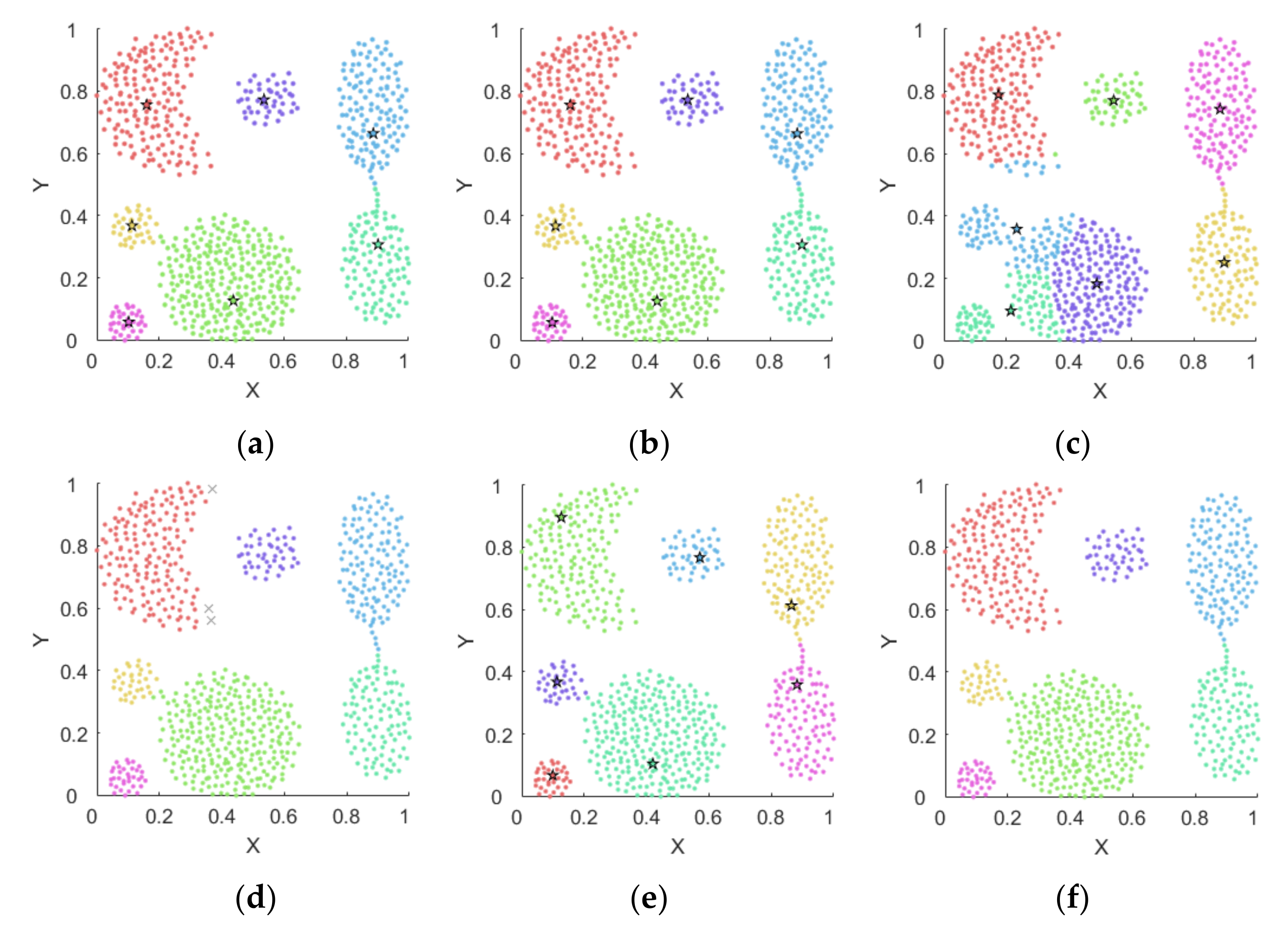
The Aggregation dataset has seven clusters. There is little difference in density among the seven clusters. The clustering effect of DPC algorithm on Aggregation is good. The similar density and uniform data distribution make the DPC algorithm applicable to this dataset. ConDPC also achieves a good clustering effect on Aggregation. The clustering result of K-means algorithm is poor. DBSCAN misjudges some points as noise points, and the clustering effect is mediocre. The clustering results are shown in Figure 3, and the star shaped points are the cluster centers [34].
The Flame dataset has two clusters. The shape of the two clusters is different and the density distribution is uniform. As can be seen from Figure 4, ConDPC, DPC, and McDPC have the best clustering effects.
R15 has a total of 15 clusters, as shown in Figure 5. These 15 clusters have similar densities and similar distributions. The DPC algorithm has achieved a good clustering effect on this dataset. The other five algorithms also have good clustering results.
The clustering effect on the latter two datasets is described below. DPC does not perform well on this kind of data set. This group of experiments mainly verifies the good clustering effect of ConDPC on these datasets.
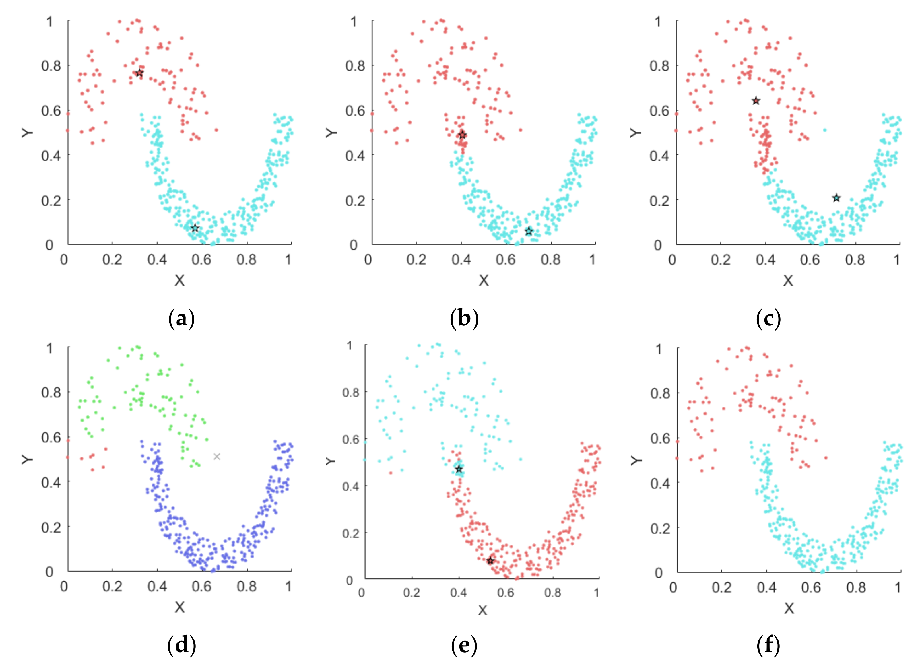
The Jain dataset consists of two lunar data clusters. The density of these two clusters is quite different, so Jain is often used to check the accuracy of the clustering algorithms. The density calculation of DPC does not consider the density difference between different clusters. In the Jain dataset, the density of the bottom cluster is significantly higher than that of the upper cluster. As shown in Figure 6b, DPC finds two center points in the bottom cluster.
After ConDPC finds the point with the highest density in a connected group, it will update δ value of this point to the maximum value. In this way, the corresponding γ is corrected. As a result, although the density of the upper cluster is sparse, for the point with the largest density in the cluster, its δ value is the maximum value, so its γ value increases accordingly, and finally, this point is selected as the clustering center. In this way, ConDPC finds the cluster centers in both clusters and correctly assigns the remaining points to the corresponding clusters. DBSCAN fails to distinguish multiple clusters with large density differences, divides the upper cluster into two, and misjudges a point as a noise point. Only DPC and McDPC implement clustering perfectly, as shown in Figure 6.
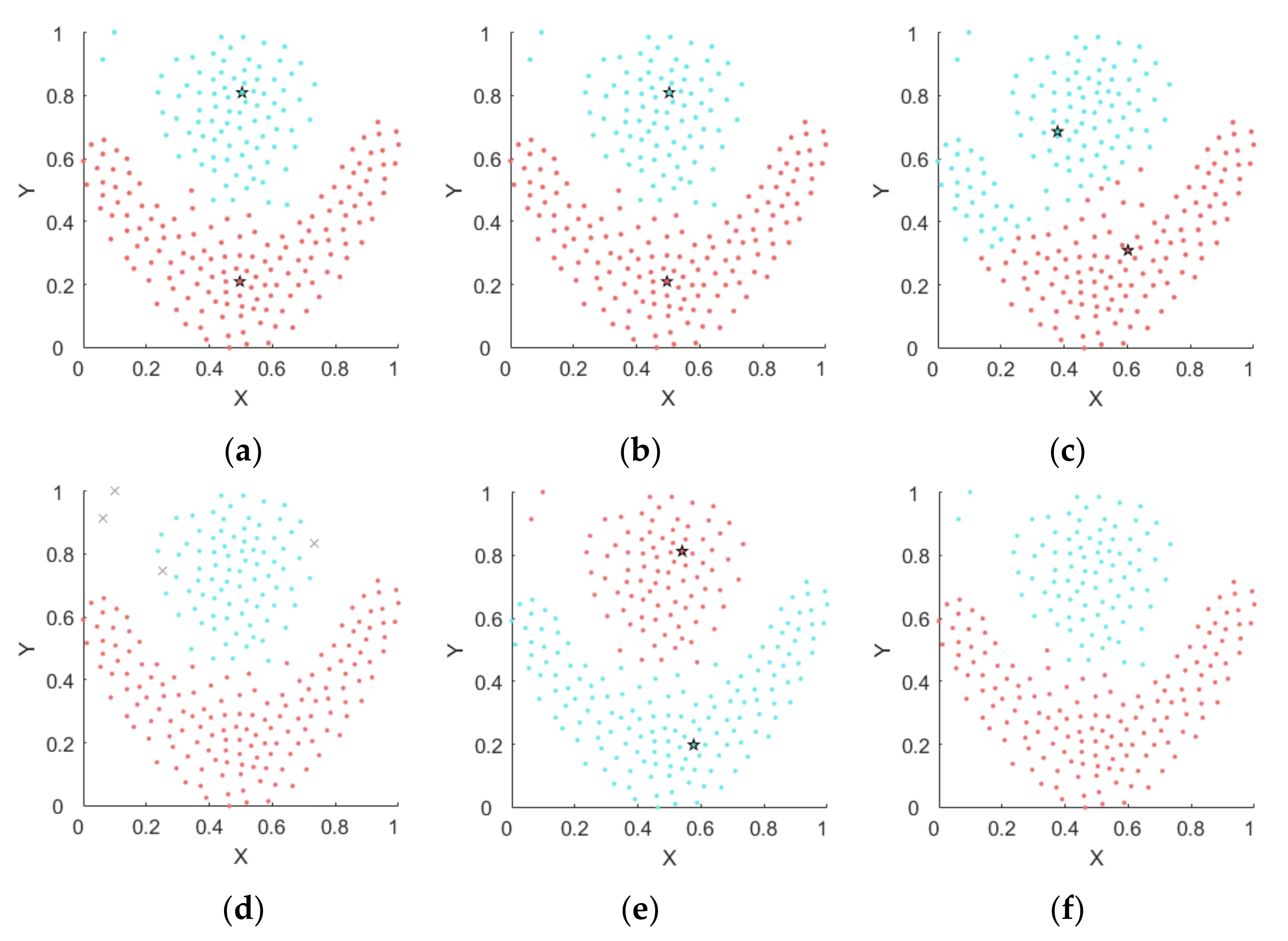
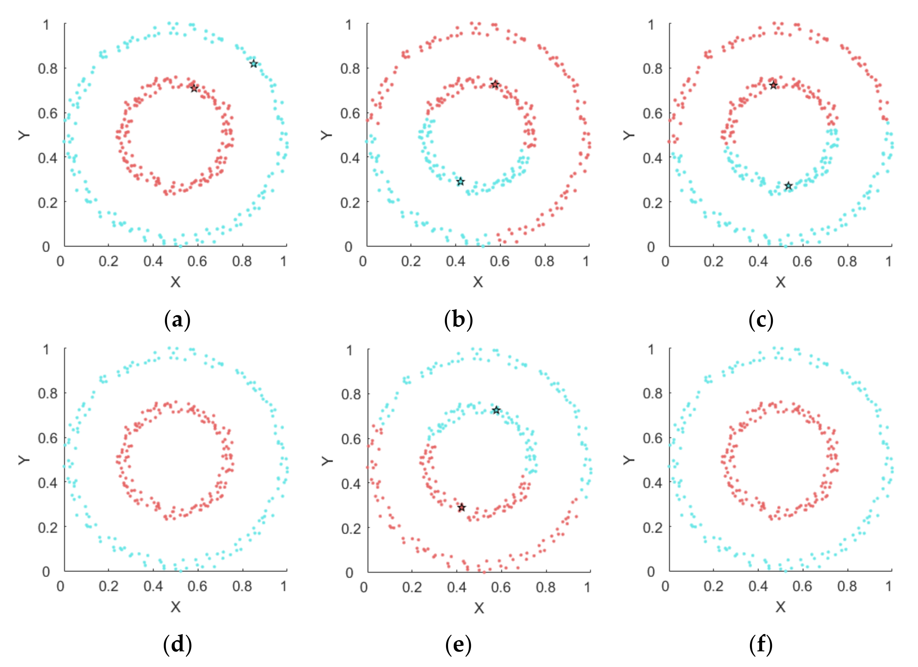
The Twocircle dataset consists of two nested circular clusters. The density of the internal circle cluster is higher than that of the external one. DPC does not consider the difference of different cluster densities and selects two points that are farther apart in the internal circle cluster with a higher density as the cluster centers but does not select the cluster center in the external circle cluster.
For the ConDPC algorithm, although the density of the external circle cluster is relatively small, for the point with the largest density in the cluster, its δ value is updated to the maximum value, so its γ value increases accordingly, and finally, this point is selected as the clustering center.
As can be seen from Figure 7, the clustering results of ConDPC, DBSCAN, and McDPC are perfect. However, DPC, K-means, and DPC-DBFN have poor clustering results on the dataset.
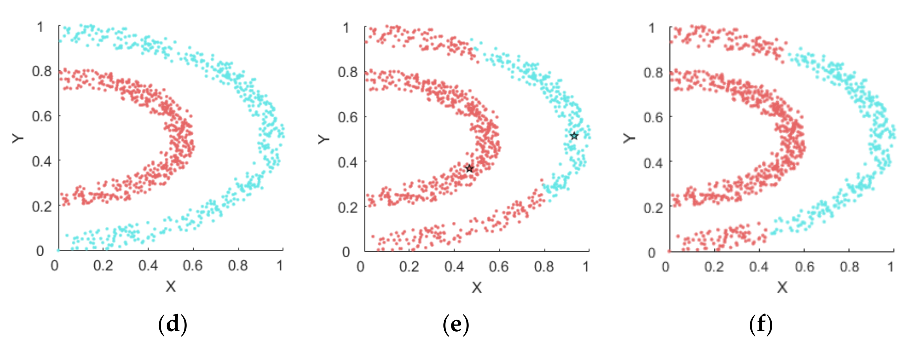
The Halfkernal dataset consists of two surrounding moon-shaped data clusters. The density of the two clusters is similar. When the DPC algorithm selects neighbors, it only considers the Euclidean distance between two points and does not consider the connectivity between the two points. As shown in Figure 2, DPC can find the clustering centers in the two clusters, respectively. However, in the process of neighbor selection, point p of the external cluster chooses point q of the internal cluster as its neighbor, resulting in many points of the external cluster being incorrectly assigned to the internal cluster.
ConDPC preferentially searches for big neighbors in the connected group where the point resides. Therefore, even if there are big neighbors closer to p in the internal cluster, they are not considered because they are not in the same connected group as p .
As shown in Figure 8, ConDPC selects the cluster centers in the two clusters, respectively, and assigns the remaining points to the corresponding clusters. DBSCAN also achieves a good clustering result. The other algorithms have poor clustering effects.
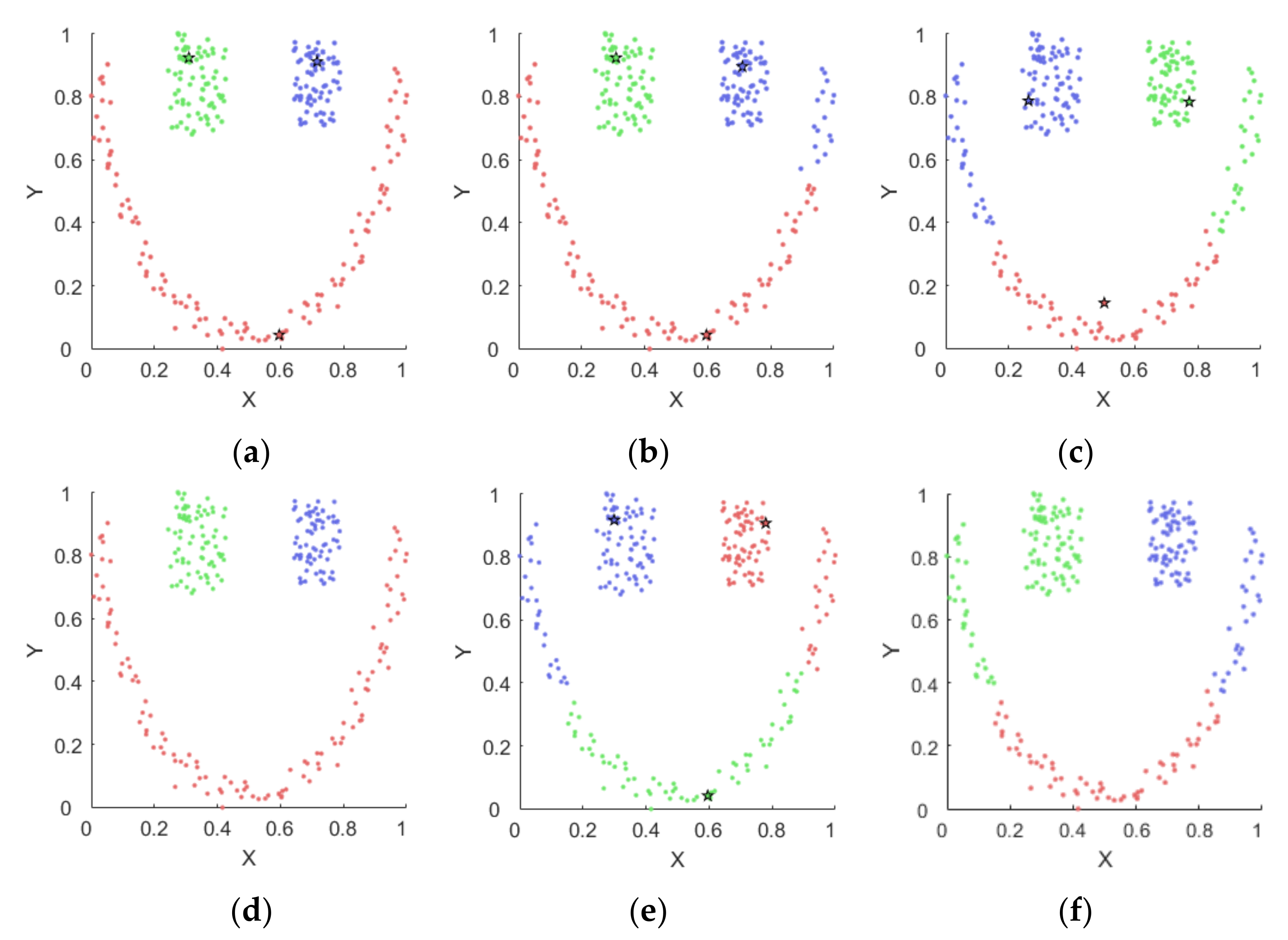
The Halfcirlce dataset consists of one moon-shaped cluster and two rectangle-shaped clusters, which is similar to the semi-enclosed structure as a whole. The three clusters have similar densities. As can be seen from Figure 9, DPC can find the appropriate clustering centers in each cluster. However, when assigning the points to the clusters, some points of the moon-shaped cluster are wrongly assigned to the rectangle-shaped cluster on the right. This is still because the original algorithm directly selects the nearest big neighbor to a given point without considering the connectivity between the two points when searching for the neighbor.
ConDPC preferentially searches for big neighbors in the connected group where the point resides. Therefore, even if there are big neighbors in the rectangle-shaped cluster that are closer to a point in the moon-shaped cluster, they are not considered because they are not in the same connected group as the point.
As shown in Figure 9, ConDPC selects the cluster center points in the three clusters, respectively, and assigns the remaining points to the corresponding clusters. DBSCAN also achieves a good clustering result. K-means and the last two improved algorithms produce similar poor results.
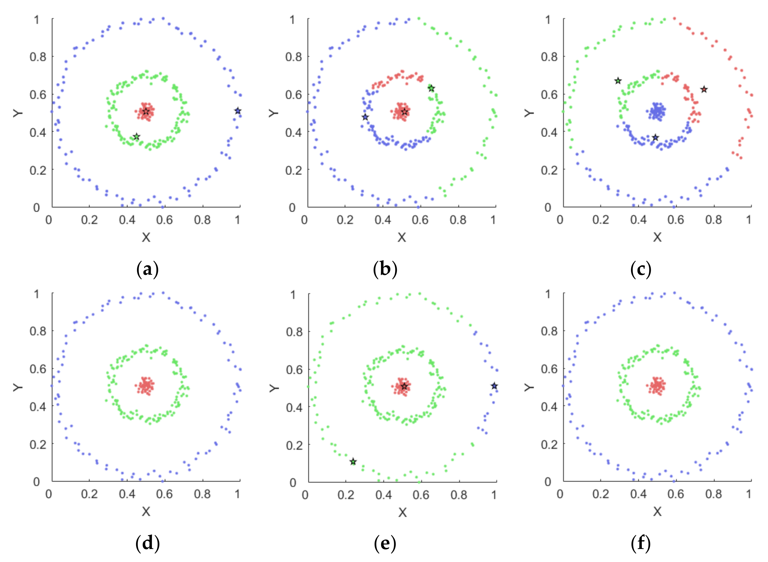
The Threecircle dataset is made up of three nested circles. The inner circle is denser than the outer circle. It can be seen from Figure 10 that: (1) DPC algorithm fails to correctly select the clustering center; (2) DPC algorithm fails to correctly assign the remaining points to the cluster. The DPC algorithm selects one cluster center in the inner circle with the largest density, two cluster centers in the middle circle, and no cluster center in the outer circle with the sparsest density. When the other points are assigned to the clusters, some points in the middle circular cluster are incorrectly assigned to the inner circular cluster.
ConDPC can find the appropriate cluster center in each cluster because it modifies the calculation method of neighbor distance. In addition, ConDPC preferentially searches for big neighbors in the same connected group, so the neighbors are searched correctly and assigned to the corresponding cluster.
As can be seen from Figure 10, the clustering results of ConDPC, DBSCAN, and McDPC are perfect. Both DPC and K-means get bad clustering results.
Table 3 shows the clustering comparison results on the synthetic datasets. From Table 3, we can see that the traditional DPC algorithm achieves good clustering results on datasets Aggregation, Flame, and R15. On the Jain and Twocircle datasets with obvious density differences, DPC finds multiple cluster centers in the dense cluster, but fails to find cluster centers in the sparse cluster, so the clustering effect is poor. DPC can find the clustering center point on the semi-enclosed datasets Halfkernal and HalfCircle. However, when assigning neighbors to other points, the points will be assigned to the wrong neighbor because the relative location structure of the data set is not considered, which leads to the wrong cluster allocation.
The proposed algorithm ConDPC has achieved good clustering results on the first three datasets. At the same time, on datasets with obvious density differences, ConDPC can find the corresponding center points in different clusters. On the datasets with enclosed/semi-enclosed distributions, ConDPC takes into account the data connectivity and preferentially searches for neighbors in the same connected group so that points can be correctly assigned to the corresponding clusters.
The visualization results from Figure 3, Figure 4, Figure 5, Figure 6, Figure 7, Figure 8, Figure 9 and Figure 10 and the index values in Table 3 show that the ConDPC algorithm has the highest accuracy among all comparison algorithms on the datasets.

4.2. Experiments on Real-World Datasets

4.2.1. Real-World Datasets

To verify the feasibility of the proposed algorithm, we also use real-world datasets for validation. The real datasets used in this experiment are from UCI Machine Learning Repository [35]. The detailed information of the data sets is shown in Table 4.

4.2.2. Results on Real-World Datasets

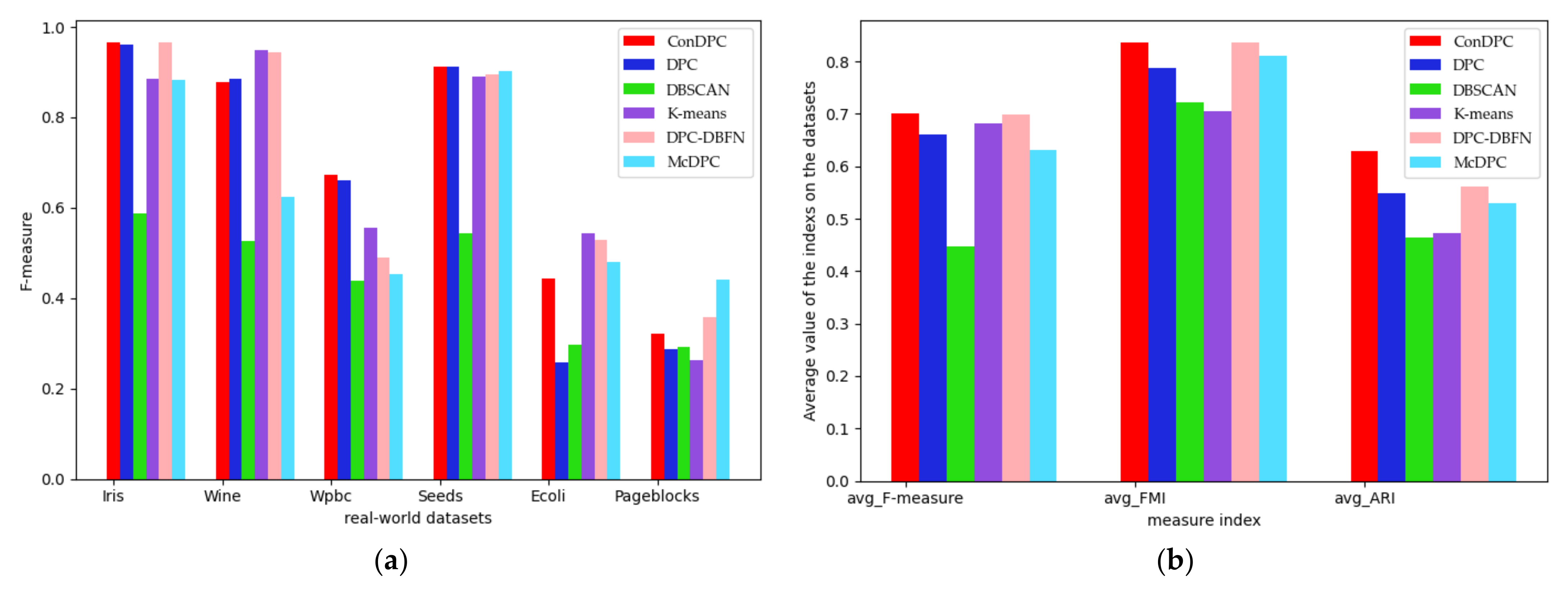
Table 5 shows the best clustering index values of the four algorithms on the six datasets. The last column is the average value of the clustering index of each algorithm on the datasets. Figure 11a shows the best F-measure result of each algorithm on each dataset, and Figure 11b shows the average index values of the algorithms on the six datasets.
It can be seen from Table 5 and Figure 11 that the average values of the three indexes corresponding to the ConDPC algorithm are the highest.

4.3. Experimental Discussion

ConDPC follows the input parameter settings of the original DPC. In the actual experiments, we set the range and step size of the input parameters of the two algorithms to be the same. We set the range of the input parameter p e r c e n t to [0.1, 9] and the step size to 0.1, and select the best result from the corresponding results.
In the experiments of artificial datasets in Section 4.1, the value of each clustering index of the DPC algorithm is the highest or equal to the highest. DPC has achieved good clustering results on the Aggregation, Flame, and R15 datasets. The parameter settings of ConDPC on these datasets are completely the same as those of DPC. In fact, the clustering centers, neighbor assignment, and final results obtained by ConDPC are also the same as those of DPC. ConDPC retains the advantage of good clustering effects of DPC on such datasets. DPC performs poorly on the other five datasets while ConDPC still achieves good clustering results.
In the experiments of real-world datasets in Section 4.2, it can be seen from the clustering index results that ConDPC obtains better clustering results than DPC does on most datasets. The average values of the three indexes of DPC are the highest, corresponding to the best comprehensive evaluation of the clustering results.

5. Conclusions

In this study, we proposed an improved density peak clustering algorithm ConDPC based on data connectivity. In this algorithm, the judgment of data connectivity is added to the original algorithm, and then the calculation of neighbor distance and the neighbor allocation rule are modified.
Experiments showed that ConDPC improves the accuracy of the original algorithm and expands the application scenarios. When the density of different clusters is different or the data distribution is nested, ConDPC can still achieve a good clustering effect.
The algorithm improves the accuracy of clustering, but it also takes a certain amount of time. The subsequent work will further consider the improvement of algorithm performance and apply the algorithm to specific businesses, such as AIS trajectory clustering.

Author Contributions

Conceptualization and methodology, Y.Z. and Z.W.; software, validation, visualization, investigation, resources, data curation, writing—original draft preparation, Y.Z.; writing—review and editing, Y.Z.; funding acquisition, Y.Z. All authors have read and agreed to the published version of the manuscript.

Funding

This research was funded by China Postdoctoral Science Foundation (No. 2019M651844), the Natural Science Foundation of the Jiangsu Higher Education Institutions of China (No. 21KJB580007), and the funding of the innovation science and technology project of Jiangsu Maritime Institute (No. 016102).

Institutional Review Board Statement

Not applicable.

Informed Consent Statement

Not applicable.

Data Availability Statement

The datasets underlying this article are cited and mentioned in the article.

Acknowledgments

We thank Juan Zhang, Jie Zhu and Taizhi Lv for their reviewing and editing of the manuscript and their funding acquisition work.

Conflicts of Interest

The authors declare no conflict of interest.

References

  1. Jain, A.K. Data clustering: 50 years beyond K-means. Pattern Recognit. Lett. 2010, 31, 651–666. [Google Scholar] [CrossRef]
  2. Han, J.; Kamber, M.; Pei, J. Data Mining: Concepts and Techniques, 3rd ed.; Morgan Kaufmann: Waltham, MA, USA, 2011; pp. 443–450. [Google Scholar]
  3. Zhu, Y.; Ting, K.M.; Carman, M.J. Density-ratio based clustering for discovering clusters with varying densities. Pattern Recognit. 2016, 60, 983–997. [Google Scholar] [CrossRef]
  4. Pavithra, L.K.; Sree, S.T. An improved seed point selection-based unsupervised color clustering for content-based image retrieval application. Comp. J. 2019, 63, 337–350. [Google Scholar] [CrossRef]
  5. Sun, Z.; Qi, M.; Lian, J.; Jia, W.; Zou, W.; He, Y.; Liu, H.; Zheng, Y. Image Segmentation by Searching for Image Feature Density Peaks. Appl. Sci. 2018, 8, 969. [Google Scholar] [CrossRef] [Green Version]
  6. Akila, I.S.; Venkatesan, R. A Fuzzy Based Energy-aware Clustering Architecture for Cooperative Communication in WSN. Comp. J. 2016, 59, 1551–1562. [Google Scholar] [CrossRef]
  7. Xu, Z.; Wang, M.; Li, Q.; Qian, L. Fault Diagnosis Method Based on Time Series in Autonomous Unmanned System. Appl. Sci. 2022, 12, 7366. [Google Scholar] [CrossRef]
  8. Ester, M.; Kriegel, H.P.; Sander, J.; Xu, X. A density-based algorithm for discovering clusters in large spatial databases with noise. In Proceedings of the KDD 96, Portland, OR, USA, 2–4 August 1996; pp. 226–231. [Google Scholar]
  9. Ankerst, M.; Breunig, M.M.; Kriegel, H.P.; Sander, J. OPTICS: Ordering points to identify the clustering structure. In Proceedings of the ACM SIGMOD International Conference on Management of Data, Philadelphia, PA, USA, 1–3 June 1999; pp. 49–60. [Google Scholar]
  10. Hinneburg, A.; Gabriel, H.H. Denclue 2.0: Fast clustering based on kernel density estimation. In Proceedings of the 7th International Symposium on Intelligent Data Analysis, Ljubljana, Slovenia, 6–8 September 2007; pp. 70–80. [Google Scholar]
  11. Sander, J.; Ester, M.; Kriegel, H.P.; Xu, X. Density-based clustering in spatial databases: The algorithm GDBSCAN and its applications. Data Min. Knowl. Disc. 1998, 2, 169–194. [Google Scholar] [CrossRef]
  12. Madhulatha, T.S. An overview on clustering methods. IOSR J. Eng. 2012, 2, 719–725. [Google Scholar] [CrossRef]
  13. Rodriguez, A.; Laio, A. Clustering by fast search and find of density peaks. Science 2014, 344, 1492–1496. [Google Scholar] [CrossRef] [Green Version]
  14. Du, M.; Ding, S.; Jia, H. Study on density peaks clustering based on k-nearest neighbors and principal component analysis. Knowl. Based Syst. 2016, 99, 135–145. [Google Scholar] [CrossRef]
  15. Xie, J.; Gao, H.; Xie, W.; Liu, X.; Grant, P.W. Robust clustering by detecting density peaks and assigning points based on fuzzy weighted K-nearest neighbors. Inf. Sci. 2016, 354, 19–40. [Google Scholar] [CrossRef]
  16. Lotfi, A.; Moradi, P.; Beigy, H. Density peaks clustering based on density backbone and fuzzy neighborhood. Pattern Recognit. 2020, 107, 107449. [Google Scholar] [CrossRef]
  17. Du, M.; Ding, S.; Xue, Y.; Shi, Z. A novel density peaks clustering with sensitivity of local density and density-adaptive metric. Knowl. Inf. Syst. 2018, 59, 285–309. [Google Scholar] [CrossRef]
  18. Wang, Y.; Wang, D.; Zhang, X.; Pang, W.; Miao, C.; Tan, A.; Zhou, Y. McDPC: Multi-center density peak clustering. Neural Comput. Appl. 2020, 32, 13465–13478. [Google Scholar] [CrossRef]
  19. Liu, Y.; Ma, Z.; Yu, F. Adaptive density peak clustering based on K-nearest neighbors with aggregating strategy. Knowl. Based Syst. 2017, 133, 208–220. [Google Scholar]
  20. Tao, X.; Guo, W.; Ren, C.; Li, Q.; He, Q.; Liu, R.; Zou, J. Density peak clustering using global and local consistency adjustable manifold distance. Inf. Sci. 2021, 577, 769–804. [Google Scholar] [CrossRef]
  21. Supplementary Materials for Clustering by Fast Search and Find of Density Peaks. Available online: https://www.science.org/doi/suppl/10.1126/science.1242072 (accessed on 20 September 2022).
  22. MacQueen, J.B. Some methods for classification and analysis of multivariate observations. In Proceedings of the 5th Berkeley Symposium on Mathematical Statistics and Probability, Berkeley, CA, USA, 21 June–18 July 1965 and 27 December 1965–7 January1966; pp. 281–297. [Google Scholar]
  23. Rijsbergen, V. Foundation of Evaluation. J. Doc. 1974, 30, 365–373. [Google Scholar] [CrossRef]
  24. Fowlkes, E.B.; Mallows, C.L. A method for comparing two hierarchical clusterings. J. Am. Stat. Assoc. 1983, 78, 553–569. [Google Scholar] [CrossRef]
  25. Vinh, N.X.; Epps, J.; Bailey, J. Information theoretic measures for clusterings comparison: Variants, properties, normalization and correction for chance. J. Mach. Learn. Res. 2010, 11, 2837–2854. [Google Scholar]
  26. Guan, J.; Li, S.; He, X.; Zhu, J.; Chen, J. Fast hierarchical clustering of local density peaks via an association degree transfer method. Neurocomputing 2021, 455, 401–418. [Google Scholar] [CrossRef]
  27. Zhou, W.; Wang, L.; Han, X.; Li, M. A novel deviation density peaks clustering algorithm and its applications of medical image segmentation. IET Image Process. 2022, 16, 3790–3804. [Google Scholar] [CrossRef]
  28. Gionis, A.; Mannila, H.; Tsaparas, P. Clustering aggregation. In Proceedings of the 21st International Conference on Data Engineering, Tokyo, Japan, 5–8 April 2005; pp. 341–352. [Google Scholar]
  29. Fu, L.; Medico, E. Flame, a novel fuzzy clustering method for the analysis of DNA microarray data. BMC Bioinf. 2007, 8, 3. [Google Scholar] [CrossRef] [PubMed]
  30. Veenman, C.J.; Reinders, M.J.T.; Backer, E. A maximum variance cluster algorithm. IEEE Trans. Pattern Anal. Mach. Intell. 2002, 24, 1273–1280. [Google Scholar] [CrossRef] [Green Version]
  31. Jain, A.K.; Law, M.H.C. Data clustering: A user’s dilemma. In Proceedings of the Pattern Recognition and Machine Intelligence, Kolkata, India, 20–22 December 2005; pp. 1–10. [Google Scholar]
  32. Ng, A.Y.; Jordan, M.I.; Weiss, Y. On spectral clustering: Analysis and an algorithm. In Proceedings of the 14th International Conference on Neural Information Processing Systems: Natural and Synthetic, Vancouver, BC, Canada, 3–8 December 2001; pp. 849–856. [Google Scholar]
  33. Zelnik-Manor, L.; Perona, P. Self-tuning spectral clustering. In Proceedings of the 17th International Conference on Neural Information Processing Systems, Vancouver, BC, Canada, 1 December 2004; pp. 1601–1608. [Google Scholar]
  34. Liu, R.; Wang, H.; Yu, X. Shared-nearest-neighbor-based clustering by fast search and find of density peaks. Inf. Sci. 2018, 450, 200–226. [Google Scholar] [CrossRef]
  35. UCI Machine Learning Repository. Available online: http://archive.ics.uci.edu/ml (accessed on 20 September 2022).
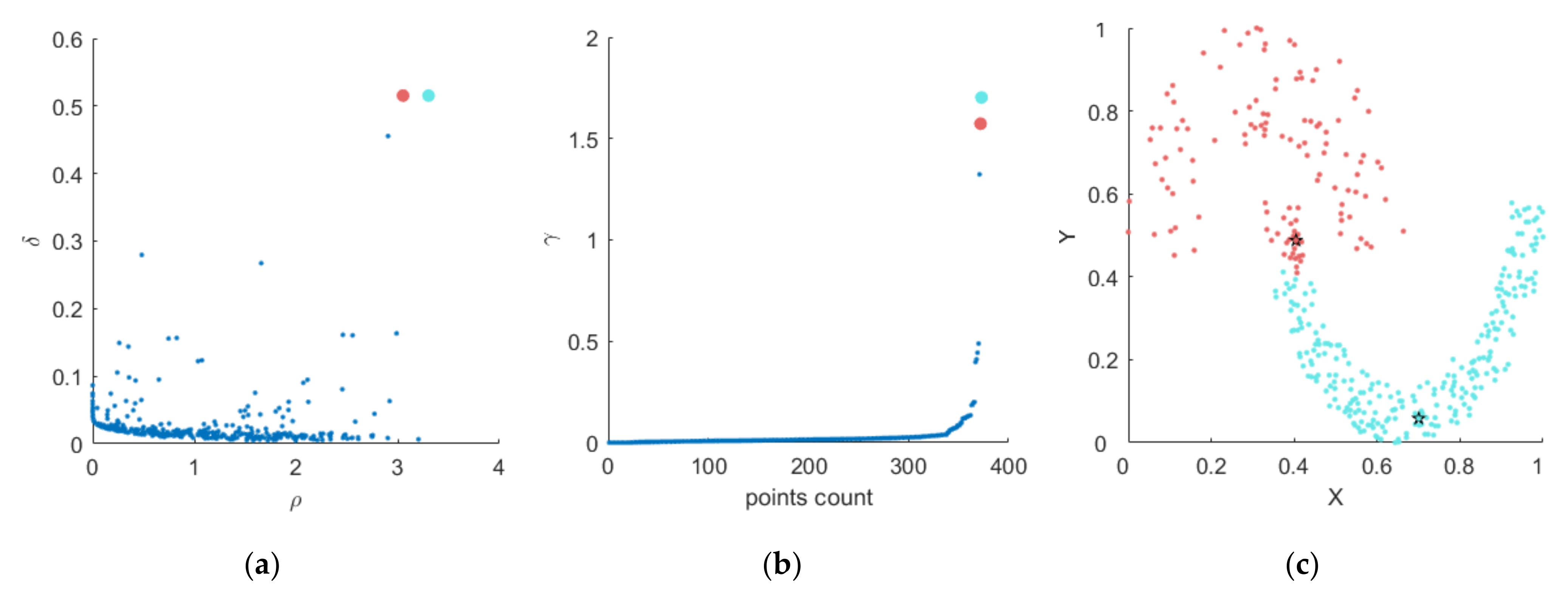
Figure 1. Best clustering result of DPC on Jain (percent = 0.3) (a) decision graph with ρ as x-axis and δ as y-axis; (b) distribution of γ value with points count as x-axis and γ as y-axis; (c) clustering result.
Applsci 12 12812 g001
Figure 2. Best clustering result of DPC on Halfkernal (percent = 5.6) (a) point p and its big neighbors; (b) point p and its neighbor point q ; (c) clustering result.
Applsci 12 12812 g002
Figure 3. Results on Aggregation. (a) ConDPC, (b) DPC, (c) K-means, (d) DBSCAN, (e) DPC-DBFN, (f) McDPC.
Applsci 12 12812 g003
Figure 4. Results on Flame. (a) ConDPC, (b) DPC, (c) K-means, (d) DBSCAN, (e) DPC-DBFN, (f) McDPC.
Applsci 12 12812 g004
Figure 5. Results on R15. (a) ConDPC, (b) DPC, (c) K-means, (d) DBSCAN, (e) DPC-DBFN, (f) McDPC.
Applsci 12 12812 g005
Figure 6. Results on Jain. (a) ConDPC, (b) DPC, (c) K-means, (d) DBSCAN, (e) DPC-DBFN, (f) McDPC.
Applsci 12 12812 g006
Figure 7. Results on Twocircle. (a) ConDPC, (b) DPC, (c) K-means, (d) DBSCAN, (e) DPC-DBFN, (f) McDPC.
Applsci 12 12812 g007
Figure 8. Results on HalfKernal. (a) ConDPC, (b) DPC, (c) K-means, (d) DBSCAN, (e) DPC-DBFN, (f) McDPC.
Applsci 12 12812 g008aApplsci 12 12812 g008b
Figure 9. Results on HalfCircle. (a) ConDPC, (b) DPC, (c) K-means, (d) DBSCAN, (e) DPC-DBFN, (f) McDPC.
Applsci 12 12812 g009
Figure 10. Results on ThreeCircle. (a) ConDPC, (b) DPC, (c) K-means, (d) DBSCAN, (e) DPC-DBFN, (f) McDPC.
Applsci 12 12812 g010
Figure 11. (a) F-measure of each algorithm on each dataset; (b) The average index values of each algorithm on the six datasets.
Applsci 12 12812 g011
Table 1. Information of the input parameters.
AlgorithmParameter(s) and the Search Range
ConDPC p e r c e n t { 0.1 , 0.2 , , 10 }
DPC p e r c e n t { 0.1 , 0.2 , , 10 }
DBSCAN e p s { 0.01 , 0.02 , , 0.09 } , M i n P t s { 2 , 3 , , 40 }
K-means n : number of clusters
DPC-DBFN k { 3 , 4 , , 40 }
McDPC γ { 0.01 , 0.02 , , 0.50 } , θ { 0.01 , 0.02 , , 0.50 } λ { 0.01 , 0.02 , , 1.00 } , p c t { 0.3 , 0.4 , , 6.0 }
Table 2. Information on the synthetic datasets.
DatasetSourceInstancesFeaturesClusters
Aggregation[28]78827
Flame[29]24022
R15[30]600215
Jain[31]37322
Twocircle[32]31422
Halfkernal[17]100022
Halfcircle[33]23823
Threecircle[33]29923
Table 3. Performances on synthetic datasets.
Algorithm AggregationFlameR15JainTwocircleHalfkernalHalfcircleThreecircle
ConDPCF-measure0.99810.99711111
FMI0.99710.99311111
ARI0.99610.99311111
Parameter3.12.73.432.71.53.87.2
DPCF-measure0.99810.9970.9100.6100.8190.9430.586
FMI0.99710.9930.8820.5340.7290.8840.492
ARI0.99610.9930.7150.0500.4220.8240.214
Parameter3.12.73.40.30.20.14.20.2
DBSCANF-measure0.9960.9790.9940.9761111
FMI0.9940.9740.9880.9901111
ARI0.9920.9440.9870.9761111
Parameter0.08/210.1/100.05/300.08/20.07/40.08/50.08/50.09/5
K-MeansF-measure0.8340.8330.9970.8640.5100.5220.7980.451
FMI0.7880.7360.9930.8200.4970.5060.6650.403
ARI0.7300.4530.9930.577−0.0030.0020.4880.053
Parameter721522233
DPC-DBFNF-measure0.9950.9910.9980.9250.5030.7430.8180.712
FMI0.9940.9850.9970.9060.4970.6740.6870.715
ARI0.9930.9670.9960.768−0.0030.2670.5220.476
Parameter306391447317
McDPCF-measure0.99810.997110.8190.7981
FMI0.99710.993110.7290.6651
ARI0.99610.993110.4220.4881
Parameter0.1/0.01/0.21/10.1/0.01/
0.4/5
0.05/0.01/
0.05/2
0.3/0.3/0.23/50.2/0.5/0.08/20.01/0.01/
0.21/5
0.3/0.5/0.3/20.3/0.5/0.08/2
Table 4. Information of the real-world datasets.
DatasetSourceInstancesFeaturesClusters
Iris[35]15043
Wine[35]178133
Wpbc[35]198322
Seeds[35]21077
Ecoli[35]33678
Pageblocks[35]5473105
Table 5. Performances on real-world datasets.
Algorithm IrisWineWpbcSeedsEcoliPageblocksAverage
ConDPCF-measure0.9670.8790.6730.9130.4440.3220.700
FMI0.9350.7750.7620.8440.7770.9260.837
ARI0.9040.6600.2440.7670.6920.4980.628
Parameter2.50.80.40.70.62.7
DPCF-measure0.9600.8850.6610.9130.2590.2870.661
FMI0.9230.7830.7600.8440.5060.9080.787
ARI0.8860.6720.2270.7670.3490.3870.548
Parameter0.22.07.40.70.48
DBSCANF-measure0.5870.5260.4390.5430.2980.2930.448
FMI0.7530.7180.5630.6940.7630.8480.723
ARI0.6250.538 0.0340.5240.6690.3920.464
Parameter0.13/90.51/230.64/40.3/350.23/300.08/33
K-MeansF-measure0.8850.9490.5550.8910.5430.2630.681
FMI0.8110.9030.5790.8030.5590.5830.706
ARI0.7160.8540.0320.7050.4250.1080.473
Parameter332385
DPC-DBFNF-measure
FMI
ARI
Parameter
0.967
0.935
0.904
5
0.945
0.888
0.832
3
0.489
0.721
0.004
19
0.896
0.809
0.715
4
0.530
0.755
0.658
3
0.358
0.914
0.254
39
0.698
0.837
0.561
McDPCF-measure
FMI
ARI
Parameter
0.883
0.816
0.720
0.1/0.1/0.34/1
0.625
0.680
0.439
0.2/0.3/0.6/1
0.452
0.787
0.008
0.2/0.52/0.3/0.3
0.903
0.826
0.742
0.02/0.02/0.3/0.3
0.480
0.822
0.739
0.02/0.01/0.3/0.5
0.440
0.928
0.524
0.01/0.01/
0.33/1
0.631
0.810
0.529
Publisher’s Note: MDPI stays neutral with regard to jurisdictional claims in published maps and institutional affiliations.