Article

Comparative Study of Lightweight Deep Semantic Segmentation Models for Concrete Damage Detection

1
Department of Civil Engineering, University of Seoul, 163 Seoulsiripdae-ro, Dongdaemun-gu, Seoul 02504, Republic of Korea
2
School of Civil, Architectural Engineering and Landscape Architecture, Sungkyunkwan University, 2066 Seoburo, Jangan-gu, Suwon 16419, Republic of Korea
3
Graduate School of Urban Bigdata Convergence, University of Seoul, 163 Seoulsiripdae-ro, Dongdaemun-gu, Seoul 02504, Republic of Korea
*
Author to whom correspondence should be addressed.
Appl. Sci. 2022, 12(24), 12786; https://doi.org/10.3390/app122412786
Submission received: 8 November 2022 / Revised: 6 December 2022 / Accepted: 8 December 2022 / Published: 13 December 2022
(This article belongs to the Special Issue Artificial Intelligence-Based Structural Health Monitoring)

Abstract

:
Innovative concrete structure maintenance now requires automated computer vision inspection. Modern edge computing devices (ECDs), such as smartphones, can serve as sensing and computational platforms and can be integrated with deep learning models to detect on-site damage. Due to the fact that ECDs have limited processing power, model sizes should be reduced to improve efficiency. This study compared and analyzed the performance of five semantic segmentation models that can be used for damage detection. These models are categorized as lightweight (ENet, CGNet, ESNet) and heavyweight (DDRNet-Slim23, DeepLabV3+ (ResNet-50)), based on the number of model parameters. All five models were trained and tested on the concrete structure dataset considering four types of damage: cracks, efflorescence, rebar exposure, and spalling. Overall, based on the performance evaluation and computational cost, CGNet outperformed the other models and was considered effective for the on-site damage detection application of ECDs.

1. Introduction

Structural health monitoring (SHM) is an essential way to prevent civil structures from damage as well as to improve their structural health via regular maintenance. SHM can be categorized into two approaches: vision-based inspection and sensor-based monitoring. The latter uses sensors installed on structures to continuously monitor structural changes by measuring structural responses, including displacement, strain, and acceleration. Vision-based inspection finds apparent damage or phenomena caused by structural damage, which have been recently observed, using optical devices combined with various computer vision (CV) techniques. The recent advances in CV techniques have had a high impact on today’s SHM of civil structures. These techniques are generally noncontact, remote, and quick, with minimal interference to structural operation; hence, such CV techniques are promising as a supplement to conventional labor-based inspection.
The inspection of concrete infrastructure is important, as these structures experience degradation through aging, earthquakes, or overloading. The degradation becomes apparent in the form of damage, such as cracks, spalling, rebar exposure, rebar corrosion, segregation, and efflorescence. Various studies have reported the detection of such damage using CV techniques [1,2,3]. Over the last decade, machine learning algorithms, such as k-means and self-organizing maps (SOMs), support vector machines (SVMs), naive Bayes classifiers, and feed-forward neural networks (FNNs), have been applied to detect various types of structural damage [4,5,6]. However, following the evolution of convolutional neural networks (CNNs) and an increase in the amount of data, deep learning architectures have been widely used for damage detection in concrete structures [7,8,9]. Cha et al. [10] conducted a comparative study on crack detection to compare the CNN-based approach with the traditional Canny and Sobel edge detection methods. Zhang et al. [11] proposed a crack-detection model using fully convolutional layers with different dilation rates for feature-map extraction. Kim and Cho [12] conducted a study on crack morphology detection using a CNN-based architecture known as AlexNet. Yang et al. [13] used three object detection models (AlexNet, VGGNet13 and ResNet18) for crack detection in concrete structures. Many studies have proposed crack detection and localization using deep learning models [14,15,16]. Ali et al. [17] proposed a customized CNN-based model approach for crack detection and localization, which outperformed other pre-trained object detection models in terms of accuracy.
To quantify the detected damage, damage must be both detected and pixel-wise segmented. Regarding pixel-wise segmentation, many researchers have used semantic and instance segmentation deep-learning models [18,19,20] for inspection. Hsieh and Tsai [21] conducted a review of pixel-level crack segmentation and compared eight different deep learning models with a performance evaluation. Kim et al. [22] used an artificial neural network for crack segmentation. They also proposed algorithms to analyze the length and width of cracks, known as thinning and tracking algorithms. Zhou and Song [23] proposed an encoder–decoder network called CrackNet for crack segmentation on a concrete roadway. In addition to concrete crack segmentation, Junior et al. [24] proposed a deep learning architecture for crack segmentation on ceramic tiles. The authors focused on cracks irrespective of the background, and detected and separated cracks close to the grout.
Damage, such as spalling, rebar exposure, and efflorescence, can occur in any concrete structure, along with cracks, and they are significant indicators of structural integrity. Efflorescence is a white salt residue that occurs mainly in areas with low temperatures and moist conditions. Spalling or potholes occur when water in a concrete structure undergoes multiple freeze–thaw cycles or when the rebar inside the concrete swells due to corrosion. Rebar exposure mainly occurs in concrete structures owing to the pouring of concrete mixtures with water deficiency or spalling. It is usually accompanied by spalling or cracks and is always detected with other concrete damage [25]. Li et al. [26] modified a fully convolutional network to detect multiple forms of damage via semantic segmentation in concrete structures, including cracks, spalling, rebar exposure, and holes. Shi et al. [27] detected corrosion and cracks by improving segmentation accuracy using two methods of data input: (i) squashing segmentation, to input images with high resolution and (ii) cropping segmentation, to crop the image into a desired resolution. Although deep learning model performances are material-specific, their performances were found to be inadequate when a pre-trained model was tested on different material images with the same task [28]. Therefore, Hoskere et al. [29] proposed a multi-task semantic segmentation model called MaDnet to detect multiple forms of damage in concrete, steel, and asphalt. For real-time damage detection, many studies have been conducted using fast R-CNN [30] and mask R-CNN [31]. Wang et al. [32] used the fast R-CNN model to detect multiple forms of damage in real-time masonry structures. Kim and Cho [33] proposed a study based on mask R-CNN for instance segmentation, and they detected multiple forms of damage in a concrete structure.
The abovementioned studies sought to achieve better damage detectability by implementing highly complex models with numerous trainable parameters. Thus, the models in these studies performed well on high-performance computers with several GPUs. However, in the past decade, various small edge computing devices (ECDs) have become available, including smartphones, Jetson, Coral, Raspberry Pi, and Arduino [34,35,36]. These ECDs connect to, or can be easily integrated with, imaging sensors, and they can be used by practitioners to build portable inspection devices that can detect and quantify damage to the field. In particular, smartphones have improved dramatically in terms of processors, memory, batteries, and communication; thus, smartphones have recently been used in various SHM applications [37,38,39]. To use ECDs as the operating platforms of deep learning models, lightweight models with a relatively small number of tunable parameters and appropriate performance are preferred. Howard et al. [40] proposed a lightweight network known as MobileNet for object classification. The authors introduced depth-wise separable convolution instead of standard convolution, resulting in a lightweight network, by decreasing the parameters from 29.3 million to 4.2 million. Cai et al. [41] proposed the YOLObile framework, which is a real-time object detection model for mobile devices. They implemented their model on a mobile device (Samsung Galaxy S20) and achieved an inference speed of approximately 17 FPS. In addition to classification and detection models, some research studies have been conducted on lightweight semantic segmentation models. Paszke et al. [42] proposed the first lightweight semantic segmentation model, known as ENet, which constitutes only 0.4 million parameters. Subsequently, other state-of-the-art models have been proposed that are supposed to be efficient for mobile devices [43,44,45]. However, the application of these models to damage segmentation tasks has rarely been reported in the literature.
In summary, the main contributions of the proposed study are as follows:
  • Three lightweight models (ENet) [42], context-guided network (CGNet) [45], and efficient symmetric network (ESNet) [46]) and two heavyweight models (deep dual-resolution network (DDRNet) [47] and DeepLabV3+ [48]) were compared for damage segmentation from structural images to investigate the best model that could be embedded in edge computing devices with less computational power.
  • A concrete dataset that contains four types of concrete damage, i.e., cracks, efflorescence, spalling, and rebar exposure, was constructed for training and testing of the semantic segmentation models. Images were collected from online and real concrete structures in South Korea.
  • The lightweight segmentation models were benchmarked for the detection of multiple types of concrete damage, and the tradeoff between the number of model parameters and accuracy was investigated.
After fair training of the models using the same training images, the inference performance on the test images was evaluated in terms of detectability and computation. Detectability was measured using mean intersection over union (mIoU) and F1-score, and the computation was measured using floating-point operations (FLOPs), as well as inference speed on a computer with GPUs.

2. Semantic Segmentation Models for Multi-Damage Detection

To study the tradeoff between the model parameters and accuracy, we chose five deep segmentation models to detect multiple types of damage in concrete: three lightweight models (ENet, CGNet, and ESNet) and two heavyweight models (DDR-Slim and DeepLabV3+). Brief descriptions of these models are provided below.

2.1. Efficient Neural Network (ENet)

Paszke et al. [42] proposed an efficient lightweight deep neural network (ENet) for semantic segmentation tasks. It is a state-of-the-art model with very low parameters (0.4 million) and FLOPs. The ENet was trained and tested on three types of datasets with different numbers of classes. For the Cityscapes dataset [49], with 19 classes, and the CamVid testing dataset [50], with 11 classes, the mIoUs of ENet were reported as 58.3% and 51.3%, respectively. Figure 1a shows the ENet initial block, containing the convolutional and max-pooling layers with concatenation. The initial block was first used in the encoder part to downsample the input image resolution to half. Figure 1b depicts the ENet bottleneck module, which consists of three convolutional layers, two max-pooling layers, and a regularizer. The 1 × 1 convolutional layer was used for the projection and expansion of the input features. The convolutional layer was dilated at different ratios to perform classification with a large receptive field. A spatial dropout [51] regularizer was placed at the end of the convolutional layers in the bottleneck module to avoid overfitting issues that could be caused by a small training dataset. The ENet architecture comprises five sections that contain the initial block and bottleneck modules. Several bottleneck modules were used in Section 1, Section 2 and Section 3 to further downsample the input image resolution to 1/8. Batch normalization (BN) and a parametric rectified linear unit (PReLU) were used after each convolutional layer to reduce the computational cost. The PReLU is an activation function that generalizes the conventional rectified unit by incorporating a negative slope. PReLU enhances model fitting with negligible additional computational expense and minimal overfitting risk [52]. The ENet architecture is different from other encoder–decoder models because the decoder module in ENet has fewer layers than the encoder. This was prompted by the idea that the encoder should be able to function on lower-resolution data and provide information processing and filtering in a manner similar to the original classification architectures. Section 4 and Section 5 describe the decoder part for the upsampling of the feature map, and very few bottleneck modules were used, compared with the encoder.

2.2. Context Guided Network (CGNet)

Wu et al. [42] proposed a context-guided network (CGNet) as a lightweight semantic segmentation model. CGNet contains only 0.5 million trainable parameters, which saves memory footprint and is considered suitable for implementation on ECDs. The performance of CGNet was evaluated using the Cityscapes and CamVid datasets, and it outperformed the other lightweight models, in terms of accuracy and computational cost. The architecture of the CGNet is simple and constitutes many CG blocks. Figure 2 presents the hierarchy of the CG block used for feature extraction. The CG block comprises two primary stages. In the first stage, floc(*) and fsur(*) are used to learn the local features and the relevant surrounding context. The floc(*) is a 3 × 3 depth-wise convolutional layer was employed for learning the local features from the eight adjacent feature vectors. Meanwhile, fsur(*) is a 3 × 3 depth-wise dilated/atrous convolutional layer for a large receptive field to efficiently learn the surrounding context. The depth-wise convolutional layer in both floc(*) and fsur(*) helped to significantly reduce the number of parameters in CGNet. Furthermore, fjoi(*) extracts joint features from the outputs of floc(*) and fsur(*). The fjoi(*) is simply designed as a concatenation layer, followed by the BN and PReLU operators. Stage two involves fglo(*), which consists of global average pooling, followed by two fully connected layers that extract the global context to improve the joint features. Joint features are refined channel-wise by applying the global context as a weighted vector to enhance relevant features and minimize irrelevant features.
Figure 3 represents the entire CGNet architecture. The encoder part comprises three stages for downsampling the input image resolution, as well as many CG blocks. In stage 1, the downsampling ratio is half, constituting three standard convolutional (3 × 3) layers, followed by the BN and PReLU operators. In stage 2, the input image passes through three CG blocks that downsample the resolution to 1/4. The dilation rate for fsur(*) in the CG blocks of stage 2 was 2. In stage 3, the input image is passed through 21 CG blocks and further downsampled to 1/8. The dilation rate for fsur(*) in the CG blocks of stage 3 was 4. Finally, the decoder part, to visualize the prediction of CGNet, employs an upsampling layer to resize the prediction into its original input resolution.

2.3. Efficient Symmetric Network (ESNet)

An efficient symmetric network (ESNet) is another lightweight state-of-the-art model that was proposed by Wang et al. [46]. ESNet consists of only 1.6 million parameters and is considered appropriate for embedding into ECDs. The ESNet was trained on the Cityscapes dataset, and its performance was compared with other lightweight models. ESNet achieved 70.7% mIoU on the Cityscapes testing dataset and achieved better performance, in terms of accuracy and inference speed, compared with other models in the study. To reduce the computational cost, ESNet employed two types of residual modules, known as factorized convolutional units (FCUs) and parallel FCUs (PFCUs), in their encoder and decoder parts. These are non-bottleneck modules, in which the standard convolution is decomposed into two 1D convolutional layers.
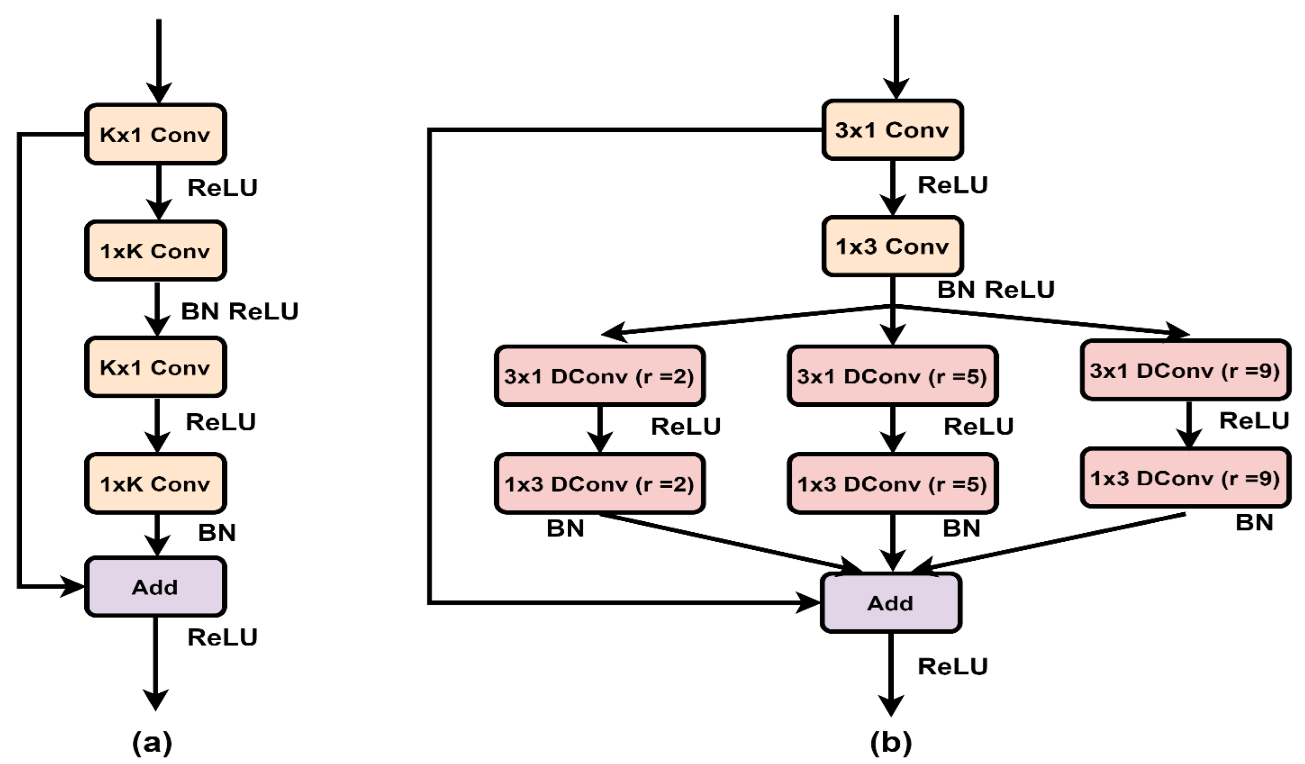
Figure 4a shows the entire FCU block, which consists of three decomposed 1D convolutional layers with addition, and each convolutional layer is followed by a rectified linear unit (ReLU) activation function with BN. K in Figure 4a represents the kernels size, which is not fixed to vary the receptive fields, depending on the feature map.
Figure 4b shows the PFCU block consists of decomposed 1D convolutional layers and adopts a transform–split–transform–merge strategy. The PFCU comprises two decomposed 1D convolutional layers that are then connected to three parallel dilated 1D convolutions. The dilation rates in the corresponding convolutional layers are 2, 3 and 5, and the outputs from these three dilated convolutions are added.
Figure 5 displays the entire architecture of ESNet, which is symmetric with the same number of layers in the encoder and decoder. The encoder part of the ESNet contains three blocks. Block 1 consists of three FCU modules, whose filter size (K) is 3, to downsample the input image to half. Block 2 consists of two FCU modules, with K of 5, to capture a wide-scaled context, and the downsampling ratio in this block is 1/4. Three PFCU blocks are used in block 3 to further downsample the input to 1/8 of its original resolution. For upsampling, the decoder comprises two blocks. Blocks 4 and 5 contain two FCU modules with filter sizes of 5 and 3, respectively. In blocks 4 and 5, the upsampling layer is employed in front of each FCU unit to resize the output to its original resolution map.

2.4. Deep Dual-Resolution Network (DDRNet-23-Slim)

Hong et al. [47] proposed a family of networks known as deep dual-resolution networks (DDRNet) for real-time road scene semantic segmentation. To investigate the tradeoff between accuracy and speed, they proposed different networks with several layers. DDRNet-23-Slim achieved better performance and inference speed, with a low reduction in accuracy. DDRNet-23-Slim contains approximately 5.7 million parameters and has been tested on both the Cityscapes and CamVid datasets. DDRNet-23-Slim achieved approximately 77.4% mIoU on the Cityscapes test dataset with the inference speed of 102 FPS, and 74.7% mIoU with the inference speed of 230 FPS on the CamVid test dataset. Figure 6 depicts the architecture of the DDR-Net, which comprises several modules known as sequential residual basic block, single residual bottleneck block, deep aggregation pyramid pooling module (DAPPM), and segmentation head (seg head). All modules contain different types of convolutional layers with varying filter sizes to downsample the input image resolution. First, the input image was downsampled to 1/64 of its resolution; subsequently, these low-resolution feature maps were connected to the DAPPM module. DAPPM contains large pooling kernels that further downsample the feature maps to 1/128, 1/256, and 1/512 of the input image resolution. After downsampling, both feature maps of resolutions 1/64 and 1/512 were concatenated and added to the seg head module, comprised of a, 3 × 3, standard convolutional layer, followed by a 1 × 1 convolution. Finally, the output from the seg head was upsampled to its original input resolution for segmentation prediction.

2.5. DeepLabV3+ (ResNet-50)

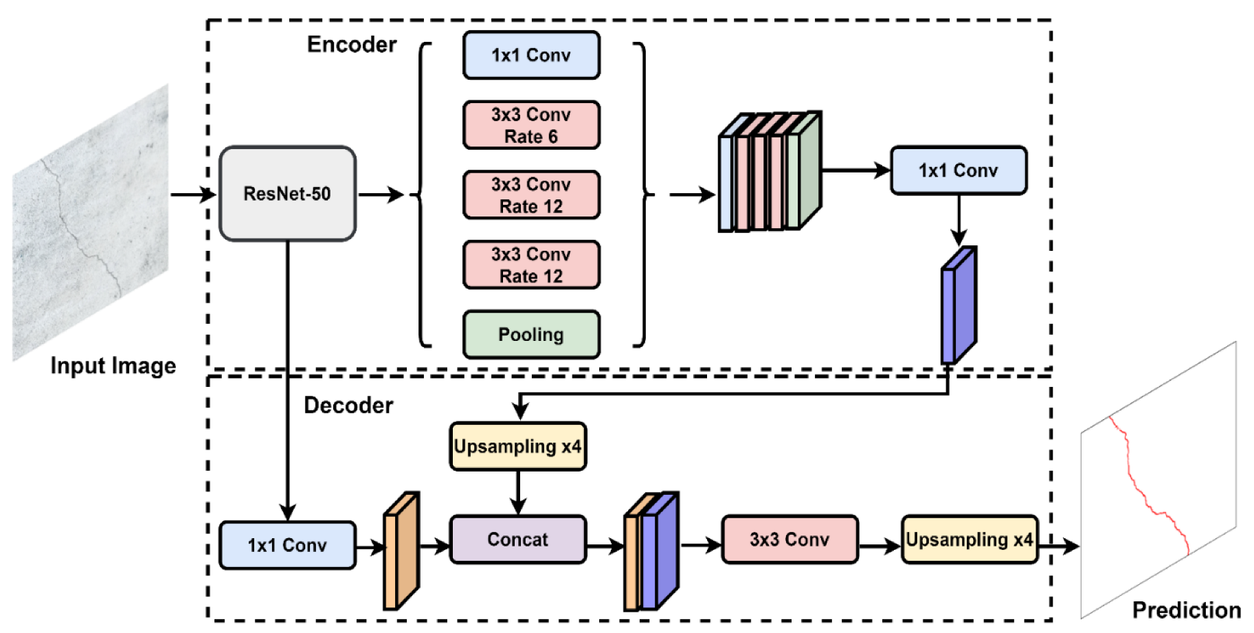
DeepLabV3+ is an encoder–decoder network and is a modified version of DeepLabV3 proposed by Chen et al. [48]. It contains numerous trainable parameters and is considered to be efficient for complex dataset segmentation. DeepLabV3+ was trained and tested on both the PASCAL VOC 2012 [53] and Cityscapes datasets, which achieved approximately 89% and 82.1% mIoU, respectively. In the encoder part shown in Figure 7, any deep CNN (DCNN) can be used as a backbone network for dense feature extraction. ResNet-50 was used as the backbone network in this study. The atrous spatial pyramid pooling (ASPP) module in the encoder uses multiple dilated convolutions at varying rates to improve feature extraction for high-level features. The ASPP probes an input convolutional feature layer with filters that have different sampling rates and effective fields of view. This allows it to capture both the objects and the context of an image at different scales. In the encoder part, the input was downsampled to 1/8 of the original resolution.
The decoder module is used to upsample the feature map obtained by the encoder into its original resolution. First, depth-wise separable convolution is applied to both high- and low-level features to reduce the computational cost and parameters. Subsequently, high-level features are upsampled by the ratio of four and concatenated with low-level features. To refine the features better, some 3 × 3 standard convolutions are applied after concatenation, and then the features are upsampled by the ratio of 4 to reconstruct the features into the corresponding input resolution.

2.6. Loss Functions for the Five Models

The loss function plays a vital role in the training of any deep-learning model. The loss function was used to calculate the prediction error of the model during training and to calculate the gradient to update the weights of the model accordingly. The loss function is typically determined by considering the task of the model, such as regression, binary classification, and multiclass classification. This study aimed to detect multiple types of damage in the images, so the categorical cross-entropy loss [54], expressed in Equation (1), was used to train all five models in this study:
L = i = 1 n j = 1 c y ij log   y ^ ij
Here, L denotes the cross-entropy loss, n is the number of pixels, c is the number of classes in the data, and y ij and   y ^ ij are the true labelled and predicted values of the i th example pixel corresponding to the j th class, respectively.

3. Details for Model Training and Evaluation

This section describes the dataset used for training and testing, the details of training, including hyperparameters, and the evaluation metrics used for the evaluation of detectability.

3.1. Concrete Dataset

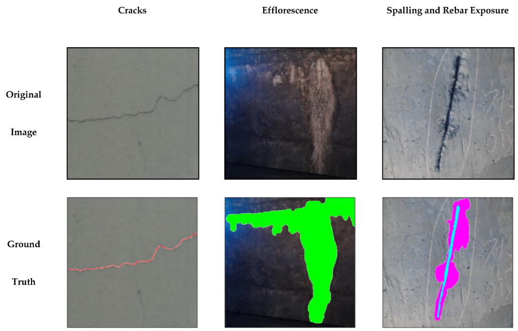
To evaluate the performance of the models, an image dataset containing concrete damage, was constructed. The images were collected from different sources, including online sources, as well as from real concrete structures in South Korea. Images in the dataset contained four types of damage: cracks, efflorescence, spalling, and rebar exposure. A total of 3840 images was used, of which 90% (3440 images) were used for training and 10% (400 images) for testing the models. The images had varying resolutions, starting from a high resolution of 1600 × 1200 to a lower resolution of 796 × 716 in RGB format. For pixel-level classification, the data was labelled manually using an Adobe Photoshop labelling tool to create the ground truths. Figure 8 shows an example of the four types of damage in the concrete dataset with the corresponding ground truths. The damages were labeled using different colors: cracks in red, efflorescence in green, spalling in magenta, and rebar exposure in cyan. The background was not labeled and is shown in white in the ground truth.

3.2. Training Details

Five models were trained on the Python IDE platform using the TensorFlow and Keras [55] libraries. Experiments were conducted on a workstation with two Intel Xeon processor CPUs and four NVIDIA RTX Titan GPUs with 64-GB RAM. The models were trained on multiple GPUs as distributed training, which helped increase the batch size and reduced the training time. During the training, 50% of the training data were randomly selected and augmented at every epoch. Two types of data augmentation options were used on the training images: (1) random flip right and left, and (2) random scale of 1–1.5. All models were trained from scratch, except DeeplabV3+(ResNet-50). To train the deep learning model from scratch all the learnable model parameters, like weights (convolution filters) were initialized randomly according to the input data during training and loss was calculated after each iteration. These model parameters were monitored by loss function and the training stopped when the loss minimized and was close to zero. Models like DeepLabV3+ used backbone network (ResNet-50) for classification tasks and decoder head for semantic segmentation. This backbone network used pretrained weights of ImageNet, excluding last fully connected layer, and helped the model to optimize quickly during training, also known as transfer learning. In this study DeepLabV3+ also used pretrained weights in the encoder module ResNet-50 as transfer learning. All models had an input image resolution of 680 × 680. The global batch size for training was 16 (four per GPU) and a total of 60 K iterations were set to train the models. An adaptive momentum (ADAM) [56] optimizer was employed to effectively train the model by adaptively changing the learning rate. The learning rate was scheduled, starting from 0.001 changes at each iteration and ending at 0.0001 at the completion of training.

3.3. Evaluation Metrics

To evaluate the detectability of trained segmentation models, two widely used metrics were introduced: (pixel-wise) F1 score and intersection over union (IoU). The F1 score is the harmonic mean of the precision and recall and is given by Equation (2):
F 1 - score = 2 Precision     Recall Precision + Recall
The precision and recall can be calculated using:
Precision = TPs TPs + FPs
Recall = TPs TPs + FNs
where true positives (TPs) are the overlapping pixels between the prediction and ground truth, false positives (FPs) are the non-overlapping pixels of the prediction, and false negatives (FNs) are the non-overlapping pixels of the ground truth. Precision assesses the model’s reliability in classifying positive samples, while recall assesses the model’s detectability on positive samples. By calculating the harmonic mean of the precision and recall, the F1 score provides a balanced measure of both reliability and detectability.
The IoU, also known as the Jaccard coefficient, is a commonly used metric for semantic segmentation tasks and can be described as the area of intersection of prediction with the ground truth, divided by the total area of the union of prediction and ground truth. The IoU can be expressed using TPs, FPs, and FNs, as shown in Equation (5):
IoU = TPs TPs + FPs + FNs

4. Results and Discussion

This section describes the experimental results of all the deep learning models used in this study. The models were compared in terms of their performance and computation. Note that all trained models were tested on 400 testing images of the concrete dataset.

4.1. Predicted Results Visualization

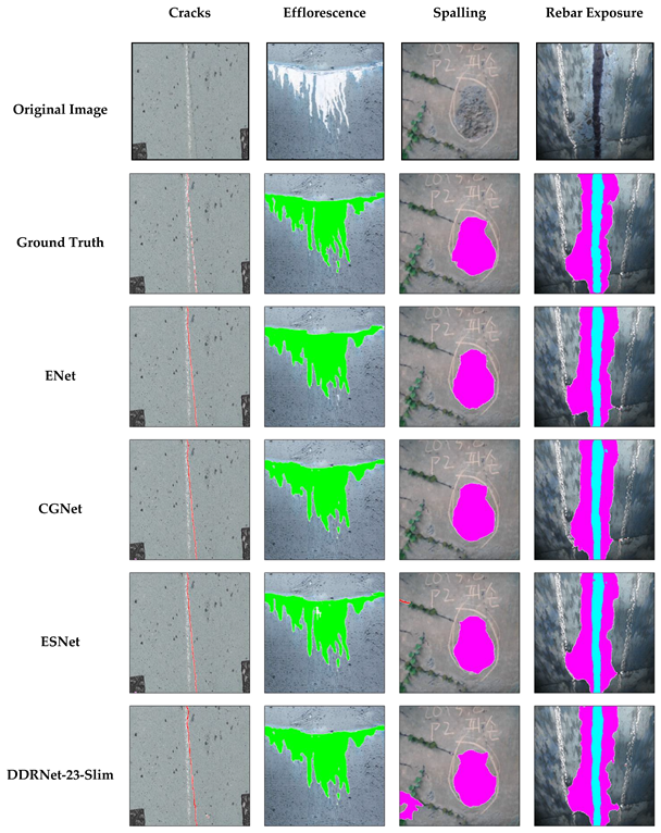
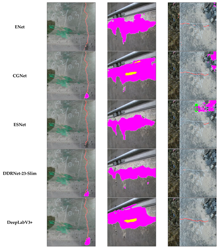
For the qualitative analysis of the segmentation performance of all the models, some prediction results for the test dataset are illustrated in Figure 9. The results are presented for each model corresponding to each damage class, with the raw image and pixel label ground truth from top to bottom. From the visual inspection, all models successfully predicted damage; however, some false alarms or FPs were observed in some prediction images. In the crack predictions, the models predicted the cracks but with a different pattern, compared to the ground truth. In the ground truth, the crack was labeled as non-continuous with a fine texture; however, the predictions were continuous and coarser than the ground truth. In the efflorescence class, it is evident from Table 1 that all models achieved better accuracy and an IoU of more than 50%. However, in the prediction, models predicted efflorescence with the same pattern as the ground truth, but some labels were missing and predicted as background, instead of efflorescence. The third column in Figure 9 shows the prediction results for the spalling class. In the background of the spalling image, there are parts of the climber or creeper plant. As a result, of this noisy and complex background, some false predictions were observed in the results of ESNet and DDRNet-23-Slim; however, overall, each model achieved better accuracy in the spalling class. The rebars in the concrete structure were mainly exposed after spalling; hence, the fourth column in Figure 9 displays the rebar exposure surrounded by spalling. All the models predicted rebar exposure with a minor pattern difference when compared with the ground truth.
Figure 10 illustrates some of the prediction results for all models with multiple classes and background noise. Noise in the background, or varied lighting conditions, in an image can significantly impact the performance of a deep learning model. For this purpose, the performance of each model was analyzed and compared. The first example includes the prediction of crack and spalling classes in parallel. Only CGNet predicted both types of damage in the lightweight models; however, certain spalling pixels were not predicted. DDR-23-Slim and DeepLabv3+, meanwhile, predicted spalling in the same manner as CGNet. In the case of spalling and rebar exposure, all models, except CGNet and DeepLabV3+, failed to detect rebar exposure. In the last example, in Figure 10, the image contained only cracks, and in the background, some stones were visible at the right corner of the image. In the prediction of all models, except DeepLabV3+, there were false alarms and missing crack labels. ESNet and DDRNet-23-Slim failed to predict cracks. CGNet predicted cracks more accurately than ENet; however, stones in the background were predicted as spalling. As in all examples, the DeepLabV3+ model predicted damage effectively, irrespective of any background conditions. Comparing the performance of other models with DeepLabV3+ indicated that the CGNet model predictions in complex background conditions, or with multiple labels, were better than those of the other models.

4.2. Performance Evaluation

Table 1 compares the damage detectability of all models considering precision, recall, F1 score, and IoU according to damage type. DeepLabV3+ with the ResNet50 backbone could be considered a benchmark for all other models because it achieved the best performance for all types of damage, as expected. Consequently, the performances of the other four models (ENet, CGNet, ESNet, and DDRNet-23-Slim) were compared regarding the ratio of F1 scores and IoUs, using DeepLabV3+ (ResNet50) as the benchmark.
The maximum values of precision and recall were inconsistently achieved by different models in each damage class; however, the F1 score could be a balanced metric. Regarding the cracks, there was a significant difference between the precision and recall values of all models. A lower precision indicated a higher number of FPs (i.e., false alarms) in the prediction of cracks. Cracks usually had very narrow widths, and, in most cases, the cracks were predicted to be wider than the ground truths, which significantly lowered precision. ESNet achieved the best F1 score of 0.64 and IoU of 0.46, compared with the other models. The detectability ratio of ESNet over DeepLabV3+ was 91.6% for the F1 score and 86.8% for IoU. The other models exhibited detectability ratios between 80% and 91% for the F1 score and 71% and 84% for IoU, respectively. Regarding efflorescence, the F1 scores and IoUs were larger than those of cracks for all models, owing to the wide shapes of efflorescence. CGNet achieved the best F1 score of 0.71 and IoU of 0.59, which were greater than those of the other models. The ratios were 91.7% for the F1 score and 94.5% for the IoU, which indicated that the performance of CGNet was close to that of DeepLabV3+. Similar trends were observed for rebar exposure and spalling. CGNet achieved the F1 score of 0.65 (ratio = 87.7%) and IoU of 0.47 (ratio = 79.9%) for spalling, and the F1 score of 0.75 (ratio = 95.8%) and IoU of 0.60 (ratio = 94.4%) for spalling. Although DDRNet-23-Slim is a heavyweight model that was expected to have better detectability, the detectability ratio was determined to be lower than that of the other models. As a result, CGNet showed the best performance in detecting damage, except for cracks.
The lower performance of CGNet in detecting cracks could be solved by implementing proper post-processing algorithms, because the CGNet detected cracks thicker than the ground truths. As shown in, CGNet exhibited a relatively high recall and low precision, which meant that the crack objects were predicted to be thicker. If the cracks were predicted to be thick, post-processing algorithms that use general CV techniques such as subtraction [57] could, subsequently, help to obtain accurate crack objects. Considering the possible implementation of post-processing algorithms for cracks, CGNet could be considered the best segmentation model to detect all types of damage with reasonable accuracy.

4.3. Computational Cost Evaluation

Table 2 reports the model parameters, FLOPs, and inference speed corresponding to each model to compare the computation. All the experiments for measuring inference speed were performed on NVIDIA RTX Titan GPU. FLOPs and inference speed were calculated considering the resolution of input images as 680 × 680. ENet constitutes 0.4 million parameters and 6.98 G of FLOPs – the lowest numbers of parameters and FLOPs among all models. Usually, the ENet model exhibits efficient inference speed when the BN and dropout layers are merged into the convolution filters [42]. However, to maintain balance in this study, the inference speeds of the models were calculated without merging BN and dropout layers into the convolution filters. Hence, the ENet inference time was very high during prediction, of around 140 ms per image. CGNet is also a lightweight model that contains 0.5 million trainable parameters and 9.8G of FLOPs. The number of parameters and FLOPs of CGNet were slightly higher than those of ENet, although its inference speed was reported as 60 ms. Another lightweight model, ESNet, with 1.6 million parameters and 41.42 G of FLOPs, showed the inference speed as 96 ms per image, which was higher than CGNet but lower than ENet. DDRNet-23-Slim is a heavyweight model comprising 5.7 million parameters. Regardless of the high number of parameters, its architecture has been designed to have efficient inference speed [47]. Hence, it contained 16.27 G FLOPs and the inference speed was measured as 85 ms per image. DeepLabV3+ (ResNet50) is computationally expensive and consists of 17 million parameters and 156.67 G FLOPs. However, its inference speed was reported to be 80 ms per image, which was better than those of ENet, ESNet and DDRNet-23-Slim. However, ECDs have minimal computational resources and memory. Thus, the application of deep learning models on ECDs must have less parameters, FLOPs, and efficient computational time for inference [58]. Models like DeepLabV3+ or DDRNet-23-Slim show relatively efficient inference speed on GPU, but can occupy or require more memory than that available on ECDs, as a high number of FLOPs is required.
Therefore, this benchmark demonstrated that the CGNet had similar detectability to that of the representative heavyweight segmentation model (i.e., DeepLabV3+), although the inference speed and computational parameters were minimal. Thus, among the five compared models, CGNet was the best model that could be embedded in ECDs for portable outdoor inspection of concrete structures.

5. Conclusions

This study mainly focused on the relationship between ECDs and deep learning models. For this purpose, the performances of various lightweight (ENet, CGNet, and ESNet) and heavyweight (DDRNet-23-Slim) semantic segmentation models were compared by benchmarking the DeepLabV3+ (ResNet-50) model. All models were trained without using pre-trained weights, except for DeepLabV3+, on a real concrete dataset with four damage classes: cracks, efflorescence, rebar exposure, and spalling. The performance of each trained model was validated using a 400-image testing dataset that included all the four damage classes. Following are the conclusions based on the study:
By benchmarking the IoU and F1 score of DeepLabV3+, CGNet achieved a higher detectability ratio regarding both the F1 score and mIoU metrics (varying from 77% to 95%) compared with the other models, except for crack segmentation. It was evident that the decoder module of CGNet did not have any trainable layers; thus, the prediction of small objects, such as cracks, omitted some essential information.
Among all the models, CGNet exhibited a better inference speed of approximately 60 ms per image of 680 px × 680 px, which required only 9.8G FLOPs.
The tradeoff between model parameters, inference time, and accuracy indicated that CGNet was the best among the four models and could be embedded in ECDs for on-site damage detection.
This study demonstrated the potential of lightweight deep learning applications for automated structural inspections. Considering the ongoing evolution and improvement of deep learning methods and algorithms, more ideal algorithms could be embedded in ECDs to obtain more advanced detection outcomes in the future. Furthermore, the damage in the dataset could be extended by adding segregation to the concrete and corrosion to the rebar.

Author Contributions

Conceptualization, M.T. and S.C.; methodology, M.T. and B.K.; software, M.T. and B.K.; validation, M.T., B.K., J.H., S.-H.S. and S.C.; formal analysis, M.T.; data curation, J.H., and B.K.; writing—original draft preparation, M.T.; writing—review and editing, S.-H.S. and S.C.; visualization, M.T.; supervision, S.C.; funding acquisition, S.C. All authors have read and agreed to the published version of the manuscript.

Funding

This research was funded by the Korea Agency for Infrastructure Technology Advancement (KAIA) Grant (21CTAP-C163726-01).

Institutional Review Board Statement

Not applicable.

Informed Consent Statement

Not applicable.

Data Availability Statement

Restrictions apply to the availability of these data. Data was obtained from inspection reports of Seoul Facilities Corporation and are available with the permission of Seoul Facilities Corporation.

Acknowledgments

This work was supported by the Korea Agency for Infrastructure Technology Advancement (KAIA), grant funded by the Ministry of Land, Infrastructure, and Transport (Grant 21CTAP-C163726-01).

Conflicts of Interest

The authors declare no conflict of interest.

References

  1. Jahanshahi, M.R.; Masri, S.F. Adaptive Vision-based Crack Detection using 3D Scene Reconstruction for Condition Assessment of Structures. Autom. Constr. 2012, 22, 567–576. [Google Scholar] [CrossRef]
  2. Koch, C.; Georgieva, K.; Kasireddy, V.; Akinci, B.; Fieguth, P. A Review on Computer Vision based Defect Detection and Condition Assessment of Concrete and Asphalt Civil Infrastructure. Adv. Eng. Informatics 2015, 29, 196–210. [Google Scholar] [CrossRef] [Green Version]
  3. Morgenthal, G.; Hallermann, N. Quality Assessment of Unmanned Aerial Vehicle (UAV) Based Visual Inspection of Structures. Adv. Struct. Eng. 2014, 17, 289–302. [Google Scholar] [CrossRef]
  4. Nick, W.; Asamene, K.; Bullock, G.; Esterline, A.; Sundaresan, M. A Study of Machine Learning Techniques for Detecting and Classifying Structural Damage. Int. J. Mach. Learn. Comput. 2015, 5, 313–318. [Google Scholar] [CrossRef] [Green Version]
  5. Wang, Y.; Xiong, W.; Cheng, J.; Chia, S.C.; Chen, W.; Huang, W.; Zhou, J. Vision Based Hole Crack Detection. IEEE Trans. Ind. Electron Appl. 2015, 1932–1936. [Google Scholar] [CrossRef]
  6. Prasanna, P.; Dana, K.J.; Gucunski, N.; Basily, B.B.; La, H.M.; Lim, R.S.; Parvardeh, H. Automated Crack Detection on Concrete Bridges. IEEE Trans. Autom. Sci. Eng. 2014, 13, 591–599. [Google Scholar] [CrossRef]
  7. Chen, F.-C.; Jahanshahi, M.R. NB-CNN: Deep Learning-Based Crack Detection Using Convolutional Neural Network and Naïve Bayes Data Fusion. IEEE Trans. Ind. Electron. 2018, 65, 4392–4400. [Google Scholar] [CrossRef]
  8. Dorafshan, S.; Thomas, R.J.; Maguire, M. Comparison of Deep Convolutional Neural Networks and Edge Detectors for Image-Based Crack Detection in Concrete. Constr. Build. Mater. 2018, 186, 1031–1045. [Google Scholar] [CrossRef]
  9. Yang, X.; Li, H.; Yu, Y.; Luo, X.; Huang, T.; Yang, X. Automatic Pixel-Level Crack Detection and Measurement Using Fully Convolutional Network. Comput. Aided Civil Infrastruct. Eng. 2018, 33, 1090–1109. [Google Scholar] [CrossRef]
  10. Cha, Y.-J.; Choi, W.; Büyüköztürk, O. Deep Learning-Based Crack Damage Detection Using Convolutional Neural Networks. Comput. Civ. Infrastruct. Eng. 2017, 32, 361–378. [Google Scholar] [CrossRef]
  11. Zhang, J.; Lu, C.; Wang, J.; Wang, L.; Yue, X.-G. Concrete Cracks Detection Based on FCN with Dilated Convolution. Appl. Sci. 2019, 9, 2686. [Google Scholar] [CrossRef] [Green Version]
  12. Kim, B.; Cho, S. Automated Vision-Based Detection of Cracks on Concrete Surfaces Using a Deep Learning Technique. Sensors 2018, 18, 3452. [Google Scholar] [CrossRef] [Green Version]
  13. Yang, C.; Chen, J.; Li, Z.; Huang, Y. Structural Crack Detection and Recognition Based on Deep Learning. Appl. Sci. 2021, 11, 2868. [Google Scholar] [CrossRef]
  14. Ali, L. Damage Detection and Localization in Masonry Structure using Faster Region Convolutional Networks. Int. J. Geomate 2019, 17. [Google Scholar] [CrossRef]
  15. Wang, L.; Kawaguchi, K.; Wang, P. Damaged Ceiling Detection and Localization in Large-Span Structures using Convolutional Neural Networks. Autom. Constr. 2020, 116, 103230. [Google Scholar] [CrossRef]
  16. Ramli, J.; Coulson, J.; Martin, J.; Nagaratnam, B.; Poologanathan, K.; Cheung, W. Crack Detection and Localisation in Steel-Fibre-Reinforced Self-Compacting Concrete Using Triaxial Accelerometers. Sensors 2021, 21, 2044. [Google Scholar] [CrossRef]
  17. Ali, L.; Alnajjar, F.; Jassmi, H.; Gocho, M.; Khan, W.; Serhani, M. Performance Evaluation of Deep CNN-Based Crack Detection and Localization Techniques for Concrete Structures. Sensors 2021, 21, 1688. [Google Scholar] [CrossRef]
  18. Sun, L.; Kamaliardakani, M.; Zhang, Y. Weighted Neighborhood Pixels Segmentation Method for Automated Detection of Cracks on Pavement Surface Images. J. Comput. Civ. Eng. 2016, 30. [Google Scholar] [CrossRef]
  19. Yun, H.-B.; Mokhtari, S.; Wu, L. Crack Recognition and Segmentation Using Morphological Image-Processing Techniques for Flexible Pavements. Transp. Res. Rec. J. Transp. Res. Board 2015, 2523, 115–124. [Google Scholar] [CrossRef]
  20. Jenkins, M.D.; Carr, T.A.; Iglesias, M.I.; Buggy, T.; Morison, G. A Deep Convolutional Neural Network for Semantic Pixel-Wise Segmentation of Road and Pavement Surface Cracks. In Proceedings of the 2018 26th European Signal Processing Conference (EUSIPCO), Rome, Italy, 3–7 September 2018; pp. 2120–2124. [Google Scholar] [CrossRef]
  21. Hsieh, Y.-A.; Tsai, Y.J. Machine Learning for Crack Detection: Review and Model Performance Comparison. J. Comput. Civ. Eng. 2020, 34, 04020038. [Google Scholar] [CrossRef]
  22. Kim, J.J.; Kim, A.-R.; Lee, S.-W. Artificial Neural Network-Based Automated Crack Detection and Analysis for the Inspection of Concrete Structures. Appl. Sci. 2020, 10, 8105. [Google Scholar] [CrossRef]
  23. Zhou, S.; Song, W. Concrete Roadway Crack Segmentation using Encoder-Decoder Networks with Range Images. Autom. Constr. 2020, 120, 103403. [Google Scholar] [CrossRef]
  24. Junior, G.; Ferreira, J.; Millán-Arias, C.; Daniel, R.; Junior, A.; Fernandes, B. Ceramic Cracks Segmentation with Deep Learning. Appl. Sci. 2021, 11, 6017. [Google Scholar] [CrossRef]
  25. Cha, Y.-J.; Choi, W.; Suh, G.; Mahmoudkhani, S.; Büyüköztürk, O. Autonomous Structural Visual Inspection Using Region-Based Deep Learning for Detecting Multiple Damage Types. Comput. Civ. Infrastruct. Eng. 2017, 33, 731–747. [Google Scholar] [CrossRef]
  26. Li, S.; Zhao, X.; Zhou, G. Automatic Pixel-Level Multiple Damage Detection of Concrete Structure using Fully Convolutional Network. Comput. Aided Civil Infrastruct. Eng. 2019, 34, 616–634. [Google Scholar] [CrossRef]
  27. Shi, J.; Dang, J.; Cui, M.; Zuo, R.; Shimizu, K.; Tsunoda, A.; Suzuki, Y. Improvement of Damage Segmentation Based on Pixel-Level Data Balance Using VGG-Unet. Appl. Sci. 2021, 11, 518. [Google Scholar] [CrossRef]
  28. Alipour, M.; Harris, D.K. Increasing the Robustness of Material-Specific Deep Learning Models for Crack Detection across Different Materials. Eng. Struct. 2020, 206, 110157. [Google Scholar] [CrossRef]
  29. Hoskere, V.; Narazaki, Y.; Hoang, T.A.; Spencer, B.F. MaDnet: Multi-Task Semantic Segmentation of Multiple Types of Structural Materials and Damage in Images of Civil Infrastructure. J. Civ. Struct. Heal. Monit. 2020, 10, 757–773. [Google Scholar] [CrossRef]
  30. Girshick, R. Fast R-CNN. In Proceedings of the 2015 IEEE International Conference on Computer Vision (ICCV), Santiago, Chile, 7–13 December 2015; pp. 1440–1448. [Google Scholar] [CrossRef]
  31. He, K.; Gkioxari., G.; Dollár, P.; Girshick, R. "Mask R-CNN,". In Proceedings of the 2017 IEEE International Conference on Computer Vision (ICCV), Venice, Italy, 22–29 October 2017; pp. 2980–2988. [Google Scholar] [CrossRef]
  32. Wang, N.; Zhao, Q.; Li, S.; Zhao, X.; Zhao, P. Damage Classification for Masonry Historic Structures Using Convolutional Neural Networks Based on Still Images. Comput. Civ. Infrastruct. Eng. 2018, 33, 1073–1089. [Google Scholar] [CrossRef]
  33. Kim, B.; Cho, S. Automated Multiple Concrete Damage Detection Using Instance Segmentation Deep Learning Model. Appl. Sci. 2020, 10, 8008. [Google Scholar] [CrossRef]
  34. Chen, Y.; Zhang, Y.; Maharjan, S. Deep Learning for Secure Mobile Edge Computing. arXiv 2017, arXiv:1709.08025. [Google Scholar]
  35. Hochstetler, J.; Padidela, R.; Chen, Q.; Yang, Q.; Fu, S. Embedded Deep Learning for Vehicular Edge Computing. IEEE ACM Symposium Edge Comput. SEC 2018, 341–343. [Google Scholar] [CrossRef]
  36. Li, H.; Ota, K.; Dong, M. Learning IoT in Edge: Deep Learning for the Internet of Things with Edge Computing. IEEE Netw. 2018, 32, 96–101. [Google Scholar] [CrossRef] [Green Version]
  37. Yu, Y.; Han, R.; Zhao, X.; Mao, X.; Hu, W.; Jiao, D.; Li, M.; Ou, J. Initial Validation of Mobile-Structural Health Monitoring Method Using Smartphones. Int. J. Distrib. Sens. Networks 2015, 11. [Google Scholar] [CrossRef] [Green Version]
  38. Kong, Q.; Allen, R.M.; Kohler, M.D.; Heaton, T.H.; Bunn, J. Structural Health Monitoring of Buildings Using Smartphone Sensors. Seism. Res. Lett. 2018, 89, 594–602. [Google Scholar] [CrossRef]
  39. Wang, N.; Ri, K.; Liu, H.; Zhao, Z. “图像相关法 (Image Correlation) 学习内容”. IEEE Sensors J. 2018, 18, 4664–4672. [Google Scholar] [CrossRef]
  40. Howard, A.G.; Zhu, M.; Chen, B.; Kalenchenko, D.; Wang, W.; Weyand, T.; Andreetto, M.; Adam, H. MobileNets: Efficient Convolutional Neural Networks for Mobile Vision Applications. arXiv 2017, arXiv:1704.04861. [Google Scholar]
  41. Cai, Y.; Li, H.; Yuan, G.; Niu, W.; Li, Y.; Tang, X.; Ren, B.; Wang, Y. YOLObile: Real-Time Object Detection on Mobile Devices via Compression-Compilation Co-Design. Proc. Conf. AAAI Artif. Intell. 2021, 35, 955–963. [Google Scholar] [CrossRef]
  42. Paszke, A.; Chaurasia, A.; Kim, S.; Culurciello, E. ENet: A Deep Neural Network Architecture for Real-Time Semantic Segmentation. arXiv 2016, arXiv:1606.02147. [Google Scholar]
  43. Emara, T.; El Munim, H.E.A.; Abbas, H.M. LiteSeg: A Novel Lightweight ConvNet for Semantic Segmentation. Digital Image Comput. Tech. Appl. DICTA 2019, 1–7. [Google Scholar] [CrossRef]
  44. Wang, Y.; Zhou, Q.; Liu, J.; Xiong, J.; Gao, G.; Wu, X.; Latecki, L.J. LEDNET: A Lightweight Encoder-Decoder Network for Real-Time Semantic Segmentation; National Engineering Research Center of Communications and Networking, Key Laboratory of Broadband Wireless Communications and Sensor Network Technology, Institute of Advanced ICIP: China, 2019; pp. 1860–1864. [Google Scholar]
  45. Wu, T.; Tang, S.; Zhang, R.; Cao, J.; Zhang, Y. CGNet: A Light-Weight Context Guided Network for Semantic Segmentation. IEEE Trans. Image Process. 2020, 30, 1169–1179. [Google Scholar] [CrossRef]
  46. Wang, Y.; Zhou, Q.; Xiong, J.; Wu, X.; Jin, X. ESNet: An Efficient Symmetric Network for Real-Time Semantic Segmentation. Pattern Recognit. Comput. Vision 2019, 41–52. [Google Scholar] [CrossRef] [Green Version]
  47. Hong, Y.; Pan, H.; Sun, W.; Jia, Y. Deep Dual-resolution Networks for Real-time and Accurate Semantic Segmentation of Road Scenes. arXiv 2021, 14, 1–12. Available online: http://arxiv.org/abs/2101.06085 (accessed on 7 November 2022).
  48. Chen, L.-C.; Zhu, Y.; Papandreou, G.; Schroff, F.; Adam, H. Encoder-Decoder with Atrous Separable Convolution for Semantic Image Segmentation. In Proceedings of the European Conference on Computer Vision, Munich, Germany, 8–14 September 2018. [Google Scholar] [CrossRef] [Green Version]
  49. Cordts, M.; Omran, M.; Ramos, S.; Rehfeld, T.; Enzweiler, M.; Benenson, R.; Franke, U.; Roth, S.; Schiele, B. The Cityscapes Dataset for Semantic Urban Scene Understanding. In Proceedings of the 2016 IEEE Conference on Computer Vision and Pattern Recognition (CVPR), Las Vegas, NV, USA, 27–30 June 2016; pp. 3213–3223. [Google Scholar] [CrossRef] [Green Version]
  50. Brostow, G.J.; Fauqueur, J.; Cipolla, R. Semantic Object Classes in Video: A High-Definition Ground Truth Database. Pattern Recognit. Lett. 2009, 30, 88–97. [Google Scholar] [CrossRef]
  51. Tompson, J.; Goroshin, R.; Jain, A.; LeCun, Y.; Bregler, C. Efficient Object Localization using Convolutional Networks. In Proceedings of the IEEE Conference on Computer Vision and Pattern Recognition, Boston, MA, USA, 7–12 June 2015; pp. 648–656. [Google Scholar] [CrossRef] [Green Version]
  52. He, K.; Zhang, X.; Ren, S.; Sun, J. Delving deep into rectifiers: Surpassing human-level performance on imagenet classification. In Proceedings of the International Conference on Computer Vision, Las Condes, Chile, 11–18 December 2015; pp. 1026–1034. [Google Scholar]
  53. Everingham, M.; Van Gool, L.; Williams, C.K.I.; Winn, J.; Zisserman, A. The Pascal Visual Object Classes (VOC) Challenge. Int. J. Comput. Vis. 2009, 88, 303–338. [Google Scholar] [CrossRef] [Green Version]
  54. Zhang, Z.; Sabuncu, M.R. Generalized Cross Entropy Loss for Training Deep Neural Networks with Noisy Labels. Adv. Neural Inf. Process. Syst. 2018, 2018, 8778–8788. [Google Scholar]
  55. Abadi, M.; Agarwal, A.; Barham, P.; Brevdo, E.; Chen, Z.; Citro, C.; Corrado, G.S.; Davis, A.; Dean, J.; Devin, M.; et al. TensorFlow: Large-Scale Machine Learning on Heterogeneous Distributed Systems. arXiv 2016, arXiv:1603.04467. [Google Scholar]
  56. Kingma, D.P.; Ba, J.L. Adam: A method for stochastic optimization. In Proceedings of the 3rd International Conference on Learning Representations, Conference Track Proceedings, San Diego, CA, USA, 7–9 May 2015; pp. 1–15. [Google Scholar]
  57. Kim, B.; Cho, S. Image-Based Concrete Crack Assessment using Mask and Region-Based Convolutional Neural Network. Struct. Control. Heal. Monit. 2019, e2381. [Google Scholar] [CrossRef]
  58. Wang, Y.; Wang, J.; Zhang, W.; Zhan, Y.; Guo, S.; Zheng, Q.; Wang, X. A Survey on Deploying Mobile Deep Learning Applications: A Systemic and Technical Perspective. Digit. Commun. Netw. 2021, 8, 1–17. [Google Scholar] [CrossRef]
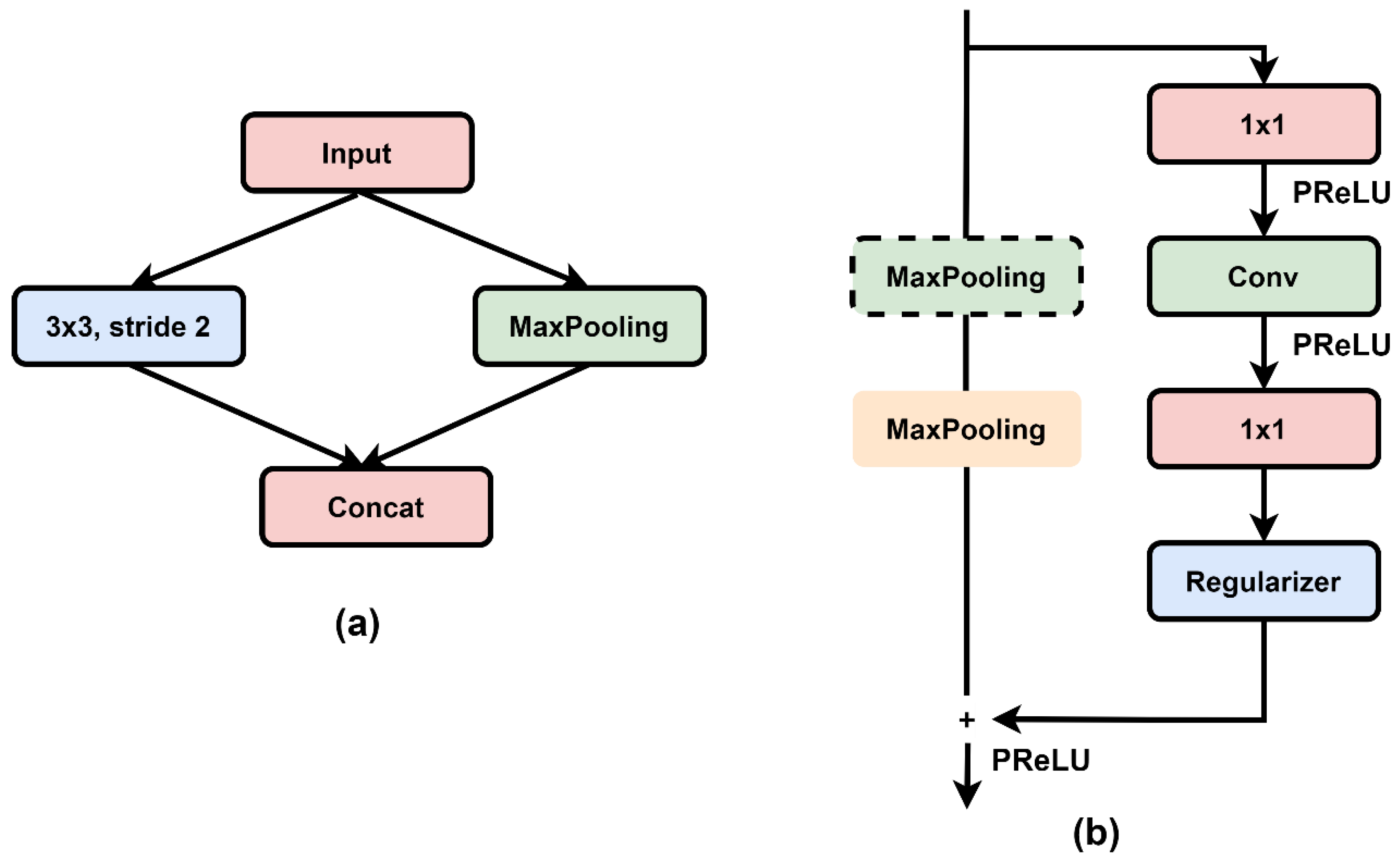
Figure 1. (a) ENet initial block; (b) ENet bottleneck module.
Applsci 12 12786 g001
Figure 2. Structure of CGblock used in the CGNet.
Applsci 12 12786 g002
Figure 3. Overall architecture of CGNet.
Applsci 12 12786 g003
Figure 4. Structure of (a) FCU block and (b) PFCU block.
Applsci 12 12786 g004
Figure 5. Overall symmetric encoder–decoder architecture of ESNet.
Applsci 12 12786 g005
Figure 6. Overall architecture of DDRNet-23-Slim.
Applsci 12 12786 g006
Figure 7. Overall architecture of DeepLabV3+ (Backbone Network = ResNet-50).
Applsci 12 12786 g007
Figure 8. Examples from concrete dataset with damage and respective ground truths (in colors).
Applsci 12 12786 g008
Figure 9. Example of prediction results of all models with original images and ground truths.
Applsci 12 12786 g009aApplsci 12 12786 g009b
Figure 10. Example of prediction results of all models in complex background conditions.
Applsci 12 12786 g010aApplsci 12 12786 g010b
Table 1. Evaluation results of all trained models corresponding to each damage class.
Damage ClassModelsPrecisionRecallF1 ScoreIoU
CracksENet0.58 0.71 0.64 (91.31) *0.45 (84.00) **
CGNet0.50 0.71 0.59 (84.09) * 0.42 (77.74) **
ESNet0.56 0.74 0.64 (91.61) *0.46 (86.77) **
DDRNet-23-Slim0.48 0.66 0.56 (80.24) *0.38 (70.75) **
DeepLabV3+0.62 0.79 0.70 (100.00) *0.54 (100.00) **
EfflorescenceENet0.76 0.67 0.71 (91.41) *0.55 (88.15) **
CGNet0.71 0.71 0.71 (91.69) *0.59 (94.54) **
ESNet0.81 0.61 0.69 (89.25) * 0.52 (82.25) **
DDRNet-23-Slim0.74 0.68 0.71 (90.96) *0.56 (89.63) **
DeepLabV3+0.81 0.75 0.78 (100.00) *0.63 (100.00) **
Rebar ExposureENet0.72 0.56 0.63 (85.26) *0.45 (77.01) **
CGNet0.68 0.62 0.65 (87.70) *0.47 (79.91) **
ESNet0.66 0.57 0.61 (82.86) *0.43 (74.32) **
DDRNet-23-Slim0.63 0.45 0.53 (70.98) *0.33 (57.01) **
DeepLabV3+0.77 0.72 0.74 (100.00) *0.58 (100.00) **
SpallingENet0.72 0.71 0.71 (91.55) *0.54 (83.90) **
CGNet0.77 0.72 0.75 (95.83) *0.61 (94.36) **
ESNet0.72 0.65 0.68(87.63) *0.51 (79.68) **
DDRNet-23-Slim0.75 0.65 0.70 (89.75) *0.52 (81.44) **
DeepLabV3+0.80 0.75 0.78 (100.00) *0.64 (100.00) **
* Ratio of F1 score of all models to DeepLabV3+. ** Ratio of IoU to DeepLabV3+.
Table 2. Computational cost comparison of all trained models.
Sr. NoModelsParameters
Millions (m)
FLOPs(G)Inference Speed
Milliseconds (ms)
1ENet0.46.98140
2CGNet0.59.860
3ESNet1.641.4296
4DDRNet-23-Slim5.716.2785
5DeepLabV3+17156.6780
Publisher’s Note: MDPI stays neutral with regard to jurisdictional claims in published maps and institutional affiliations.