Abstract
Deep neural networks (DNNs) require large amounts of labeled data for model training. However, label noise is a common problem in datasets due to the difficulty of classification and high cost of labeling processes. Introducing the concepts of curriculum learning and progressive learning, this paper presents a novel solution that is able to handle massive noisy labels and improve model generalization ability. It proposes a new network model training strategy that considers mislabeled samples directly in the network training process. The new learning curriculum is designed to measures the complexity of the data with their distribution density in a feature space. The sample data in each category are then divided into easy-to-classify (clean samples), relatively easy-to-classify, and hard-to-classify (noisy samples) subsets according to the smallest intra-class local density with each cluster. On this basis, DNNs are trained progressively in three stages, from easy to hard, i.e., from clean to noisy samples. The experimental results demonstrate that the accuracy of image classification can be improved through data augmentation, and the classification accuracy of the proposed method is clearly higher than that of standard Inception_v2 for the NEU dataset after data augmentation, when the proportion of noisy labels in the training set does not exceed 60%. With 50% noisy labels in the training set, the classification accuracy of the proposed method outperformed recent state-of-the-art label noise learning methods, CleanNet and MentorNet. The proposed method also performed well in practical applications, where the number of noisy labels was uncertain and unevenly distributed. In this case, the proposed method not only can alleviate the adverse effects of noisy labels, but it can also improve the generalization ability of standard deep networks and their overall capability.
1. Introduction
In recent years, deep neural networks (DNNs) have achieved tremendous success in various machine learning tasks, such as face recognition [1], image classification [2], etc. [3,4,5]. DNNs require large amounts of labeled data for model training. However, due to the difficulty of classification and high cost of the labeling process, label noise is a common problem in datasets. Although DNNs are somewhat robust to label noise [6], they tend to overfit the data, thus making them prone to memorizing even completely random noise. In order to efficiently train DNNs, the existence of label noise must be considered, and the corresponding algorithms must be developed to alleviate their adverse effects in model training.
In machine learning, noise contained in the training dataset can be divided into two categories: feature noise and label noise [7]. Feature noise corresponds to the corruption in observed data features, whereas label noise means the change in label from its true class. Both types of noise may cause a significant decrease in the performance of model training and classification. This study focused on the label noise, which is considered to have a greater impact on the performance of model training and classification than the feature noise. This is due to several factors: the label is unique for each data value, although features are multiple; and the importance of each feature varies, whereas the label always has a significant impact [8].
Label noise is unavoidable in application scenarios, and it is a natural consequence of the dataset collection process. Obtaining massive and clean annotators in application scenarios is expensive and time-consuming, especially for some professional datasets, in which expert knowledge is required and labels provided by different annotators may be inconsistent. Prior research has proven that noisy labels can significantly affect the performance of DNNs in image classification [9].
Several attempts have been made to solve the noisy data problem in the network training process through noisy label learning technologies and have been successfully applied to several application scenarios [10,11,12]. The techniques mainly include the methods that learn noisy labels directly and the semi-supervised methods which first train models on a small subset of clean labeled samples and then generalize the model trained on that subset to unlabeled or weakly labeled sample dataset. However, those methods may suffer from the problems of poor generalization ability, difficulties in identifying mislabeled samples from hard samples, and increased computational cost and training time.
Curriculum learning [13] is a sample choosing algorithm which was inspired by human cognition and proposes to start from easy samples and utilize harder samples to guide training. Curriculum learning can accelerate the training of machine learning models and enable the model to obtain a better generalization performance. Most contemporary curriculum learning methods are based on the framework design of the difficulty measurer and training scheduler. Among them, difficulty measurers determine the learning priority of each data value, and training schedulers determine when to input the hard data into training and how much to put in each time. Depending on whether the difficulty measurer and training scheduler can be designed automatically, curriculum learning can be divided into predefined curriculum learning and automatic curriculum learning. Image classification using DNNs requires the purification of the dataset as a preprocessing stage for model training: in this case, the concept of curriculum learning can be introduced to improve the model training performance. However, in curriculum learning, the specification of “easy samples” is achieved through the difficulty measurer, which is a task-specific issue. Moreover, when to input the hard data into training and how much to put in each time with the training scheduler is always hard to decide. It is often difficult to find the best combination of both difficulty measurer and training scheduler.
Progressive learning is a deep learning framework for continual learning [14]. The progression procedure is used to grow the model’s capacity by adding new parameters that leverage parameters learned in prior tasks, while learning from data available for the new task at hand, without being susceptible to catastrophic forgetting. It is shown that, when tasks are related, progressive learning leads to faster learning that converges to a better generalization performance, using a smaller number of dedicated parameters.
The motivation of this paper is to provide a new idea and method for solving noisy labels effectively. The generalization ability of standard deep networks and their overall capability are improved by introducing a new training strategy to alleviate the adverse effects of noisy labels on network model training. The method can also improve the accuracy of network classification and realize the needs of defect detection in the actual factories. The main contributions of this paper are as follows:
- A new network training strategy is proposed. Unlike previous research methods, we do not propose noise cleansing or noise robustness or semi-supervised algorithms, but a new network model training strategy that considers mislabeled samples directly in the network training process. This method can effectively alleviate the adverse effects of noisy labels on network model training and improve the accuracy of network classification without changing the architecture of standard deep networks.
- A new learning curriculum is designed to measure the complexity of the data by using the distribution density of the data in the feature space, and the complexity of the data is ranked in an unsupervised manner. The data are then divided into three subsets and input into the network “progressively” according to their complexity. This method provides a new idea of determining the “easy sample” in traditional curriculum learning and improves the generalization ability of the network.
- The proposed method can achieve better classification results in large-scale and high-complexity datasets, and it effectively improves the accuracy of defect classification in the case of uncertain and unevenly distributed mislabeled samples. The reliability and validity of the proposed model are proved by statistical analysis, and the practicality of the proposed method is verified by practical industrial application.
2. Preliminaries and Related Works
This section gives a brief review on recent studies developed for dealing with noisy labels on image classification. These mainly include methods that aim to directly learn from noisy labels; semi-supervised learning methods, which combine noisy labels with a small set of clean labels; and convolutional neural networks, which are applied to train a robust model with noisy data.
2.1. Methods Directly Learn from Noisy Labels
The methods aim to directly learn from noisy labels mainly include noise-robust algorithms and label-cleansing methods, which aim to remove or correct mislabeled data.
2.1.1. Robust Loss Function
The main idea of the robust loss function against noisy labels is that, when the data are generally clean, the traditional cross-entropy loss function learns a small number of negative samples, which can improve the robustness of the model. Conversely, when the proportion of noisy data is relatively large, the cross-entropy will be deviated by the noisy data, and the loss function needs to be modified to make the weight of each training sample equally important.
The main purpose of these methods is to provide a robust loss function so that, even if there are noisy labels in the training data, it can also bring a small risk to the clean samples. Ghosh et al. [15] proved that the loss function based on the mean absolute error (MAE) is inherently robust to label noise; therefore, standard back propagation is enough to learn the true classifier even under label noise. However, MAE may perform poorly with DNNs and challenging datasets. In order to solve this problem, Zhang et al. [16] presented a GCE loss, which can be seen as a generalization of MAE and categorical cross-entropy (CCE), and it achieved a good performance in a wide range of noisy label scenarios. In addition, inspired by the symmetric KL-divergence, Wang et al. [17] proposed a symmetric cross-entropy (RCE) approach, which can simultaneously address both the under-learning and overfitting problem of cross-entropy in the presence of noisy labels.
2.1.2. Robust Architecture
Robust architecture mainly learns the robustness of the model gradually during the model training process by borrowing an ingenious network structure. These structural changes include adding a noise adaptation layer on top of the softmax layer or designing a new dedicated architecture. The output of the DNNs is modified by basing it on the estimated probability of label transfer. A representative method is the co-teaching framework [18,19]. It maintains two networks simultaneously, and in each mini-batch data, each network samples its small-loss instances as the useful knowledge and teaches such useful instances to its peer network for further training.
2.1.3. Noise-Cleansing Method
Noise-cleansing methods screen the suspected noisy samples through active learning and then hand them over to human experts for relabeling. Based on this concept, Dauphin [20] proposed a noise-cleaning technique called the ensemble method based on the noise detection metric (ENDM). An ensemble classifier is first learned from the corrupted training set, and it is then used to derive four metrics for assessing the likelihood for a sample to be mislabeled. The thresholds of Bagging, AdaBoost, and KNN are used to identify and then either remove or correct the corrupted samples.
2.2. Semi-Supervised Learning
Semi-supervised learning is a method to reduce annotation cost in the case of labeled and unlabeled data. In order to overcome noisy labels, some recent studies have turned the problem of learning from noisy labels into a semi-supervised learning task. The semi-supervised learning method aims to improve the model’s performance by leveraging unlabeled data. Contemporary semi-supervised learning methods mainly regularize training by adding additional loss terms to unlabeled data. The regularization involves consistency regularization, which enforces the model to produce consistent predictions on augmented input data [21,22,23], or entropy minimization, which encourages the model to give high-confidence predictions on unlabeled data [24,25]. In this field of study, the samples that may have incorrect labels in the noisy data are re-graded as unlabeled samples, while the remaining samples are re-graded as labeled samples. Then the transformed data are used for semi-supervised learning. Li et al. [26] proposed a DividedMix method. It draws on the idea of co-training: after picking out clean samples and noisy samples, the noisy samples are re-graded as unlabeled samples and trained by the FixMatch method. Lee et al. [27] introduced a transfer learning approach, namely CleanNet, to solve label noise by transferring the correctness of labels to other classes.
2.3. Convolutional Neural Networks
Convolutional neural networks (CNNs) have recently been applied to training a robust model with noisy data. For example, Tong et al. [28] presented a general framework to train CNNs with a limited number of clean labels and millions of easily obtained noisy labels. They modeled the relationships between images, class labels, and label noises with a probabilistic graphical model and further integrated them into an end-to-end deep learning system. Jiang et al. [29] improved the performance of CNNs on noisy data by learning an additional network which weighs the training examples, called MentorNet, to supervise the training of the base deep networks.
3. Methodology
This section clarifies the motivation of the proposed method by analyzing the limitations of existing technologies. On this basis, the proposed methods are described in detail.
3.1. The Motivation
As mentioned in the previous section, a lot of research has been performed to deal with noisy labels on image classification, and the most representative are methods that learn noisy labels directly and the semi-supervised methods that use a small number of clean samples for training and then generalize the model trained on that subset to unlabeled or weakly labeled sample dataset. However, the main problem with methods that learn noisy labels directly is that they usually face the major challenge of identifying mislabeled samples from hard training samples; thus, fixing this issue is crucial for improving the model’s capabilities. This class of methods performs well only in simple cases, such as those where learning is easy or the number of classes is small. In addition, modifications to the loss function increase the training time for the model to converge. The semi-supervised techniques can significantly improve the noise robustness. However, hyperparameters introduced by these techniques make DNNs more susceptible to changes in data and noise types, and an increase in computational cost is inevitable.
Based on these merits and demerits of existing technologies, the motivation of the proposed method is to provide a new idea and method for solving noisy labels effectively. Unlike previous research methods, we do not propose noise cleansing or noise robustness or semi-supervised algorithms; instead, we propose a new network model training strategy that considers mislabeled samples directly in the network training process. This method can effectively alleviate the adverse effects of noisy labels on network model training and improve the accuracy of network classification without changing the architecture of standard deep networks. Moreover, a new learning curriculum is designed to measure the complexity of the data by using the distribution density of the data in the feature space, and the complexity of the data is ranked in an unsupervised manner. The data are then divided into three subsets and input into the network “progressively” according to their complexity. This method provides a new idea of determining the “easy sample” in traditional curriculum learning and improves the generalization ability of the network.
3.2. Overview
An overview of the proposed method is given in Figure 1. It mainly contains three steps: (1) initial feature extraction, (2) data complexity measurement, and (3) progressive model training. First, random samples from the sample dataset are chosen to pretrain the DNN, and all samples are fed into the trained model according to their categories for feature extraction. Second, the K-means algorithm is employed to divide the samples in each category into three clusters according to the product of the local density and distance; then samples in each category are divided into easy-to-classify, relatively easy-to-classify, and hard-to-classify subsets according to the smallest intra-class local density in each cluster. Third, data from the same subset of all categories are combined, and the data are fed into the DNN in order from easy to hard to progressively train the DNN in three stages. Thus, the model capacity can be gradually improved gradually by progressively adding increasingly complex data into the training process.
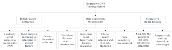
Figure 1.
An overview of the proposed method.
3.3. Initial Feature Extraction
Image classification by neural network is performed to input the image feature vector into the neural network model for processing and complete image classification according to the processing result. In this case, we conducted the following procedures:
Step 1: Initializing the DNN model by randomly selecting samples from the sample dataset to pretrain the DNN model.
Step 2: Inputting all samples according to categories into the trained model to extract features.
Step 3: Performing dimension reduction with PCA on extracted feature vectors to simplify the subsequent work.
3.4. Data Complexity Measurement
As mentioned in Section 1, the specification of easy samples in curriculum learning is a task-specific issue which may vary due to different tasks. The aim of this study was to design an approach that could rank the training images from easy to complex in a relatively unsupervised manner. This approach is inspired by the K-means algorithm, where the complexity of the training samples can be measured through the data distribution density. We assumed that by training a neural network, each class of samples can be mapped into a deep feature space. Higher local densities indicate more likely clean samples with correct labels, because they are often clustered together with a similar appearance. Conversely, samples with noisy labels have a small density, i.e., poor aggregation. In this case, we conduct the following procedures in each category:
Step 1: Set the training sample set as T, the number of sample categories as n, and the training sample dataset of the ith class as Ti, and Ti contains mi samples, . In Ti, we calculate the Euclidean distance between the jth sample feature vector and the 1st sample feature vector, and construct an intra-class Euclidean distance matrix:
where , , . Then, sorting the element in the intra-class Euclidean distance matrix to determine the median value .
Step 2: For the jth sample in the ith class, calculate its intra-class local density, :
where , and is the number of samples whose Euclidean distance between the feature vector in and the jth sample feature vector is less than . The larger indicates that, in the feature space, more samples are close to each other with the feature vector of the jth sample.
Step 3: For the jth sample in the ith class, calculating its intra-class distance is performed as follows:
when the jth sample of the ith class has the largest intra-class local density of the ith class, represents the largest value of the jth row of the distance matrix, ; otherwise, represents the distance between the sample point with the smallest distance from the jth sample point and the jth sample point among all the sample points in the ith class, whose intra-class local density is greater than the jth sample.
Step 4: Since the cluster center should have the largest value and the largest value at the same time [30], determining the cluster center involves calculating the product of the intra-class local density, , and the intra-class distance, :
Step 5: Sorting the value of the ith samples () in descending order, the feature vectors of the samples corresponding to the first three values are selected as the initial cluster center. The K-means algorithm is adopted to cluster the samples according to the Euclidean distance from the sample point to the cluster center in the feature space and obtain three clusters. Then, the intra-class local density of the samples is sorted into the three clusters, taking the smallest intra-class local density value in each cluster and sorting in descending order to obtain , , and , defining the jth sample , which satisfies as the easy-to-classify sample subset, ; the jth sample, which satisfies , is the relatively easy-to-classify sample subset, ; and the jth sample, which satisfies , is the hard-to-classify sample subset, .
3.5. Progressive Model Training
By defining the complexity of the data with their distribution density in a feature space, the model training starts with learning easy-to-classify samples (clean samples) and then progressively includes the relatively easy-to-classify and hard-to-classify samples (noisy samples) in the training process. The neural network is trained progressively from easy to hard to improve the performance of model training and classification. In this case, we conduct the following procedures:
Step 1: Combining the easy-to-classify subsets of all categories to obtain , combining the relatively easy-to-classify subsets of all categories to obtain , and combining the relatively easy-to-classify subsets of all categories to obtain :
where .
Step 2: Randomly initializing the DNN and using the samples in to train the initial DNN to obtain the first stage network model.
Step 3: Using the samples in and to train the first-stage network model to obtain the second-stage network model.
Step 4: Using the samples in , , and to train the second-stage network model to obtain the final model.
4. Experimental Results and Comparisons
In this section, the proposed method is evaluated on both the benchmark dataset NEU and a real-world steel surface defect detection case to demonstrate its effectiveness.
4.1. Experiments on the Benchmark Dataset NEU
In the surface-defects dataset of Northeast University (NEU) [31], six typical surface defects of hot-rolling steel strip were collected: crazing (Cr), inclusion (In), patches (Pa), pitted surface (PS), rolled-in scale (RS), and scratches (Sc). Each defect contained 300 labeled grayscale images with an original resolution of . Figure 2 shows examples of the defective images in NEU. The defects in the same columns belong to the intra-class defects, and the different columns belong to the inter-class defects. In the figure, it is clear that the inter-class divergence is small, but the intra-class divergence varies. However, the appearance of inter-class defects can be different; for example, the scratches may be horizontal, vertical, or slanting. Moreover, intra-class defects may also have similar aspects, such as the rolled-in scale, crazing, and pitted surfaces. In addition, due to the influence of illumination and material changes, the grayscale of the intra-class defect images varies.
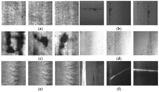
Figure 2.
Examples of defect images in NEU: (a) crazing (Cr), (b) inclusion (In), (c) patches (Pa), (d) pitted surface (PS), (e) rolled-in scale (RS), and (f) scratches (Sc).
The Inception_v2, which has been successfully adopted in previous studies, is an effective network for defects detection in the NEU dataset. In this case, we still took this network initially to compare and analyze the experimental results. The main advantage of the Inception network is that it changes the serial target detection network into a parallel computing mode, which can reduce the optimization parameters in the deep learning network, reduce the amount of computation, and optimize the computing speed.
During the experiment, it first randomly initializes the weight parameters of Inception_v2, and then it selects random samples from the sample dataset to pretrain the network. Then the softmax classifier layer is removed from the pretrained model to form a feature-extraction module, and a 2048-dimensional-feature vector is obtained by inputting all samples into the feature-extraction module by category. In order to reduce the amount of computation, PCA is adopted to reduce the dimension of the extracted 2048-dimensional-feature vector to obtain a 256-dimensional-feature vector, and then the 256-dimensional-feature vector is processed according to the method flow in Section 3.
Extensive experiments were conducted to evaluate the efficiency of the proposed method. We compared four training strategies, which are described as follows:
- Strategy 1: The model is trained with the standard Inception_v2 architecture and the proposed method with the original NEU dataset.
- Strategy 2: The model is trained with the standard Inception_v2 architecture and the proposed method with the NEU dataset after data augmentation.
- Strategy 3: The model is trained with standard Inception_v2 architecture and the proposed method with the increasing percentage of the noisy labels in training set.
- Strategy 4: The model is trained by the proposed method and recent state-of-the-art methods with the NEU dataset after data augmentation (50% noisy labels in training set).
4.1.1. The Performance of Progressive Learning in Clean Dataset
In this experiment, the NEU dataset was divided into a training set and a test set. The training set contained 1500 samples, and each defect retained 50 samples with truth labels, and the remaining labels were removed. The NEU dataset is a benchmark dataset; therefore, we assumed that all the samples are truth labels. All the hyperparameters were selected by cross-validation, and a summary of the Inception_v2 network is presented in Table 1. During the network training, the learning rate was set to 0.01, the batch_size was set to 36, and the max_step was set to 1000.

Table 1.
Details of Inception_v2.
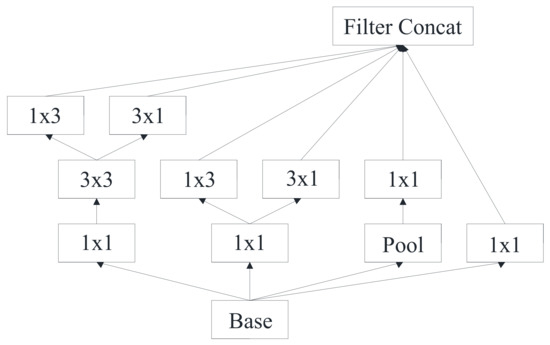
Figure 5.
The module.
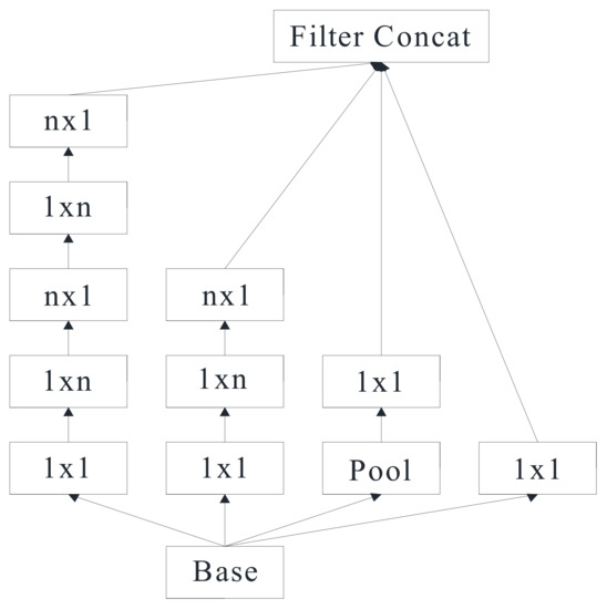
Figure 4.
The module.
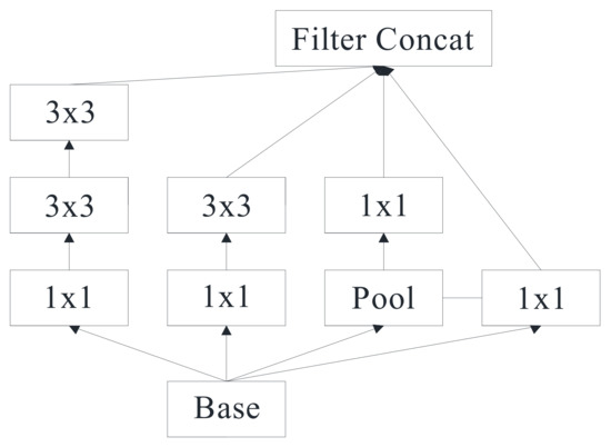
Figure 3.
The module.
Table 1.
Details of Inception_v2.
| Type | Patch Size/Stride | Input Size |
|---|---|---|
| Conv | 3 × 3/2 | 299 × 299 × 3 |
| Conv | 3 × 3/1 | 149 × 149 × 32 |
| conv padded | 3 × 3/1 | 147 × 147 × 32 |
| Pool | 3 × 3/2 | 147 × 147 × 64 |
| Conv | 3 × 3/1 | 73 × 73 × 64 |
| Conv | 3 × 3/2 | 71 × 71 × 80 |
| Conv | 3 × 3/1 | 35 × 35 × 192 |
| 3 × Inception | As in Figure 3 | 35 × 35 × 288 |
| 5 × Inception | As in Figure 4 | 17 × 17 × 768 |
| 2 × Inception | As in Figure 5 | 8 × 8 × 1280 |
| Pool | 8 × 8 | 8 × 8 × 2048 |
| Linear | Logits | 1 × 1 × 2048 |
| Softmax | Classifier | 1 × 1 × 1000 |
This experiment compared the performance of the standard Inception_v2 and the proposed progressive learning method on a clean dataset. The results are presented in Table 2. Before the comparison, the confusion matrix was introduced. A confusion matrix is a matrix used for assessing the performance of classifiers. The general idea of a confusion matrix is to compute the number of instances of Class A which are classified as Class B. A confusion matrix produces a lot of information, which can be summarized as follows:
- False negative (FN) is the outcome where the model incorrectly predicts the negative class.
- True negative (TN) is the outcome the model correctly predicts the negative class.
- False positive (FP) is the outcome where the model incorrectly predicts the positive class.
- True positive (TP) is the outcome where the model correctly predicts positive class.
Accuracy is the most common metric used to evaluate the performance of a classification model. The recognition accuracy is calculated as follows:
Table 2.
The average classification accuracies of standard Inception_v2 and the proposed method with the original NEU dataset.
Table 2.
The average classification accuracies of standard Inception_v2 and the proposed method with the original NEU dataset.
| Original NEU Dataset | ||
|---|---|---|
| Accuracy (%) | Standard Inception_v2 | 86.55 |
| Proposed method | 83.79 | |
It can be seen from Table 2 that the average classification accuracies of the standard Inception_v2 and proposed method are 86.55% and 83.79%, respectively. Although the proposed method can still obtain high classification accuracy, compared with the standard Inception_v2, the accuracy is not significantly improved. One possible explanation is that labels in the original NEU dataset are clean labels, and a standard Inception_v2 is sufficient to improve the defect classification accuracy through simple network training when the dataset is relatively small. Meanwhile, PCA for the proposed method for dimensionality reduction may lose some information, even though it will speed up network training.
4.1.2. The Effects of Training Data Volume/Complexity
In this experiment, the original NEU dataset was enlarged to 9000 samples by adopting data-augmentation methods (e.g., flipping and add Gaussian noise). The training set contained 5400 samples, and the validation set and test set contained 1800 samples. The example images after data augmentation are shown in Figure 6. For comparison purposes, the hyperparameter settings are the same as in the previous section.
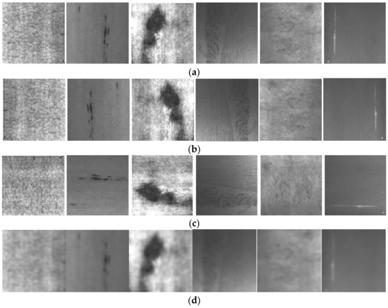
Figure 6.
Example images after data augmentation: (a) the original images, (b) images after flipping 180°, (c) images after flipping 90°, and (d) images after adding Gaussian noise (radius = 3).
The average defect classification accuracies of a standard Inception_v2 architecture and the proposed method with the original NEU dataset and the NEU dataset after data augmentation are compared in Table 3. It can be seen by comparing Table 3 and Table 2 that the classification accuracy was improved through data augmentation for both the standard Inception_v2 and the proposed method. Moreover, in Table 3, the defects classification accuracy of the proposed method is relatively higher than that of the standard Inception_v2. A reasonable explanation is that, after data augmentation, the dataset volume increases and the features are more complex, which may provide more information for network learning; the results also demonstrate the strong robustness of the proposed method in a large-scale complex dataset.
Table 3.
The average classification accuracies of standard Inception_v2 and the proposed method with the NEU dataset after data augmentation.
Besides accuracy, the specificity and sensitivity are also two main statistical metrics to evaluate the performance of the model. The specificity represents the proportion of the negative samples that were correctly classified, and the sensitivity is the proportion of the positive samples that were correctly classified. The specificity and sensitivity are calculated as follows:
Table 4 provides the accuracy, sensitivity, and specificity of each defect of the proposed model. It can be seen from the table that the proposed model has both high defects classification sensitivity and specificity, so the results of the proposed method are significant, and the proposed method is effective.
Table 4.
The accuracy, sensitivity, and specificity of each defect of proposed method with the NEU dataset after data augmentation.
4.1.3. The Effects of Increasing the Percentage of Noisy Labels in the Training Set
In this experiment, noisy labels were artificially added to the training set of the NEU dataset after data augmentation by adopting the following steps:
Step 1: According to the given noise ratio (percentage of noisy labels), namely NoiseLevel, select K samples from N total samples:
Step 2: For each category of samples in the selected K samples, replace its original label with a random number between 0 and 6 (six typical steel surface defects) after deducting the original label (i.e., the truth label).
Figure 7 shows the trends in defects classification accuracy of standard Inception_v2 and the proposed method when the proportion of noisy labels in the training set increases from 0% to 100%. It can be observed from the figure that even the standard Inception_v2 can maintain the classification accuracy of the test set above 80% when the percentage of noisy labels in the training set does not exceed 60%. The most plausible explanation for this is that the labels are basically uniformly distributed in the NEU dataset. For each label, the original label was replaced with one of the other five random numbers, the noisy labels were evenly distributed among the other five categories, and the number of truth labels was significantly higher than the number of noisy labels. When the percentage of noisy labels increased further, although the percentage of truth labels was still higher than that of the noisy labels, the quantitative advantages started to be reduced. We calculated the current truth labels in one category and the noisy labels distributed in other categories by increasing the percentage of noisy labels; the results are shown in Table 5.
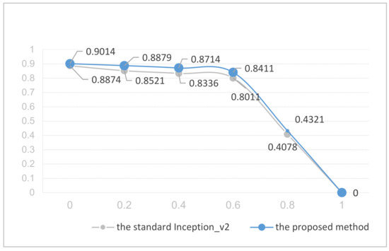
Figure 7.
The trends in classification accuracy of standard Inception_v2 and the proposed method.
Table 5.
The truth labels in one category and the noisy labels are distributed to other categories.
It can be observed from the table that the classification accuracy of proposed method is considerably higher than that of the standard Inception_v2 when the percentage of noisy labels does not exceed 60%. When the percentage of noisy labels exceeds 60%, the classification accuracy of both standard inception_v2 and the proposed method drop rapidly. The results demonstrate the strong robustness of the proposed method in the presence of noisy labels in model training. In actual production, more than 85% of the defect classification accuracy is required. The standard inception_v2 barely meets the requirement when the percentage of noisy labels in the training set reaches 20% and fails to meet the requirement when it exceeds 20%; however, the proposed method can meet the requirement well when the percentage of noisy labels reaches 40% and even maintains a classification accuracy higher than 85% when the percentage of noisy labels exceeds 50%.
4.1.4. Comparisons with Recent State-of-the-Art Methods
The proposed method was evaluated by comparing it with recent state-of-the art methods specifically developed for learning from label noise, i.e., CleanNet [27] and MentorNet [29]. The experimental objects of both the CleanNet and MentorNet comparison methods are different from the experimental objects of this paper: for better comparison, the NEU dataset after augmentation was used as the basic experimental dataset for all three methods in this experiment. In CleanNet and MentorNet, we reset the hyperparameters according to the characteristics and quantities of the input data. At the same time, in order to validate the effect of noisy labels in the training set on these three methods, we set the percentage of noisy labels in training set as 50%. The reason for this is that, in actual production, a defect classification of more than 85% is required, and we proved in Figure 7 that the proposed method can maintain a classification accuracy above 85% when the percentage of noisy labels does not exceed 50%. The full results are presented in Table 6.
Table 6.
Comparisons with recent state-of-the-art label noise learning methods.
It can be seen from the table that the classification accuracies with 50% noisy labels of CleanNet and MentorNet are 81.33% and 82.44%. The accuracy of the proposed method was improved by 4.9% from the best result in the comparison methods.
4.2. Experiments on a Real-World Case
The proposed method was applied to solve a real-world steel-surface defects-detection case. We assessed a Chinese real-world cold-rolling steel workshop which produces elector-galvanized steel strips for vehicles. The flowchart of the production is shown in Figure 8. Statistically, the qualified rate of this production is only 78.6%, and more than 95.4% of defects occur on the surface. An automatic surface inspection (ASI) system was set up, and defect images were collected. In the early stages, the workshop had already carried out some degree of intelligent defect detection. Support vector machine (SVM) algorithms were applied to classify the defects, but the recognition accuracy was less than 70%, and at least 85% was required in this workshop.
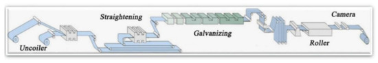
Figure 8.
The flowchart of production in a real-world case.
In order to improve the recognition accuracy, 25,000 defect images with six typical defects were provided, and 3000 of these images were manually labeled, i.e., rolling marks, sliver, edge defect, scratches, and hole. Examples of collected images are shown in Figure 9. For a better comparison, we also adopted Inception_v2 for the experiments. This paper demonstrates the noise immunity of the progressive learning method to noisy labels. In this case, we only compared the recognition accuracy and FP rate, which are the two most important indicators for the workshop.
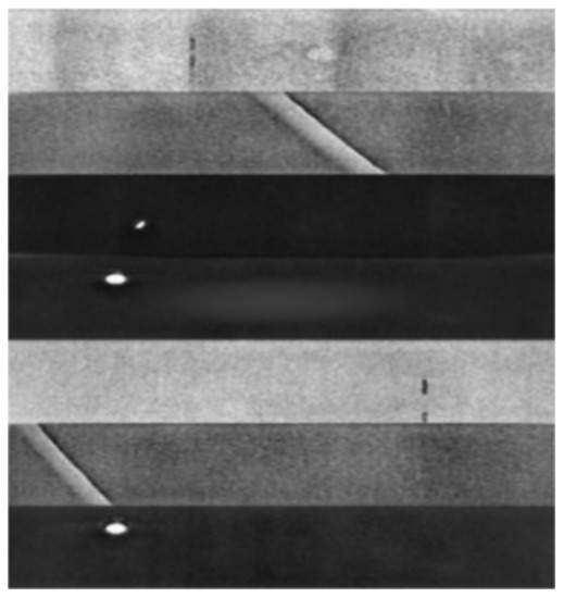
Figure 9.
Examples of the collected images.
In addition to accuracy, the FP rate reflects the ability of the classification model to correctly predict the purity of positive samples in order to reduce the number of negative samples predicted as positive, i.e., the proportion of negative samples predicted as positive to the total number of negative samples. The FP rate is calculated as follows:
The comparison results are presented in Table 7. From the table, it is clear that the proposed method outperforms the standard Inception_v2 in terms of accuracy and FP rate, especially for the rolling marks, hole, and edge defects. For the proposed method, the classification accuracy is slightly lower, and the FP rate is slightly higher than other defects in cracks and scratches. A possible explanation for this is the similarity in the features of cracks and scratches, which are sometimes difficult to distinguish.
Table 7.
Comparison of defect recognition accuracy.
In practical applications, the number of noisy labels is uncertain and unevenly distributed. In this case, the results also demonstrate that the proposed method can improve the accuracy of network model training to some extent, thus improving the effectiveness of defect classification.
4.3. Lessons Learned
We summarize the key observations of the experiments as follows: (1) A standard Inception_v2 architecture was sufficient to improve the defect classification accuracy through simple network training when the dataset is relatively small. (2) Data augmentation can improve the classification accuracy of the model with a certain range. (3) The proposed method has strong robustness in a large-scale complex dataset, which has important implications for practical applications. (4) A standard Inception_v2 architecture can maintain the classification accuracy at a high level with a relatively low percentage of noisy labels if the labels are basically uniformly distributed in the dataset. (5) The classification accuracy of the proposed method is clearly higher than that of the standard Inception_v2 when the percentage of noisy labels does not exceed 60%; however, when the percentage of noisy labels exceeds 60%, the classification accuracy of both the standard Inception_v2 and the proposed method drops rapidly. (6) With 50% noisy labels, the classification accuracy of the proposed method outperforms the recent state-of-the-art label noise learning methods: CleanNet and MentorNet. (7) The proposed method can perform well in practical applications, where the number of noisy labels is uncertain and not necessarily uniformly distributed. This was proven through a steel surface defect detection case in a Chinese real-world cold-rolling steel workshop.
4.4. Findings and Further Analysis
(1) In this paper, a new network training strategy was proposed. Unlike previous research methods, this paper proposed a new network model training strategy that considers mislabeled samples directly in the network training process. The experimental results demonstrated that this method can effectively alleviate the adverse effects of noisy labels on model training and improve the accuracy of network classification without changing the architecture of standard deep networks. However, in this paper, only Inception_v2 network was adopted for comparison. Further analysis should focus on investigating the superior performance of proposed method on other classical deep neural networks.
(2) In this paper, a new learning curriculum was designed to measure the complexity of the data by using the distribution density of the data in the feature space, and the complexity of the data was ranked in an unsupervised manner. The data were then divided into three subsets, namely easy-to-classify samples (clean samples), relatively easy-to-classify samples, and hard-to-classify samples (noisy samples), and input into the network “progressively” according to their complexity. Further analysis should focus on investigating whether dividing samples into more subsets according to the complexity of the data can achieve a better classification performance.
(3) We proved that the proposed method can achieve a state-of-the-art performance on the benchmark dataset and a real-world defect detection case through statistical analysis. However, the selection of hyperparameters of the network and the image quality of the initial experiments may affect the training and performance of the network. Further analysis should focus on conducting more experiments to verify the significance of the proposed method.
5. Conclusions
This paper has proposed a new model training method, namely the progressive DNN training method, which aims to provide a new idea and method for solving noisy labels effectively. We evaluated our proposed method on both the benchmark dataset and a real-world steel surface defect detection case to demonstrate its effectiveness. The experimental results demonstrate that data augmentation can improve the classification accuracy of the model within a certain range, and the classification of the proposed method is demonstrably higher than that of standard Inception_v2 on the NEU dataset after data augmentation when the percentage of noisy labels in the training set does not exceed 60%. With 50% noisy labels in the training set, the classification accuracy of the proposed method outperforms the contemporary state-of-the-art label noise learning methods: CleanNet and MentorNet. The proposed method can also perform well in practical applications, where the number of noisy labels is uncertain and unevenly distributed. In this case, the generalization ability of standard deep networks and their overall capability can be improved by introducing this method to alleviate the adverse effects of noisy labels on network model training. The method can also improve the accuracy of network classification and realize the needs of defect detection in the actual factories. The proposed method could be further improved through comparing other classical deep neural networks, dividing samples into more subsets, and conducting more experiments to verify its prior performance.
Author Contributions
Conceptualization, X.Y. and L.W.; methodology, X.Y.; software, Z.Z.; validation, X.Y., X.X. and L.W.; formal analysis, X.X.; investigation, L.W.; resources, X.Y.; data curation, Z.Z.; writing—original draft preparation, X.Y.; writing—review and editing, Z.Z.; visualization, X.X.; supervision, L.W.; project administration, Z.Z.; funding acquisition, X.Y. All authors have read and agreed to the published version of the manuscript.
Funding
This research was funded by the National Natural Science Foundation of China (grant 52205537).
Institutional Review Board Statement
Not applicable.
Informed Consent Statement
Informed consent was obtained from all subjects involved in the study.
Data Availability Statement
Not applicable.
Conflicts of Interest
The authors declare no conflict of interest.
References
- Liyew, B.T. Applying a Deep Learning Convolutional Neural Network (CNN) Approach for Building a Face Recognition System: A Review. J. Emerg. Technol. Innov. Res. 2017, 4, 1104–1110. [Google Scholar]
- Dani, S.; Hanwate, P.S.; Panse, H.; Chaudhari, K.; Kotwal, S. Survey on the use of CNN and Deep Learning in Image Classification. J. Emerg. Technol. Innov. Res. 2021, 8, 609–611. [Google Scholar]
- Yoo, J.; Lee, C.H.; Jea, H.M.; Lee, S.K.; Yoon, Y.; Lee, J.; Hwang, S.U. Classification of Road Surfaces Based on CNN Architecture and Tire Acoustical Signals. Appl. Sci. 2022, 12, 9521. [Google Scholar] [CrossRef]
- Alghamdi, H.S. Towards Explainable Deep Neural Networks for the Automatic Detection of Diabetic Retinopathy. Appl. Sci. 2022, 12, 9435. [Google Scholar] [CrossRef]
- Guo, L.; Ding, S. A hybrid deep learning CNN-ELM model and its application in handwritten numeral recognition. J. Comput. Inf. Syst. 2015, 11, 2673–2680. [Google Scholar]
- Nayereh, G.; Baraani, D.A. Semi-Automatic Labeling of Training Data Sets in Text Classification. Comput. Inf. Sci. 2011, 4, 48–56. [Google Scholar]
- Shanthini, A.; Vinodhini, G.; Chandrasekaran, R.M.; Supraja, P. A taxonomy on impact of label noise and feature noise using machine learning technique. Soft Comput. 2019, 23, 8597–8607. [Google Scholar] [CrossRef]
- Algan, G.; Ulusoy, I. Image classification with deep learning in the presence of noisy labels: A survey. Knowl. -Based Syst. 2021, 215, 106771. [Google Scholar] [CrossRef]
- Ahmed, A.; Yousif, H.; He, Z. Ensemble diversified learning for image classification with noisy labels. Multimed. Tools Appl. 2021, 80, 20759–20772. [Google Scholar] [CrossRef]
- Ji, D.; Oh, D.; Hyun, Y.; Kwon, O.M.; Park, M.J. How to handle noisy labels for robust learning from uncertainty. Neural Netw. 2021, 143, 209–217. [Google Scholar] [CrossRef] [PubMed]
- Nicholson, B.; Sheng, V.S.; Zhang, J. Label noise correction and application in crowdsourcing. Expert Syst. Appl. 2016, 66, 149–162. [Google Scholar] [CrossRef]
- Gu, N.; Fan, M.; Meng, D. Robust Semi-Supervised Classification for Noisy Labels Based on Self-Paced Learning. IEEE Signal Process Lett. 2016, 23, 1806–1810. [Google Scholar] [CrossRef]
- Patrini, G.; Rozza, A.; Krishna Menon, A.; Nock, R.; Qu, L. Making deep neural networks robust to label noise: A loss correction approach. In Proceedings of the 2017 IEEE Conference on Computer Vision and Pattern Recognition, Honolulu, HI, USA, 21–26 July 2017; pp. 1944–1952. [Google Scholar]
- Hendrycks, D.; Mazeika, M.; Wilson, D.; Gimpel, K. Using trusted data to train deep networks on labels corrupted by severe noise. In Proceedings of the 32nd International Conference on Neural Information Processing Systems, Montréal, QC, Canada, 3–8 December 2018; pp. 10456–10465. [Google Scholar]
- Ghosh, A.; Kumar, H.; Sastry, P.S. Robust Loss Functions under Label Noise for Deep Neural Networks. In Proceedings of the Thirty-First AAAI Conference on Artificial Intelligence, San Francisco, CA, USA, 4–9 February 2017; pp. 1919–1925. [Google Scholar]
- Zhang, Z.; Sabuncu, M.R. Generalized Cross Entropy Loss for Training Deep Neural Networks with Noisy Labels. In Proceedings of the 32nd Conference on Neural Information Processing Systems, Montréal, QC, Canada, 2–8 December 2018; pp. 8778–8788. [Google Scholar]
- Wang, Y.; Ma, Y.; Chen, Y.; Luo, Y.; Yi, J.; Bailey, J. Symmetric Cross Entropy for Robust Learning with Noisy Labels. In Proceedings of the 2019 IEEE International Conference on Computer Vision, Seoul, South Korea, 27 October–3 November 2019; pp. 322–330. [Google Scholar]
- Yu, X.; Han, B.; Yao, J.; Niu, G.; Tsang, I.W.; Sugiyama, M. How does Disagreement Help Generalization against Label Corruption? In Proceedings of the 2019 International Conference on Machine Learning, Long Beach, NY, USA, 10–16 June 2019; pp. 7164–7173. [Google Scholar]
- Han, B.; Yao, Q.; Yu, X.; Niu, G.; Xu, M.; Hu, W.; Tsang, I.W.; Sugiyama, M. Co-teaching: Robust Training of Deep Neural Networks with Extremely Noisy Labels. In Proceedings of the 32nd Conference on Neural Information Processing Systems, Montréal, QC, Canada, 2–8 December 2018; pp. 8536–8546. [Google Scholar]
- Dauphin, G. Label Noise Cleaning with an Adaptive Ensemble Method Based on Noise Detection Metric. Sensors 2020, 20, 6718. [Google Scholar] [CrossRef] [PubMed]
- Laine, S.; Aila, T. Temporal Ensembling for Semi-Supervised Learning. In Proceedings of the 2017 International Conference on Learning Representation, Toulon, France, 24–26 April 2017. [Google Scholar]
- Tarvainen, A.; Valpola, H. Mean teachers are better role models: Weight-averaged consistency targets improve semi-supervised deep learning results. In Proceedings of the 2017 Conference and Workshop on Neural Information Processing Systems, Long Beach, CA, USA, 21–26 July 2017; pp. 1195–1204. [Google Scholar]
- Miyato, T.; Maeda, S.I.; Koyama, M.; Ishii, S. Virtual adversarial training: A regularization method for supervised and semi-supervised learning. IEEE Trans. Pattern Anal. Mach. Intell. 2019, 41, 1979–1993. [Google Scholar] [CrossRef] [PubMed]
- Grandvalet, Y.; Bengio, Y. Semi-supervised learning by entropy minimization. In Proceedings of the 2004 Neural Information Processing System, Vancouver, BC, Canada, 13–18 December 2004; pp. 529–536. [Google Scholar]
- Lee, D.H. Pseudo-label: The simple and efficient semi-supervised learning method for deep neural networks. ICML Workshop Chall. Represent. Learn. 2013, 3, 2. [Google Scholar]
- Li, J.; Socher, R.; Hoi, S.C.H. DivideMix: Learning with Noisy Labels as Semi-supervised Learning. In Proceedings of the International Conference on Learning Representations, Online. 26–30 April 2020. [Google Scholar]
- Lee, K.H.; He., X.; Zhang, L.; Yang, L. CleanNet: Transfer Learning for Scalable Image Classifier Training with Label Noise. In Proceedings of the 2018 IEEE/CVF Conference on Computer Vision and Pattern Recognition, Salt Lake City, UT, USA, 18–21 June 2018. [Google Scholar]
- Tong, X.; Tian, X.; Yi, Y.; Chang, H.; Wang, X. Learning from massive noisy labeled data for image classification. In Proceedings of the 2015 IEEE Conference on Computer Vision and Pattern Recognition, Boston, MA, USA, 7–12 June 2015. [Google Scholar]
- Jiang, L.; Zhou, Z.; Leung, T.; Li, L.; Li, F. MentroNet: Learning Data-Driven Curriculum for Very Deep Neural Networks on Corrupted Labels. In Proceedings of the 2018 International Conference on Machine learning, Stockholm, Sweden, 10–15 July 2018. [Google Scholar]
- Gu, H. Application and research of distance and density on improved k- means application and research of distance and density on improved k-means. J. Phys. Conf. Ser. 2019, 1168, 32135. [Google Scholar] [CrossRef]
- Song, K.; Yan, Y. A noise robust method based on completed local binary patterns for hot-rolled steel strip surface defects. Appl. Surf. Sci. 2013, 285, 858–864. [Google Scholar] [CrossRef]
Publisher’s Note: MDPI stays neutral with regard to jurisdictional claims in published maps and institutional affiliations. |
© 2022 by the authors. Licensee MDPI, Basel, Switzerland. This article is an open access article distributed under the terms and conditions of the Creative Commons Attribution (CC BY) license (https://creativecommons.org/licenses/by/4.0/).