Support Vector Machine-Assisted Importance Sampling for Optimal Reliability Design

Abstract

A population-based optimization algorithm combining the support vector machine (SVM) and importance sampling (IS) is proposed to achieve a global solution to optimal reliability design. The proposed approach is a greedy algorithm that starts with an initial population. At each iteration, the population is divided into feasible/infeasible individuals by the given constraints. After that, feasible individuals are classified as superior/inferior individuals in terms of their fitness. Then, SVM is utilized to construct the classifier dividing feasible/infeasible domains and that separating superior/inferior individuals, respectively. A quasi-optimal IS distribution is constructed by leveraging the established classifiers, on which a new population is generated to update the optimal solution. The iteration is repeatedly executed until the preset stopping condition is satisfied. The merits of the proposed approach are that the utilization of SVM avoids repeatedly invoking the reliability function (objective) and constraint functions. When the actual function is very complicated, this can significantly reduce the computational burden. In addition, IS fully excavates the feasible domain so that the produced offspring cover almost the entire feasible domain, and thus perfectly escapes local optima. The presented examples showcase the promise of the proposed algorithm.

1. Introduction

There are various approaches to increase system reliability [1], for example, raising component reliability, increasing redundancy level, exchanging positions of important components, selection of different redundancy methods (e.g., active vs. standby), maintenance, etc. These measures undoubtedly will increase the system budget. Therefore, there needs to be a trade-off between reliability improvement and system budget [2]. No matter which measure we choose to enhance system reliability, the corresponding problem can be abstracted into a similar mathematical model, i.e., either maximizing system reliability under various resource constraints, or minimizing resource requirement under minimum reliability requirements. Of course, different methods of increasing system reliability correspond to different design variables, and the expression of system reliability is also different. Practically, we have to choose the most appropriate of one or several measures to improve system reliability according to the problem at hand. Another problem associated with this is how to procure the optimal decision scheme according to the established mathematical model.

There is a common sense that almost all optimal reliability designs (ORDs) are nondeterministic polynomial hard (NP-hard) problems [3]. Canonical methods for optimization, such as the linear/dynamic programming techniques, often fail or reach local optima in solving high-dimensional and complex problems. These are usually referred to as the exact methods. Although much more computational complexity is involved, exact methods are able to provide precise optimal solutions. These approaches are particularly advantageous for small-scale systems. More importantly, their solutions can be used to measure the performance of newly developed optimization strategies. Hence, there are also some improved versions of this kind of algorithm [4]. The difficulties associated with applying the mathematical programming on large-scale engineering systems have contributed to the development of alternative solutions.

One of the alternatives is the heuristic approach. Heuristics do not guarantee precise optimal solutions, but are highly recommended for solving ORD. This is because heuristics achieve reasonable solution quality for large-scale systems within relatively short periods [5]. Interestingly, heuristics usually leverage the sort information obtained by importance measures to guide the search direction. Importance measures, evaluating the relative importance of different components/positions in a system, can be used to prioritize components/positions in a system by quantitatively measuring their impact amount on the system reliability, whose value may not be as useful as their relative ranking [6]. The application of importance measures will guide the convergent direction and limit the randomness in heuristics, so that they can reach the (near) global optimal solution sooner. The role of importance measures in system design has been proved to be crucial. The heuristic approach is more efficient than the exact method, but it still takes a long time if the problem’s scale is very large.

To further accelerate the convergence speed, researchers have turned their attention to intelligent algorithms (i.e., metaheuristics). These are generally stochastic search methods that mimic the metaphor of natural biological evolution, social behavior of species, and natural/physical phenomena. Metaheuristics are currently considered to be the most promising solutions, because they can find (near) optimal solutions within reasonable CPU time. An old intelligent algorithm is simulated annealing (SA), which is invented on the basis of annealing (slow cooling after heating) of melted metals to crystallize their structures [7]. SA can jump out of the local optimum with a certain probability, and eventually tends to the global optimum. For applications of SA to solve ORD, we refer to [8,9]. Another well-known intelligent algorithm is the genetic algorithm (GA). GA is an evolutionary-based optimization technique, which was proposed by mimicking the natural selection and genetic mechanism [10]. Selection, crossover, and mutation are cores of GA. Examples of papers applying GA to solve ORD are [11,12,13]. Particle swarm optimization (PSO) is a random search algorithm based on group cooperation [14]. PSO is initialized as a group of random particles within the feasible domain. In each iteration, the particles update themselves by tracking the optimal solution found by the particle itself (i.e., individual best or personal best) and the optimal solution found by the whole population (i.e., global best). For papers that apply PSO to solve ORD, see [15,16,17]. Ant colony optimization (ACO) is a probabilistic algorithm used to find the optimal decision scheme [18]. It utilizes the walking path of ants to represent the feasible solution of the optimization problem. For applications of ACO for solving ORD, see [19,20]. There are also some other metaheuristics for solving ORD, such as in [21,22].

Nonconvex optimization problems can present many discontinuous discrete feasible regions and local optima. This may trap the algorithm’s iterations and make the algorithm of poor quality to tackle the problem at hand. Therefore, global optimization methods must be sought to escape local optima. Revisiting the collected literature, we can see intuitively that most population-based intelligent approaches are greedy algorithms. These explore the optimal solution gradually and iteratively. The decision of each iteration is usually made according to a certain criterion based on the current situation, without considering all possible situations. It makes successive greedy choices until the optimal solution is emerged. In this process, the generation (or renewal) of the next-generation population (or particle position, etc.) is a crucial operation. For example, SA draws new candidate solutions by simulating an ergodic Markov chain whose stationary distribution is the target distribution; GA produces new individuals through selection, crossover, and mutation; and PSO updates the positions of particles in terms of particle velocity, local optimum, and global optimum. Despite the benefits of intelligent algorithms, there are still many issues associated with implementing these approaches. For example, it is difficult to determine the initial temperature and temperature gradient in SA; GA may require long processing for a feasible solution to evolve; and PSO is easy to be caught into local optima and lacks of strict mathematical study.

In an attempt to reduce the processing time and improve the quality of solutions, particularly to escape local optima, this paper proposes a new population-based greedy algorithm that is able to reach the (near) global optimum in a relatively short time. The key ingredients of the proposed algorithm include importance sampling (IS) [23] and support vector machine (SVM) [24,25]. Starting from an initial group of individuals uniformly generated from the design domain, a new population is produced based on the existing information about the feasible/infeasible domains and the fitness values of feasible individuals. New populations will be generated iteratively until the optimal solution appears. To generate the new population in each iteration, a quasi-optimal IS probability density function (PDF) is constructed as the target distribution to draw samples for the new-generation population, leveraging the information of the constraint boundary and the fitness values of feasible individuals. To alleviate the computational burden, SVM is utilized to manage the information that is used to construct IS PDF, so as to avoid repeatedly invoking the objective and constraint functions numerous times. Obviously, this advantage is of great significant for complex problems. Furthermore, to speed up the convergence, a number of candidate solutions are generated at each iteration. The merits of the proposed algorithm are twofold. On the one hand, IS prevents sample degeneracy (keeps the sample diversity), and thus the exploration of the feasible space is more adequate. In addition, the constructed optimal IS PDF perfectly avoids local optima. On the other hand, the utilization of SVM escapes the repeated invocation of complex functions, thus saving computation time. This advantage is evident if the investigated problem involves complicated black-box functions.

The innovations and contributions of this paper are threefold. (a) A deterministic target distribution is constructed by utilizing IS without the need to set a series of parameters. (b) SVM is used to construct alternative models for dividing the feasible/infeasible domains and distinguishing the superior/inferior individuals. This facilitates the sampling process, because it does not need to repeatedly invoke the complex functions involved in the optimization model. (c) New individuals can be simply generated via the constructed quasi-optimal IS PDF without complicated operations. The diversity of new individuals is ensured and local optima avoided. The rest of this paper is organized as follows. Section 2 revisits the mathematical model related to ORD. Section 3 introduces the proposed algorithm with explanations of the rationale behind it. Numerical results are given in Section 4 to showcase the feasibility of the proposed algorithm. Conclusions are drawn in Section 5.

2. Model Description

In the light of the requirements of designers, ORD can be formulated either to maximize the system reliability under resource constraints or to minimize the resource under the minimum demand on system reliability. For brevity, we only take the former to illustrate. For the latter, the proposed algorithm is also applied. Put more clearly, the mathematical model of ORD is given by [26]:

$$\begin{array}{l}\underset{\mathit{z}}{\max :}{R}_s\left(\mathit{z}\right)\\ \mathrm{s}.\mathrm{t}. G_i\left(\mathit{z}\right)\le G_i^t (i=1,2,\cdots ,n_c)\\ {\mathit{z}}^L\le \mathit{z}\le {\mathit{z}}^U\end{array}$$

(1)

where $R_s\left(\mathit{z}\right)$ is the objective function (system reliability) related to design variables $\mathit{z}$. $G_i\left(\mathit{z}\right)$ is the $i$th constraint function with preset threshold $G_i^t$ for $i=1,2,\cdots ,n_c$, and $n_c$ is the number of constraints. ${\mathit{z}}^L$ and ${\mathit{z}}^U$ are the lower and upper bound vectors of decision variables $\mathit{z}$.

Example 1.

Takethe Wi-Fi system shown in Figure 1to illustrate. The whole area is covered by three signal networks, namely, Verizon, AT&T, and T-Mobile. Each carrier has four relay stations, and each relay station can send and receive signals in a specific block. Here, each block is covered by three consecutive staggered relay stations operated by these three carriers. The Wi-Fi system uses the strongest detection signals from different carriers. Unequivocally, the Wi-Fi signal loss in a particular area occurs if and only if the three consecutive staggered relay stations fail altogether. This Wi-Fi system can be abstracted into a Lin/Con/$k$/$n$:F system where $k=3$ and$n=12$. The Lin/Con/$k$/$n$:F system is a special two-terminal network that includes an ordered sequence of $n$components arranged in a line. The system fails if and only if at least $k$consecutive components fail. The Lin/Con/$k$/$n$:F system is important and has many applications, such as the pipeline system, streetlight system, and telecommunications system.

To improve the reliability of this Wi-Fi system, we can increase the reliability of relay station or the number of relay stations. Without loss of generality, we consider a Lin/Con/$k$/$n$:F system with redundant components, as shown in Figure 2, in which ${\mathit{z}}_j$ is the number of redundant components of the $j$th subsystem for $j=1,2,\cdots ,n$, and $n$ is the number of subsystems. The system fails if the successive $k$ subsystems fail. In this example, subsystem $j$ contains an active-standby component and ${\mathit{z}}_j-1$ cold-standby redundant components.

Suppose that the switch is required at all times, and there is a constant probability that the switching will be successful [8]. In addition, the following assumptions are made. (1) Each component/switch possesses only two states: normal and abnormal. (2) The performance of each component/switch is not affected by others. (3) There is no repair/maintenance during the whole service cycle. (4) The components or switches of a subsystem are of the same type. (5) There is imperfect switching to activate the cold-standby redundant components. (6) The time to failure of components is exponential.

Then, following [27,28], the reliability of subsystem $j$ is:

$$R_j\left(t\right)=r_j\left(t\right)+{\displaystyle \sum }_{s=1}^{z_j-1}{\int }_0^t{\rho }_j\left(u\right)r_j\left(t-u\right)f_j^{\left(s\right)}\left(u\right)du \left(j=1,2,\cdots ,n\right)$$

(2)

where $r_j\left(t\right)$ is the component reliability at moment $t$ for the $j$th subsystem, i.e., the probability that the lifetime of the component in the $j$th subsystem is larger than $t$. ${\rho }_j\left(t\right)$ is the reliability of the switching mechanism at moment $t$. $f_j^{\left(s\right)}\left(u\right)$ is the PDF for the $s$th failure in the $j$th subsystem, i.e., the probability that the $s$th failure in the $j$th subsystem arrives at moment $u$.

The first term of (2) indicates that the active-standby redundant component remains in a good state until moment $t$; during this period, no cold-standby redundant components are put into operation. The summation term in (2) represents $s$ cold-standby redundant components being sequentially activated through the switch. This implies that the initial active-standby redundant component and the first $s-1$ cold-standby redundant components have failed before moment $t$, and the $s$th cold-standby redundant component works until moment $t$. There are $s$ failures arriving in total, and all the $s$ switches are required to be successful to make sure that the system is reliable at moment $t$.

However, it is difficult to derive the closed form of (2), because of the intractability of the integration. A more accessible lower bound ${\underset{\_}{R}}_j\left(t\right)$ of the concerned reliability is given in [27] based on the non-increasing property of the switch device probability (i.e., ${\rho }_j\left(u\right)\ge {\rho }_j\left(t\right) \mathrm{for} u\le t$):

$$R_j\left(t\right)\ge {\underset{\_}{R}}_j\left(t\right)=r_j\left(t\right)+{\rho }_j\left(t\right){\displaystyle \sum }_{s=1}^{{\mathit{z}}_j-1}{\int }_0^t{r}_j\left(t-u\right)f_j^{\left(s\right)}\left(u\right)du \left(j=1,2,\cdots ,n\right)$$

(3)

Obviously, ${\underset{\_}{R}}_j\left(t\right)$ is a conservative estimation of $R_j\left(t\right)$. When ${\rho }_j\left(t\right)$ is close enough to 1, (3) is a good estimation of (2). For brevity, we no longer distinguish between $R_j\left(t\right)$ and ${\underset{\_}{R}}_j\left(t\right)$. Henceforth, unless otherwise specified, the system reliability refers to its lower bound.

Since the switch’s reliability is a constant, (3) can be simplified as:

$$R_j\left(t\right)=r_j\left(t\right)+{({\rho }_j)}^{{\mathit{z}}_j-1}{\displaystyle \sum }_{s=1}^{{\mathit{z}}_j-1}{\int }_0^t{r}_j\left(t-u\right)f_j^{\left(s\right)}\left(u\right)du \left(j=1,2,\cdots ,n\right)$$

(4)

where ${\rho }_j$ is the reliability of switches in subsystem $j$.

In terms of the exponential time-to-failure assumption, the occurrences of subsystem failures can be treated as a homogeneous Poisson process prior to the ${\mathit{z}}_j$th failure. On this basis, the reliability of subsystem $j$ is the probability that there are strictly less than ${\mathit{z}}_j$ failures, which is Poisson-distributed [27,29,30]. Therefore:

$${\int }_0^t{r}_j\left(t-u\right)f_j^{\left(s\right)}\left(u\right)du=\frac{{\left({\beta }_{j}t\right)}^s\exp \left(-{\beta }_{j}t\right)}{s!}$$

(5)

where ${\beta }_j$ is the component failure rate (the exponential distribution parameter) of the $j$th subsystem.

Taking (5) into (4), we can obtain:

$$R_j\left(t\right)=r_j\left(t\right)+{({\rho }_j)}^{{\mathit{z}}_j-1}{\displaystyle \sum }_{s=1}^{{\mathit{z}}_j-1}\frac{{\left({\beta }_{j}t\right)}^s\exp \left(-{\beta }_{j}t\right)}{s!} \left(j=1,2,\cdots ,n\right)$$

(6)

After that, the reliability of this Lin/Con/$k$/$n$:F system is obtained by the recursive function, as follows:

$$R_s\left(t;k,n\right)={\displaystyle \sum }_{i=n-k+1}^n{R}_i\left(t\right)R_s\left(t;k,i-1\right){\displaystyle \prod }_{j=i+1}^n\left(1-R_j\left(t\right)\right)$$

(7)

with the boundary condition $R_s\left(t;k,n\right)=1$ for $n<k$.

Now, the goal is to design a Lin/Con/$k$/$n$:F system under system-level constraints, such that the system reliability (7) is maximized. For simplicity, the design variables are temporarily set as redundant levels here, that is, $\mathit{z}=\left\{z_1,z_2,\cdots ,z_n\right\}$. Then, the mathematical model of this design task is as follows:

$$\begin{array}{l}\underset{\mathit{z}}{\max :}\left(7\right)\\ \mathrm{s}.\mathrm{t}. G_1\left(\mathit{z}\right)={\displaystyle {\displaystyle \sum }_{i=1}^n}(c_i{\mathit{z}}_i^2+{\mathit{z}}_i|\cos \left(\pi r_i\right)|)-C\le 0\\ G_2\left(\mathit{z}\right)={\displaystyle {\displaystyle \sum }_{i=1}^n}{v}_i{\mathit{z}}_i-V\le 0\\ {\mathit{z}}_i^L\le {\mathit{z}}_i\le {\mathit{z}}_i^U \left({\mathit{z}}_i\in {\mathbb{N}}_{+}, i=1,2,\cdots ,n\right)\end{array}$$

(8)

where $G_1\left(\mathit{z}\right)$ and $G_2\left(\mathit{z}\right)$ are cost and volume constraints, respectively, $c_i$ and $v_i$ are parameters related to these two constraints, respectively. $C$ and $V$ are the thresholds of these two constraints, respectively, $r_i$ is the reliability of component of subsystem $i$, $\mathrm{and} {\mathbb{N}}_{+}$ is the set of positive integers. In addition, these constraints are dimensionless and can be regarded as the constraints after standardization.

It is seen that (8) involves a complex system reliability function related to decision variables. To explore the optimal decision scheme, the recursive approach is usually adopted to estimate the system reliability under each candidate decision. However, for a candidate solution, it spends a long time on the recursion to procure a precise estimate. This will consume large computational effort and reduce the efficiency of the whole optimization procedure. To mitigate the computation burden, we propose an SVM-assisted IS approach to address the formulated ORD.

3. Proposed Solution Procedure

To facilitate understanding, we use (1) to illustrate the proposed population-based optimization algorithm. Following custom, we first transform (1) into a minimization problem, as follows:

$$\begin{array}{l}\underset{\mathit{z}}{\min :}H\left(\mathit{z}\right)=-R_s\left(\mathit{z}\right)\\ \mathrm{s}.\mathrm{t}. G_i\left(\mathit{z}\right)\le G_i^t (i=1,2,\cdots ,n_c)\\ {\mathit{z}}^L\le \mathit{z}\le {\mathit{z}}^U\end{array}$$

(9)

Here, $H\left(\mathit{z}\right)$ is the new objective function.

The general process of the population-based greedy approach for exploring the optimal solution of (9) is presented in Algorithm 1, in which $l$ stands for the $l$th iteration and $Ite{r}_{m\mathit{a}x}$ is the longest iteration time.

Algorithm 1 General process of the population-based optimization approach
1.	Produce the first-generation population.
	For $l=1:Ite{r}_{m\mathit{a}x}$:
2.	Sift out feasible individuals from the whole population.
3.	Record/update the current optimal solution.
4.	Evaluate the fitness values of feasible solutions.
5.	Produce the next-generation population.
	End for

The first-generation individuals are usually generated by evenly occupying the whole design space, in order to capture more information of the feasible domain and procure a relatively good solution at the initial design stage. To achieve this goal, we can use stratified sampling approaches, such as Latin hypercube sampling or low-discrepancy sampling strategies, such as Sobol’s sequence.

Then, we process the initial population, and the given constraints are utilized to filter out infeasible individuals while retain feasible ones. The current optimal solution is updated as the feasible individual with minimum objective function value. After that, a new-generation population should be produced with the intention of improving the solution. Before this, a criterion, dubbed the fitness, is usually used to evaluate existing feasible individuals, so as to determine the informative parent individuals (i.e., superior individuals) for the next generation. These superior individuals may be directly inherited by the offspring or act as guidelines to produce better offspring. Then, we process the new population with the same strategy of processing the previous population, in order to further refine the solution. This process is proceeded iteratively until the termination criterion or the limited maximum iteration number ($Ite{r}_{m\mathit{a}x}$) is achieved.

From the above analyses, it is seen that step 5 is at the core of the whole optimization approach, i.e., the way to produce the next-generation population is the key ingredient of the optimization algorithm. The quality of the offspring severely affects the quality of the final solution and the convergence speed of the algorithm. Generally, we hope that the new population has the following peculiarities: (i) falling within the feasible region as far as possible; (ii) mining the information of the feasible domain as much as possible; and (iii) possessing better fitness than their parents. These are the directions of the proposed approach to improve the efficacy of population-based approaches. Obviously, for the desired feature #i, we need to resort to constraint functions $G_i\left(\mathit{z}\right)$ ($i=1,2,\cdots ,n_c)$, because they decide whether an individual is feasible. For feature #ii, new individuals tend to be produced as evenly as possible in the feasible area, in order to fully mine the information of the feasible domain and escape local optima. As for #iii, we turn to current feasible individuals for help, striving to make new individuals better than their parents. In order to produce better offspring, the first idea that comes to mind is to straightforwardly generate new individuals in terms of the given proposal (or target) distribution. As such, the problem is transformed into how to establish a suitable proposal distribution to generate excellent offspring.

Motivated by these facts, we propose a new way to produce the offspring by drawing upon the principle of IS and SVM. The merits of the proposed algorithm can be explained from two perspectives. From the sampling perspective, the proposed algorithm helps to overcome sample degeneracy and keep the diversity of individuals, and ensures that each individual is informative. From the optimization perspective, the proposed algorithm brings more exploration to the neighborhood of good candidate solutions. It pays equal attention to possible solution spaces, rather than focusing only on elite parents, in order to perfectly avoid local optima. This advantage is very important for the problem of multiple discrete feasible regions, especially when the importance of each feasible region is close.

3.1. Importance Sampling for Optimal Proposal Distribution

Let $f\left(\mathit{z}\right)$ be the prior joint PDF of variables $\mathit{z}$, and $g\left(\mathit{z}\right)$ be the PDF of the needed proposal distribution. Then, for any integrable function $\phi \left(\mathit{z}\right)$, its integration with respect to $f\left(\mathit{z}\right)$ equals:

$$I_{\phi }={\displaystyle \int }\phi \left(\mathit{z}\right)f\left(\mathit{z}\right)d\mathit{z}$$

(10)

Taking advantage of the instrumental PDF $g\left(\mathit{z}\right)$, (10) can be equivalently expressed as:

$$I_{\phi }={\displaystyle \int }\phi \left(\mathit{z}\right)\frac{f\left(\mathit{z}\right)}{g\left(\mathit{z}\right)}g\left(\mathit{z}\right)d\mathit{z}=\mathbb{E}\left(\frac{f\left(\mathit{z}\right)}{g\left(\mathit{z}\right)}\phi \left(\mathit{z}\right)\right)$$

(11)

If we draw $N$ independent and identically distributed (i.i.d.) samples ${\left\{{\mathit{z}}_i\right\}}_{i=1}^N$ from $g\left(\mathit{z}\right)$ and set their weights ${\left\{{\omega }_i\right\}}_{i=1}^N$ according to:

$${\varpi }_i=\frac{f\left({\mathit{z}}_i\right)}{g\left({\mathit{z}}_i\right)}$$

(12)

Then, in view of (11), the estimate of $I_{\phi }$ is:

$${\widehat{I}}_{\phi }=\frac{1}{N}{\displaystyle \sum }_{i=1}^N{\varpi }_i\phi \left({\mathit{z}}_i\right)$$

(13)

This instrumental PDF $g\left(\mathit{z}\right)$ is also referred to as the IS PDF corresponding to $f\left(\mathit{z}\right)$. A most direct IS PDF $g\left(\mathit{z}\right)$ is to transfer the sampling center from the mean point to an informative point, as shown in Figure 3. In Figure 3, it is a 2D case in the standard normal space. The dashed lines stand for the iso-probability density lines of $f\left(\mathit{z}\right)$ or $g\left(\mathit{z}\right)$. The mean point of $f\left(\mathit{z}\right)$ is the origin, and the sampling center of $g\left(\mathit{z}\right)$ is ${\mathit{z}}^{\ast }$. Now, suppose that subspace 1 is the region of interest (e.g., feasible domain), while subspace 2 is a region of no concern (e.g., infeasible domain). There is a boundary separating these two spaces. The purpose of sampling is to place samples in subspace 1 as much as possible. Obviously, $f\left(\mathit{z}\right)$ cannot complete this goal, but $g\left(\mathit{z}\right)$ can. This IS PDF is easy to understand, but its defects are evident. If a problem has multiple informative points and the importance of each informative point is close, this IS will be trapped into local optima, but for a practical problem, we cannot know whether it has multiple informative points in advance. For the investigated problem, the informative point can be viewed as a local optimal solution. Thus, we need to explore a more suitable IS strategy that globally explores the interested domain.

It is seen that the expectation of estimate ${\widehat{I}}_{\phi }$ is:

$$\mathbb{E}\left({\widehat{I}}_{\phi }\right)=\mathbb{E}\left(\frac{1}{N}{\displaystyle \sum }_{i=1}^N{\varpi }_i\phi \left({\mathit{z}}_i\right)\right)=\mathbb{E}\left(\frac{1}{N}{\displaystyle \sum }_{i=1}^N\frac{f\left({\mathit{z}}_i\right)}{g\left({\mathit{z}}_i\right)}\phi \left({\mathit{z}}_i\right)\right)=\frac{1}{N}{\displaystyle \sum }_{i=1}^N\mathbb{E}\left(\frac{f\left({\mathit{z}}_i\right)}{g\left({\mathit{z}}_i\right)}\phi \left({\mathit{z}}_i\right)\right)$$

(14)

Since ${\left\{{\mathit{z}}_i\right\}}_{i=1}^N$ are i.i.d. samples from $g\left(\mathit{z}\right)$, (14) can be further transformed into:

$$\mathbb{E}\left({\widehat{I}}_{\phi }\right)=\mathbb{E}\left(\frac{f\left({\mathit{z}}_i\right)}{g\left({\mathit{z}}_i\right)}\phi \left({\mathit{z}}_i\right)\right)=\mathbb{E}\left(\frac{f\left(\mathit{z}\right)}{g\left(\mathit{z}\right)}\phi \left(\mathit{z}\right)\right)=I_{\phi }$$

(15)

This indicates that (13) is an unbiased approximation of $I_{\phi }$.

Then, the variance of estimate ${\widehat{I}}_{\phi }$ is:

$$\mathbb{V}\left({\widehat{I}}_{\phi }\right)=\mathbb{V}\left(\frac{1}{N}{\displaystyle \sum }_{i=1}^N{\varpi }_i\phi \left({\mathit{z}}_i\right)\right)=\mathbb{V}\left(\frac{1}{N}{\displaystyle \sum }_{i=1}^N\frac{f\left({\mathit{z}}_i\right)}{g\left({\mathit{z}}_i\right)}\phi \left({\mathit{z}}_i\right)\right)=\frac{1}{N^2}{\displaystyle \sum }_{i=1}^N\mathbb{V}\left(\frac{f\left({\mathit{z}}_i\right)}{g\left({\mathit{z}}_i\right)}\phi \left({\mathit{z}}_i\right)\right)$$

(16)

In the same vein, due to ${\left\{{\mathit{z}}_i\right\}}_{i=1}^N$ are i.i.d. samples from $g\left(\mathit{z}\right)$, $\mathbb{V}({\widehat{I}}_{\phi })$ can be converted into:

$$\mathbb{V}\left({\widehat{I}}_{\phi }\right)=\frac{1}{N}\mathbb{V}\left(\frac{f\left({\mathit{z}}_i\right)}{g\left({\mathit{z}}_i\right)}\phi \left({\mathit{z}}_i\right)\right)=\frac{1}{N}\mathbb{V}\left(\frac{f\left(\mathit{z}\right)}{g\left(\mathit{z}\right)}\phi \left(\mathit{z}\right)\right)$$

(17)

Because the variance of samples converges to that of the population in the sense of probability, we can obtain:

$$\begin{array}{c}\mathbb{V}\left(\frac{f\left(\mathit{z}\right)}{g\left(\mathit{z}\right)}\phi \left(\mathit{z}\right)\right)\approx \frac{1}{N-1}\left[{\displaystyle {\displaystyle \sum }_{j=1}^N}{\left(\frac{f\left({\mathit{z}}_j\right)}{g\left({\mathit{z}}_j\right)}\phi \left({\mathit{z}}_j\right)\right)}^2-N{\mathbb{E}}^2\left(\frac{f\left(\mathit{z}\right)}{g\left(\mathit{z}\right)}\phi \left(\mathit{z}\right)\right)\right]\\ =\frac{N}{N-1}\left[\frac{1}{N}{\displaystyle {\displaystyle \sum }_{j=1}^N}{\left(\frac{f\left({\mathit{z}}_j\right)}{g\left({\mathit{z}}_j\right)}\phi \left({\mathit{z}}_j\right)\right)}^2-{\left(\frac{1}{N}{\displaystyle {\displaystyle \sum }_{i=1}^N}\frac{f\left({\mathit{z}}_i\right)}{g\left({\mathit{z}}_i\right)}\phi \left({\mathit{z}}_i\right)\right)}^2\right]\\ =\frac{N}{N-1}\left[\frac{1}{N}{\displaystyle {\displaystyle \sum }_{j=1}^N}{\left(\frac{f\left({\mathit{z}}_j\right)}{g\left({\mathit{z}}_j\right)}\phi \left({\mathit{z}}_j\right)\right)}^2-{\widehat{I}}_{\phi }^2\right]\end{array}$$

(18)

Substituting (18) for (17), $\mathbb{V}({\widehat{I}}_{\phi })$ can be approximated by:

$$\mathbb{V}({\widehat{I}}_{\phi })\approx \frac{1}{N-1}\left[\frac{1}{N}{\displaystyle \sum }_{j=1}^N{\left(\frac{f\left({\mathit{z}}_j\right)}{g\left({\mathit{z}}_j\right)}\phi \left({\mathit{z}}_j\right)\right)}^2-{\widehat{I}}_{\phi }^2\right]$$

(19)

Reducing the variance $\mathbb{V}({\widehat{I}}_{\phi })$ to 0, we can obtain:

$$g_{opt}\left(\mathit{z}\right)=\frac{\phi \left(\mathit{z}\right)f\left(\mathit{z}\right)}{I_{\phi }}=\frac{\phi \left(\mathit{z}\right)f\left(\mathit{z}\right)}{\int \phi \left(\mathit{z}\right)f\left(\mathit{z}\right)d\mathit{z}}$$

(20)

where $g_{opt}\left(\mathit{z}\right)$ is the optimal choice of $g\left(\mathit{z}\right)$, i.e., optimal IS PDF.

This optimal IS PDF $g_{opt}\left(\mathit{z}\right)$ no longer provides the maximum priority for a certain point, but assigns priority depending on the contribution of the point itself to the solution. Its advantages are escaping from local optima and avoiding searching for the important point of constructing IS PDF.

Figure 4a shows a 2D problem with multiple important points (regions), and the shaded area represents the region of interest. It is seen that this example possesses discrete interested domains that look like a chessboard. If we use the IS shown in Figure 3 to sample for the interested domains, a possible result is shown in Figure 4b. It can be observed that a vast majority of samples are concentrated in a local area. If the best solution is in this local area, this case can happen to get the global optimum. However, if the global optimum is far away from this region, it is obvious that this case is caught in the local optimum. Figure 4c presents the sampling result obtained by the optimal IS PDF $g_{opt}\left(\mathit{z}\right)$. Compared with Figure 4b, the generated samples cover multiple regions of interest. Therefore, it explores feasible regions more fully, and the possibility of obtaining the global optimal solution is obviously larger.

Now, recall that our purpose is to produce new individuals within the feasible domain that have better fitness than their parents. Let $I_F\left(\mathit{z}\right)$ be an indicator function such that $I_F\left(\mathit{z}\right)=1$ if $\mathit{z}$ belongs to the feasible domain, $I_F\left(\mathit{z}\right)=0$ otherwise. Furthermore, let $I_{\lambda }\left(\mathit{z}\right)$ be the indicator function such that $I_{\lambda }\left(\mathit{z}\right)=1$ if $H\left(\mathit{z}\right)\le \lambda$, $I_{\lambda }\left(\mathit{z}\right)=0$ otherwise. $\lambda$ is a constant that is related to the fitness. For two feasible individuals, ${\mathit{z}}_i$ and ${\mathit{z}}_j$, if $H\left({\mathit{z}}_i\right)\le H\left({\mathit{z}}_j\right)$, we say that the fitness of ${\mathit{z}}_i$ is better than that of ${\mathit{z}}_j$. Feasible individuals that satisfy $H\left(\mathit{z}\right)\le \lambda$ are referred to as superior individuals, and those with $H\left(\mathit{z}\right)>\lambda$ are inferior individuals.

After that, we clarify the specific form of $\phi \left(\mathit{z}\right)$ as:

$$\phi \left(\mathit{z}\right)=I_F\left(\mathit{z}\right)I_{\lambda }\left(\mathit{z}\right)$$

(21)

Here, $\phi \left(\mathit{z}\right)$ stands for an indicator function so that $\phi \left(\mathit{z}\right)=1$ if $\mathit{z}$ is a feasible point with objective function value smaller than $\lambda$, and $\phi \left(\mathit{z}\right)=0$ otherwise.

Using (21), the optimal proposal distribution (20) can be further expressed as:

$$g_{opt}\left(\mathit{z}\right)=\frac{I_F\left(\mathit{z}\right)I_{\lambda }\left(\mathit{z}\right)f\left(\mathit{z}\right)}{\int I_F\left(\mathit{z}\right)I_{\lambda }\left(\mathit{z}\right)f\left(\mathit{z}\right)d\mathit{z}}$$

(22)

Sampling from $g_{opt}\left(\mathit{z}\right)$ theoretically can obtain the optimal desired offspring. However, this optimal IS PDF $g_{opt}\left(\mathit{z}\right)$ is not available in practice, because we do not have any information of the feasible domain in advance. That is, $I_F\left(\mathit{z}\right)$ is unknown and should be explored. Meanwhile, we need to determine the threshold value $\lambda$, in order to determine $I_{\lambda }\left(\mathit{z}\right)$. Hence, we can only integrate the current available information to establish an asymptotical alternative to the optimal IS PDF $g_{opt}\left(\mathit{z}\right)$, in order to generate offspring according to the proposal distribution. Obviously, the current information we have is that from parent populations. The indicator function $I_F\left(\mathit{z}\right)$ is unknown, but we can construct an alternative model ${\widehat{I}}_F\left(\mathit{z}\right)$ for it by leveraging the available information of the feasible/infeasible domains. In the same vein, the alternative model ${\widehat{I}}_{\lambda }\left(\mathit{z}\right)$ for $I_{\lambda }\left(\mathit{z}\right)$ can be also established through the data set including superior individuals (with $H\left(\mathit{z}\right)\le \lambda$) and inferior individuals ($H\left(\mathit{z}\right)>\lambda$). Then, an asymptotical model ${\widehat{g}}_{opt}\left(\mathit{z}\right)$ for $g_{opt}\left(\mathit{z}\right)$ is constructed as follows:

$${\widehat{g}}_{opt}\left(\mathit{z}\right)=\frac{{\widehat{I}}_F\left(\mathit{z}\right){\widehat{I}}_{\lambda }\left(\mathit{z}\right)f\left(\mathit{z}\right)}{\int {\widehat{I}}_F\left(\mathit{z}\right){\widehat{I}}_{\lambda }\left(\mathit{z}\right)f\left(\mathit{z}\right)d\mathit{z}}\propto {\widehat{I}}_F\left(\mathit{z}\right){\widehat{I}}_{\lambda }\left(\mathit{z}\right)f\left(\mathit{z}\right)$$

(23)

where ${\widehat{g}}_{opt}\left(\mathit{z}\right)$ is also referred to as the quasi-optimal IS PDF.

The remaining issue is how to construct the alternative models ${\widehat{I}}_F\left(\mathit{z}\right)$ and ${\widehat{I}}_{\lambda }\left(\mathit{z}\right)$. To construct the alternative model for $I_F\left(\mathit{z}\right)$, we utilize the existing feasible and infeasible individuals as the training data set. Meanwhile, the alternative model for $I_{\lambda }\left(\mathit{z}\right)$ is constructed by using two sets of feasible individuals: the one set contains feasible individual with objective function value larger than $\lambda$ (inferior individuals), and the other set has feasible individual with objective function value smaller than $\lambda$ (superior individuals). The alternative models are constructed by SVM using data sets, since these two tasks are binary-classification problems and SVM is good at handling such problems. In the following section, we first showcase a brief review of SVM. Then, the concrete procedures for constructing the alternative models ${\widehat{I}}_F\left(\mathit{z}\right)$ and ${\widehat{I}}_{\lambda }\left(\mathit{z}\right)$ via SVM are presented.

3.2. SVM for Alternative Model

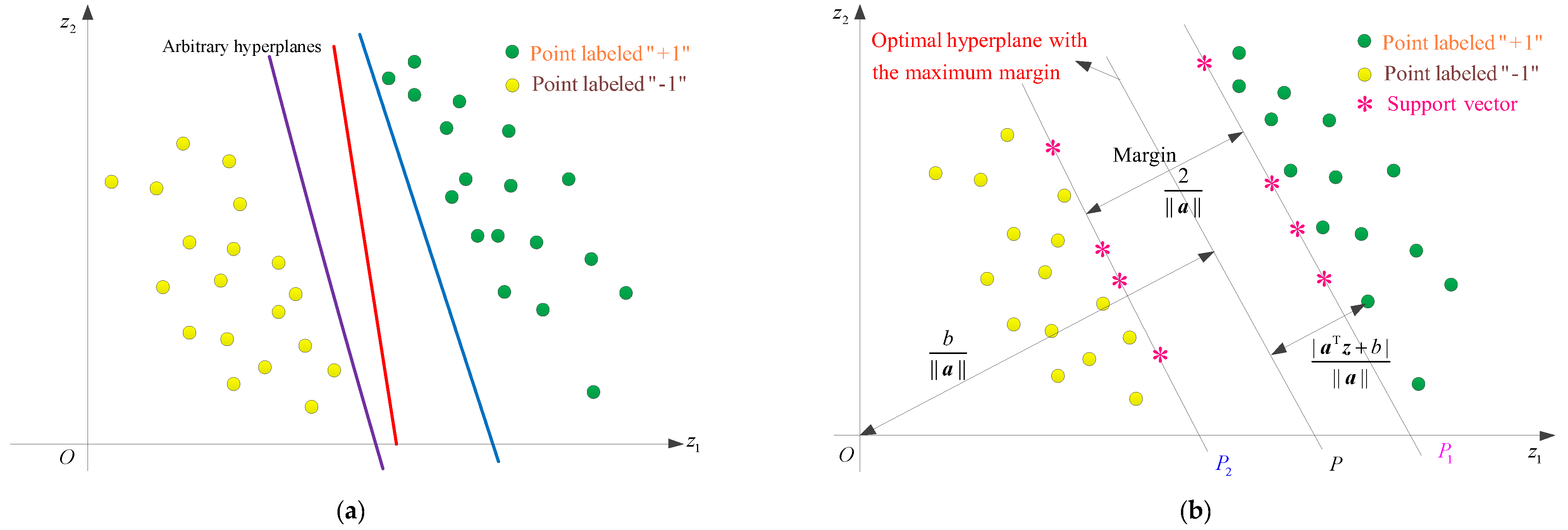
Given a binary-classification problem, let $\mathbb{D}=\{({\mathit{z}}_i^{\left(t\right)},y_i^{\left(t\right)}),i=1,2,\cdots ,N_t\}$ be the set of labeled training data, where ${\mathit{z}}_i^{\left(t\right)}$ is the ith training sample, $y_i^{\left(t\right)}\in \left\{-1,1\right\}$ is the label of ${\mathit{z}}_i^{\left(t\right)}$, and $N_t$ is the number of training samples. SVM aims to search for an optimal decision hyperplane for which all points labeled “−1” are located on one side and all points labeled “+1” on the other side [24]. As shown in Figure 5, Figure 5a shows arbitrary hyperplanes that can distinguish two types of samples, while Figure 5b represents the optimal classification hyperplane.

A possible hyperplane that divides a sample space into two types of subspaces is:

$$P: {\mathit{a}}^{\mathrm{T}}\mathit{z}+b=0$$

(24)

where the weight vector $\mathit{a}$ is perpendicular to the hyperplane, and b is a scalar parameter that represents the bias.

To determine $\mathit{a}$ and b, so as to orientate the hyperplane to be as far as possible from the closest samples, two hyperplanes ($P_1$ and $P_2$) parallel to decision boundary $P$ are as follows:

$$P_1: {\mathit{a}}^{\mathrm{T}}\mathit{z}+b=+1, P_2: {\mathit{a}}^{\mathrm{T}}\mathit{z}+b=-1$$

(25)

There are no points between $P_1$ and $P_2$. The shortest distance from the decision boundary ($P$) to $P_1/P_2$ is $1/\left|\left|\mathit{a}\right|\right|$, thus the margin between $P_1$ and $P_2$ is $2/\left|\left|\mathit{a}\right|\right|$. All training points $\mathbb{D}$ should satisfy $y_i^{\left(t\right)}({\mathit{a}}^{\mathrm{T}}{\mathit{z}}_i^{\left(t\right)}+b)\ge 1$. Therefore, determining the optimal hyperplane $P$ with maximum margin is equivalently reduced to finding $P_1$ and $P_2$ that give the maximum margin, as follows:

$$\begin{array}{l}\min : \frac{1}{2}{\left|\left|\mathit{a}\right|\right|}^2\\ \mathrm{s}.\mathrm{t}. y_i^{\left(t\right)}({\mathit{a}}^{\mathrm{T}}{\mathit{z}}_i^{\left(t\right)}+b)\ge 1 (i=1,2,\cdots ,N_t)\end{array}$$

(26)

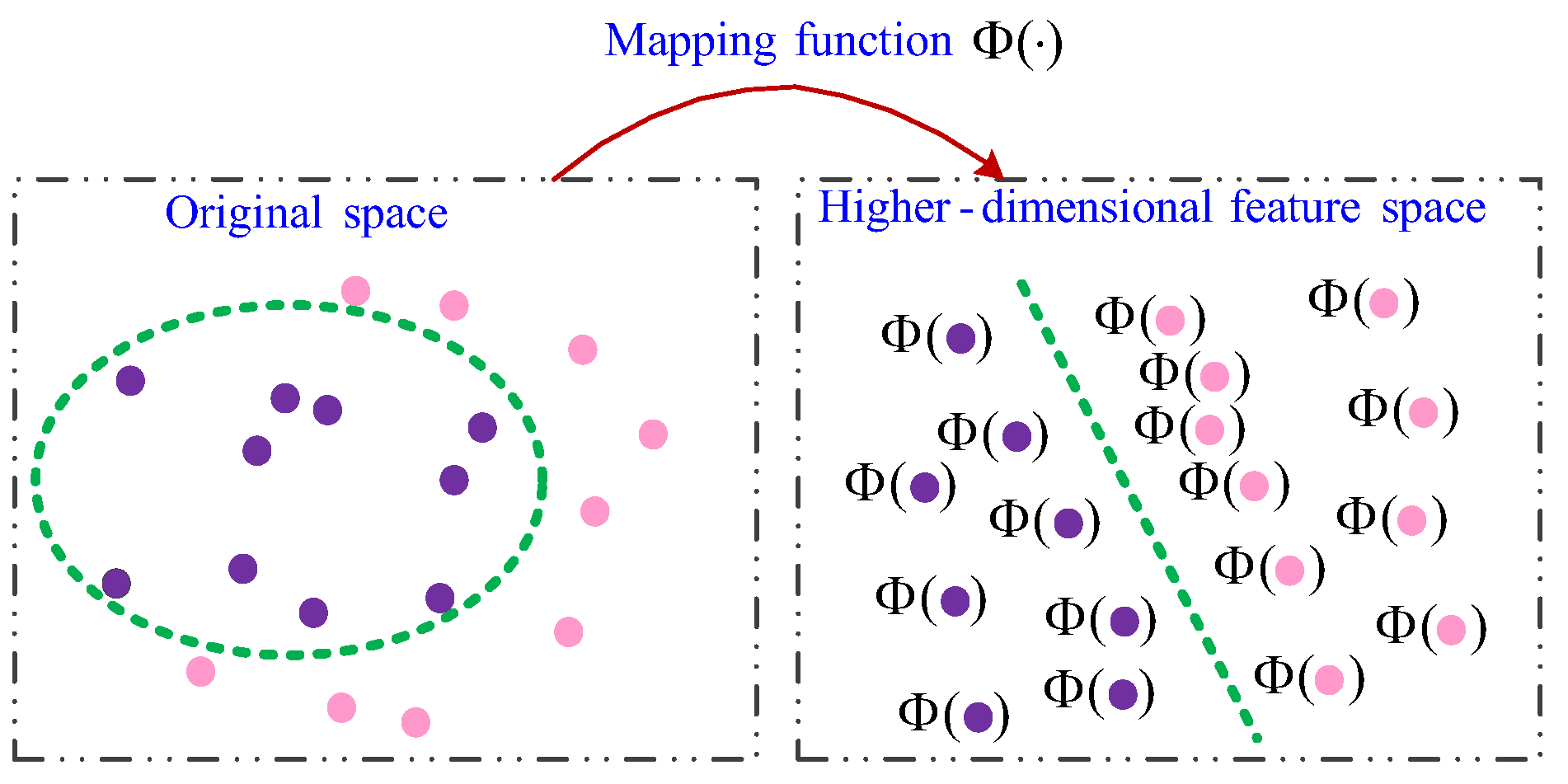
For the nonlinearly separable samples, SVM first maps the data into a higher-dimensional feature space where the points are linearly separable, as shown in Figure 6.

Let $\Phi \left(\mathit{z}\right)$ be the nonlinear mapping function, then (26) in the higher-dimensional feature space is:

$$\begin{array}{l}\min : \frac{1}{2}{\left|\left|\mathit{a}\right|\right|}^2\\ \mathrm{s}.\mathrm{t}.y_i^{\left(t\right)}({\mathit{a}}^{\mathrm{T}}\Phi \left({\mathit{z}}_i^{\left(t\right)}\right)+b)\ge 1 (i=1,2,\cdots ,N_t)\end{array}$$

(27)

Furthermore, SVM can be extended to allow for imperfect separation by penalizing the data falling between $P_1$ and $P_2$. First, we introduce the nonnegative slack variables ${\xi }_i\ge 0$ so that:

$$\begin{array}{l}{\mathit{a}}^{\mathrm{T}}\Phi \left({\mathit{z}}_i^{\left(t\right)}\right)+b\ge +1-{\xi }_i \mathrm{for} y_i^{\left(t\right)}=+1\\ {\mathit{a}}^{\mathrm{T}}\Phi \left({\mathit{z}}_i^{\left(t\right)}\right)+b\le -1+{\xi }_i \mathrm{for} y_i^{\left(t\right)}=-1\end{array}$$

(28)

Then, add a penalizing term to the objective function in (27), and the optimization problem in (27) is now formulated as:

$$\begin{array}{ll}\min :& \frac{1}{2}{\left|\left|\mathit{a}\right|\right|}^2+\eta {\displaystyle {\displaystyle \sum }_{i=1}^{N_t}}{\xi }_i\\ \mathrm{s}.\mathrm{t}. & y_i^{\left(t\right)}({\mathit{a}}^{\mathrm{T}}\Phi \left({\mathit{z}}_i^{\left(t\right)}\right)+b)-1+{\xi }_i\ge 0 (i=1,2,\cdots ,N_t)\\ & {\xi }_i\ge 0, i=1,2,\cdots ,N_t\end{array}$$

(29)

where $\eta$ is the penalty factor.

The Lagrangian function for (29) is:

$$L\left(\mathit{a},b,\mathsf{\xi },\mathit{\alpha },\mathit{\gamma }\right)=\frac{1}{2}{\mathit{a}}^{\mathrm{T}}\mathit{a}+\eta {\displaystyle \sum }_{i=1}^{N_t}{\xi }_i-{\displaystyle \sum }_{i=1}^{N_t}{\alpha }_i[y_i^{(t)}({\mathit{a}}^{\mathrm{T}}\Phi ({\mathit{z}}_i^{\left(t\right)})+b)-1+{\xi }_i]-{\displaystyle \sum }_{i=1}^{N_t}{\gamma }_i{\xi }_i$$

(30)

where ${\left\{{\alpha }_i\right\}}_{i=1}^{N_t}$ and ${\left\{{\gamma }_i\right\}}_{i=1}^{N_t}$ are Lagrange multipliers satisfying ${\alpha }_i\ge 0$ and ${\gamma }_i\ge 0$ for $i=1,2,\cdots ,N_t$.

Then, the optimization problem (29) can be converted into:

$$\underset{\mathit{a},b,\mathsf{\xi }}{\min }\underset{\mathit{\alpha }\ge 0,\mathit{\gamma }\ge 0}{\max }L\left(\mathit{a},b,\mathsf{\xi },\mathit{\alpha },\mathit{\gamma }\right) \mathrm{or} \underset{\mathit{\alpha }\ge 0,\mathit{\gamma }\ge 0}{\max }\underset{\mathit{a},b,\mathsf{\xi }}{\min }L\left(\mathit{a},b,\mathsf{\xi },\mathit{\alpha },\mathit{\gamma }\right)$$

(31)

The KKT conditions corresponding to (31) are as follows:

$$\frac{\partial L\left(\mathit{a},b,\mathsf{\xi },\mathit{\alpha },\mathit{\gamma }\right)}{\partial \mathit{a}}=0\to \mathit{a}={\displaystyle \sum }_{i=1}^{N_t}{\alpha }_i{y}_i^{\left(t\right)}\Phi ({\mathit{z}}_i^{\left(t\right)})$$

(32)

$$\frac{\partial L\left(\mathit{a},b,\mathsf{\xi },\mathit{\alpha },\mathit{\gamma }\right)}{\partial b}=0\to {\displaystyle \sum }_{i=1}^{N_t}{\alpha }_i{y}_i^{\left(t\right)}=0$$

(33)

$$\frac{\partial L\left(\mathit{a},b,\mathsf{\xi },\mathit{\alpha },\mathit{\gamma }\right)}{\partial \mathsf{\xi }}=0\to \eta -{\alpha }_i-{\gamma }_i=0$$

(34)

$${\alpha }_i[y_i^{\left(t\right)}({\mathit{a}}^{\mathrm{T}}\Phi ({\mathit{z}}_i^{\left(t\right)})+b)-1+{\xi }_i]=0$$

(35)

$${\gamma }_i{\xi }_i=0\to \left(P-{\alpha }_i\right){\xi }_i=0$$

(36)

From conditions (35) and (36), it is seen that when $0<{\alpha }_i<P,$ we can get ${\xi }_i=0$ and $y_i^{(t)}({\mathit{a}}^{\mathrm{T}}\Phi ({\mathit{z}}_i^{\left(t\right)})+b)-1=0$, thus $b=1/y_i^{(t)}-{\mathit{a}}^{\mathrm{T}}\Phi ({\mathit{z}}_i^{(t)})$. Combining (32) we get $b=1/y_i^{\left(t\right)}-\Phi ({\mathit{z}}_i^{\left(t\right)})\sum _{j=1}^{N_t}{\alpha }_j{y}_j^{\left(t\right)}\Phi ({\mathit{z}}_j^{\left(t\right)})$.

Taking (32)–(34) into (31), we can obtain:

$$\begin{array}{l}\underset{\mathit{\alpha }\ge 0}{\max }:{\displaystyle {\displaystyle \sum }_{i=1}^{N_t}}{\alpha }_i-\frac{1}{2}{\displaystyle {\displaystyle \sum }_{i,j=1}^{N_t}}{\alpha }_i{\alpha }_j{y}_i^{\left(t\right)}{y}_j^{\left(t\right)}\Phi ({\mathit{z}}_i^{\left(t\right)})\Phi ({\mathit{z}}_j^{\left(t\right)})\\ s.t. {\displaystyle {\displaystyle \sum }_{i=1}^{N_t}}{\alpha }_i{y}_i^{\left(t\right)}=0\\ 0<{\alpha }_i<\eta , i=1,2,\cdots ,N_t\end{array}$$

(37)

Let $k({\mathit{z}}_i^{\left(t\right)},{\mathit{z}}_j^{\left(t\right)})=\Phi ({\mathit{z}}_i^{\left(t\right)})\Phi ({\mathit{z}}_j^{\left(t\right)})$ be the kernel function. We do not need to know the explicit expression of the mapping function $\Phi (\mathit{z})$, as long as the kernel function $k({\mathit{z}}_i^{(t)},{\mathit{z}}_j^{(t)})$ is known.

For an arbitrary untrained point $\mathit{z}$, its label predicted by the trained SVM is:

$$s\left(\mathit{z}\right)=s\left[{\displaystyle \sum }_{j=1}^{N_{\ast }}{\alpha }_j^{\ast }{y}_j^{\ast }k(\mathit{z},{\mathit{z}}_j^{\ast })+b\right]$$

(38)

where $s\left(\mathit{z}\right)$ is the symbolic function, ${\mathit{z}}_j^{\ast }$ for $j=1,2,\cdots ,N_{\ast }$ are $N_{\ast }$ support vectors, and $y_j^{\ast }$ is the sign of ${\mathit{z}}_j^{\ast }$. ${\alpha }_j^{\ast }$ represents the Lagrange multiplier corresponding to support vector ${\mathit{z}}_j^{\ast }$.

Remark 1.

Only those samples that lie closest to the decision boundary $P$satisfy ${\alpha }_i>0$, and these samples are referred to as the support vectors (just as the “*” points in Figure 5b). For the non-support vectors, their corresponding Lagrange multipliers equal zero.

Remark 2.

Parameter b can be solved by any support vector, but for accuracy, the estimate of b corresponding to each support vector is calculated, and their mean value is taken as the final estimate of b.

Remark 3.

The soft penalty $\eta$permits the misclassification. Increasing $\eta$generates a stricter classification. If we reduce $\eta$towards 0, it makes misclassification less important; if we increase $\eta$to infinity, it means no misclassification is allowed.

Till now, we have expounded the basic idea of SVM. Hereinafter, the procedure of SVM for constructing the alternative models ${\widehat{I}}_F\left(\mathit{z}\right)$ and ${\widehat{I}}_{\lambda }\left(\mathit{z}\right)$ are demonstrated, as shown in Algorithms 2 and 3, respectively.

Algorithm 2 SVM for constructing the alternative model ${\widehat{I}}_F\left(\mathit{z}\right)$
1.	Let ${\mathit{S}}_f$ be the set of feasible individuals, and ${\mathit{S}}_{inf}$ be the collection of infeasible individuals.
2.	The labels of individuals of ${\mathit{S}}_f$ are “+1,” while the labels of individuals of ${\mathit{S}}_{inf}$ are “−1.”
3.	Let $\mathit{S}={\mathit{S}}_f{\displaystyle \bigcup }{\mathit{S}}_{inf}$, and ${\mathit{L}}_{\mathit{S}}$ is the set consisting of the labels of individuals in $\mathit{S}$.
4.	Construct the alternative model ${\widehat{I}}_F\left(\mathit{z}\right)$ by using data set $\left(\mathit{S},{\mathit{L}}_{\mathit{S}}\right)$.

Algorithm 3 SVM for constructing the alternative model ${\widehat{I}}_{\lambda }\left(\mathit{z}\right)$
1.	Let ${\mathit{S}}_f=\{{\mathit{z}}_1^{\left(f\right)},{\mathit{z}}_2^{\left(f\right)},\cdots ,{\mathit{z}}_{N_f}^{\left(f\right)}\}$ be the set of feasible individuals, where $N_f$ is the size of ${\mathit{S}}_f$.
2.	Calculate objective function values $\{H({\mathit{z}}_1^{\left(f\right)}),H({\mathit{z}}_2^{\left(f\right)}),\cdots ,H({\mathit{z}}_{N_f}^{\left(f\right)})\}$.
3.	Arrange these objective function values in descending order, i.e., $H({\mathit{z}}_{\left[1\right]}^{\left(f\right)})>H({\mathit{z}}_{\left[2\right]}^{\left(f\right)})>\cdots >H({\mathit{z}}_{\left[N_f\right]}^{\left(f\right)})$.
4.	Set a probability $p_0\in \left(0,1\right)$.
5.	Let $\lambda =H({\mathit{z}}_{\left[p_0{N}_f\right]}^{\left(f\right)})$ be the threshold that divides superior/inferior individuals.
6.	Divide ${\mathit{S}}_f$ into two sets: a set ${\mathit{S}}_{-}$ with individuals whose objective function values are larger than λ, and the other set ${\mathit{S}}_{+}$ of individuals whose objective function values are smaller than λ.
7.	The labels of individuals in ${\mathit{S}}_{-}$ are “−1,” and the labels of individuals in ${\mathit{S}}_{+}$ are “+1.”
8.	Let ${\mathit{L}}_{{\mathit{S}}_f}$ be the set of labels of ${\mathit{S}}_f$.
9.	Establish the alternative model ${\widehat{I}}_{\lambda }\left(\mathit{z}\right)$ by using training sample set $\left({\mathit{S}}_f,{\mathit{L}}_{{\mathit{S}}_f}\right)$.

It should be noted that in Algorithms 2 and 3, we use “−1” and “+1” to represent the symbols of the two types of samples, but in fact, when we code our algorithm, we use “0” instead of “−1” to label the unwanted point, or we can use transformations:

$${\widehat{I}}_F\left(\mathit{z}\right)=\{\begin{array}{c}1 \mathrm{if} \mathrm{the} \mathrm{label} \mathrm{of} \mathit{z} \mathrm{is}+1\\ 0 \mathrm{if} \mathrm{the} \mathrm{label} \mathrm{of} \mathit{z} \mathrm{is}-1\end{array}$$

and

$${\widehat{I}}_{\lambda }\left(\mathit{z}\right)=\{\begin{array}{c}1 \mathrm{if} \mathrm{the} \mathrm{label} \mathrm{of} \mathit{z} \mathrm{is}+1\\ 0 \mathrm{if} \mathrm{the} \mathrm{label} \mathrm{of} \mathit{z} \mathrm{is}-1\end{array}$$

to make ${\widehat{I}}_F\left(\mathit{z}\right)$ and ${\widehat{I}}_{\lambda }\left(\mathit{z}\right)$ can be utilized to construct the quasi-optimal IS PDF. This is also applicable for Algorithm 4.

3.3. General Whole Algorithm of the Proposed Solution Procedure

In this section, the concrete solution procedure of the proposed approach for solving the optimization problem is demonstrated. The general whole algorithm of the proposed approach is Algorithm 4, and the corresponding flowchart is depicted in Figure 7.

Algorithm 4 The general process of the proposed optimization approach
1.	Let ${\mathit{z}}_l^{\ast }$ be the initial solution of decision variables, and $l=0$.
2.	Set a value to $p_0$.
3.	Produce the first-generation population ${\mathit{S}}^{\left(l\right)}=\{{\mathit{z}}_1^{\left(l\right)},{\mathit{z}}_2^{\left(l\right)},\cdots ,{\mathit{z}}_{N_l}^{\left(l\right)}\}$.
4.	Let $\mathit{S}={\mathit{S}}^{\left(l\right)}$.
	For $l=0:1:Ite{r}_{m\mathit{a}x}$, do:
5.	Evaluate whether the individuals in ${\mathit{S}}^{\left(l\right)}$ satisfy the given constraints.
6.	Sift out the feasible individuals ${\mathit{S}}_f=\{{\mathit{z}}_1^{\left(f\right)},{\mathit{z}}_2^{\left(f\right)},\cdots ,{\mathit{z}}_{N_f}^{\left(f\right)}\}$ and infeasible individuals ${\mathit{S}}_{inf}={\mathit{S}}^{\left(l\right)}\backslash {\mathit{S}}_f$.
7.	Update the current optimal solution as ${\mathit{z}}_{l+1}^{\ast }={\mathrm{argmin}}_{\mathit{z}\in {\mathit{S}}_f}H\left(\mathit{z}\right)$.
8.	Calculate $E_r=|H({\mathit{z}}_{l+1}^{\ast })-H({\mathit{z}}_l^{\ast })|/|H({\mathit{z}}_{l+1}^{\ast })|$.
	If $E_r\le \epsilon$ ($\epsilon \to 0^{+}$ is a small real number)
	Break
	End if
9.	Construct/update the classifier ${\widehat{I}}_F\left(\mathit{z}\right)$ dividing the feasible/infeasible domains via SVM.
	9.1. Label “+1” to feasible individuals and “−1” to infeasible individuals, for individuals in $\mathit{S}$.
	9.2. Let ${\mathit{L}}_{\mathit{S}}$ be the set of labels of individuals in $\mathit{S}$.
	9.3. Construct/update ${\widehat{I}}_F\left(\mathit{z}\right)$ by using $\left(\mathit{S},{\mathit{L}}_{\mathit{S}}\right)$.
10.	Construct the classifier ${\widehat{I}}_{\lambda }\left(\mathit{z}\right)$ via SVM.
	10.1. Rank the objective function values of ${\mathit{S}}_f$ in descending order, i.e., $H({\mathit{x}}_{\left[1\right]}^{\left(f\right)})>H({\mathit{x}}_{\left[2\right]}^{\left(f\right)})>\cdots >H({\mathit{x}}_{\left[N_f\right]}^{\left(f\right)})$.
	10.2. Let the $p_0$th objective function value be the threshold, i.e., $\lambda =H({\mathit{x}}_{\left[p_0{N}_f\right]}^{\left(f\right)})$.
	10.3. Divide ${\mathit{S}}_f$ as superior individuals ${\mathit{S}}_{+}$ with objective function values smaller than $\lambda$, and inferior individuals ${\mathit{S}}_{-}$ with objective function values larger than $\lambda$.
	10.4. Label “+1” to individuals in ${\mathit{S}}_{+}$ and “−1” to individuals in ${\mathit{S}}_{-}$.
	10.5. Construct the classifier ${\widehat{I}}_{\lambda }\left(\mathit{z}\right)$ by using $\left({\mathit{S}}_f,{\mathit{L}}_{{\mathit{S}}_f}\right)$.
11.	Produce the next-generation population ${\mathit{S}}^{\left(l+1\right)}$.
	11.1. Construct the quasi-optimal IS PDF ${\widehat{g}}_{opt}\left(\mathit{z}\right)={\widehat{I}}_F\left(\mathit{z}\right){\widehat{I}}_{\lambda }\left(\mathit{z}\right)f\left(\mathit{z}\right)/\int {\widehat{I}}_F\left(\mathit{z}\right){\widehat{I}}_{\lambda }\left(\mathit{z}\right)f\left(\mathit{z}\right)d\mathit{z}$.
	11.2. Generate the next-generation population ${\mathit{S}}^{\left(l+1\right)}=\{{\mathit{z}}_1^{\left(l+1\right)},{\mathit{z}}_2^{\left(l+1\right)},\cdots ,{\mathit{z}}_{N_{l+1}}^{\left(l+1\right)}\}$ in terms of ${\widehat{g}}_{opt}\left(\mathit{z}\right)$.
12.	Let $\mathit{S}=\mathit{S}{\displaystyle \bigcup }{\mathit{S}}^{\left(l+1\right)}$.
	End for
13.	Output the optimal decision scheme ${\mathit{z}}_{opt}^{\ast }={\mathit{z}}_{l+1}^{\ast }$.

Some details of Algorithm 4 are as follows.

(1)

The initial solution ${\mathit{z}}_l^{\ast } \left(l=0\right)$ can be a feasible solution or an arbitrary point in the design domain. It does not affect the quality of the whole algorithm, since it is just used as an extra stopping condition. In addition, the maximum number of iterations could be conveniently set to $Ite{r}_{m\mathit{a}x}=100$.

(2)

The preset probability $p_0\in \left(0,1\right)$ divides feasible individuals into two groups: the group whose objective function value is smaller than $\lambda =H({\mathit{x}}_{\left[p_0{N}_f\right]}^{\left(f\right)})$, and the other group, whose objective function value is larger than $\lambda$. From the perspective of fitness, the former group of samples are excellent individuals with “high” fitness and should be retained to produce offspring. The latter group of samples do not adapt to the current environment and are inferior individuals that will be discarded. Of course, the choice of $p_0$ directly affects the convergence speed of the algorithm and whether the optimal solution can be found.

(3)

In step 9, we construct the initial SVM model ${\widehat{I}}_F\left(\mathit{z}\right)$ by using the initial information of the feasible/infeasible domains. Then, the SVM model ${\widehat{I}}_F\left(\mathit{z}\right)$ will be updated by the expanded data set (see step 12). This adequately excavates the information of the design domain, and thus we can construct a more precise asymptotical boundary to separate the feasible domain from the infeasible domain.

(4)

The quasi-optimal IS PDF ${\widehat{g}}_{opt}\left(\mathit{z}\right)$ is established by using the constructed SVM models ${\widehat{I}}_F\left(\mathit{z}\right)$ and ${\widehat{I}}_{\lambda }\left(\mathit{z}\right)$. Since the denominator $\int {\widehat{I}}_F\left(\mathit{z}\right){\widehat{I}}_{\lambda }\left(\mathit{z}\right)f\left(\mathit{z}\right)d\mathit{z}$ is a constant that does not affect the probability density, we can only utilize the numerator ${\widehat{I}}_F\left(\mathit{z}\right){\widehat{I}}_{\lambda }\left(\mathit{z}\right)f\left(\mathit{z}\right)$ to produce the offspring. Furthermore, since we only know the lower and upper bounds of decision variables z, it is convenient to regard that the prior distribution of $\mathit{z}$ is uniform. That is, $f\left(\mathit{z}\right)$ is a constant, so we can use ${\widehat{I}}_F\left(\mathit{z}\right){\widehat{I}}_{\lambda }\left(\mathit{z}\right)$ to produce new individuals. The modified Metropolis–Hastings sampler is applied to generate the quasi-optimal new individuals, and the thinning procedure is used to ensure these individuals are independent [31].

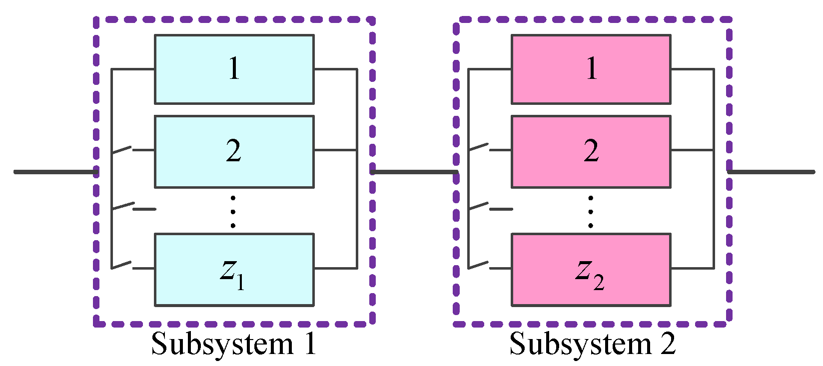
Example 2.

Consider the case study in Example 1. Here, we set$k=1$and$n=2$, then the Lin/Con/$k$/$n$:F system is reduced to a series system with two subsystems, as shown in Figure 8. For a subsystem$j\in \left\{1,2\right\}$, it involves an active-standby component and${\mathit{z}}_j-1$cold-standby redundant components.

Meanwhile, the system reliability is reduced to:

$$R_s\left(t;\mathit{z}\right)={\displaystyle \prod }_{j=1}^2\left(r_j\left(t\right)+{({\rho }_j)}^{{\mathit{z}}_j-1}{\displaystyle \sum }_{s=1}^{{\mathit{z}}_j-1}\frac{{\left({\beta }_{j}t\right)}^s\exp \left(-{\beta }_{j}t\right)}{s!}\right)$$

(39)

where the redundancy level $\mathit{z}=\left\{{\mathit{z}}_1,{\mathit{z}}_2\right\}$ is the decision vector. Suppose that the component reliabilities for subsystem 1 and subsystem 2 are 0.93 and 0.92, respectively. The reliability of each switch is 0.9998. In addition, ${\beta }_1=5\times {10}^{-5}$, ${\beta }_2=4\times {10}^{-5}$, and $t=1400 \left(\mathrm{h}\right)$.

The mathematical model of the optimization problem of this example under budget constraint is:

$$\begin{array}{l}\underset{\mathit{z}}{\max :}\left(39\right)\\ \mathrm{s}.\mathrm{t}. G\left(\mathit{z}\right)={\displaystyle {\displaystyle \sum }_{i=1}^2}({\mathit{z}}_i^2+{\mathit{z}}_i|\cos \left(\pi r_i\right)|)-C\le 0\\ 2\le {\mathit{z}}_i\le 5, {\mathit{z}}_i\in {\mathbb{N}}_{+} \left(i=1,2\right)\end{array}$$

where $C=27$ is the budget constraint.

For comparison, we first utilize GA to explore the optimal decision scheme of this optimization problem. The obtained optimal decision scheme is ${\mathit{z}}_{opt}^{\ast }=\left\{3,3\right\}$, and the corresponding system reliability is $R_s\left(\mathit{z}\right)=0.971999$. The value of the constraint function is $\mathrm{G}\left(\mathit{z}\right)=-3.1665$, which indicates that the constraint is satisfied. Then, we implement the proposed approach to address this optimization problem. The initial solution is chosen as ${\mathit{z}}_0^{\ast }=\left\{2,2\right\}$. Through two iterations, the optimal solution obtained by the proposed approach is also ${\mathit{z}}_{opt}^{\ast }=\left\{3,3\right\}$. 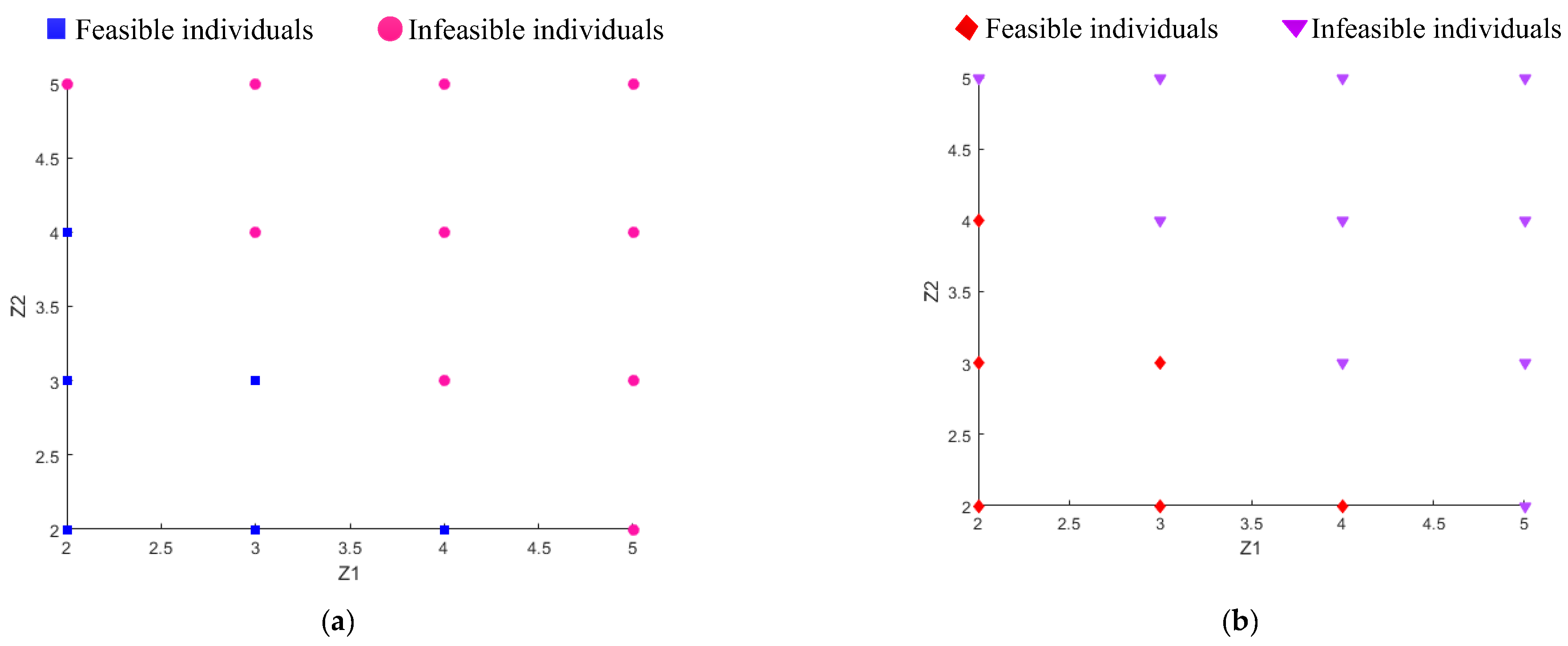This is consistent with that obtained by GA. To showcase the quality of the alternative model constructed by SVM, the feasible/infeasible candidates distinguished by SVM and the actual constraint function are shown in Figure 9a and Figure 9b, respectively. It is seen that the constructed alternative model is sufficiently accurate to separate feasible individuals from infeasible individuals.

3.4. Discussion

(1)

The quasi-optimal IS PDF embedded in the proposed approach facilitates producing high-quality offspring. Different from other reproduction algorithms, it is a deterministic rather than a stochastic strategy. Most importantly, it does not need to determine a series of parameters, which is critical to the robustness of the algorithm. In addition, this distribution does not give a larger weight to a certain individual, but gives weight according to the contribution of each feasible individual. This ensures the diversity of offspring, and avoids the degeneration of offspring or the emergence of super individuals (local optima).

(2)

The classifiers constructed by SVM avoid the repeat invocation of objective and constraint functions during the process of producing offspring. For complex systems, this is of monumental significance in mitigating the computational burden, but we have to point out that if the actual boundary is highly nonlinear, the alternative boundary constructed by SVM may deviate from the actual one. In addition, standardizing the training data will be helpful to improve the quality of the constructed classifier.

(3)

There is no limit on the objective function or constraint function. We just utilize the objective function to measure the fitness of feasible individuals, and use the constraint functions to evaluate whether an individual is a feasible one. Therefore, the proposed approach is suitable for a wide range of problems.

(4)

The proposed algorithm involves few parameters. It usually only needs to determine the parameter $p_0$ for dividing superior/inferior individuals and the population size $N$ of each generation. Hence, the proposed algorithm is easy to implement.

(5)

If $\mathit{z}$ is a set of integer design variables or mixed integer-real design variables, we first treat the integer decision variables as real variables. The population of real decision variables are generated in the design domain. Then, we round the new population to produce new integer individuals.

4. Numerical Results

Consider the Lin/Con/$k$/$n$:F system shown in Figure 2. Here, we assume that the reliability of component in each subsystem is unknown and should be designed. In addition, the corresponding redundancy level is also a decision variable. Hence, the decision vector is denoted $\mathit{z}=\left\{{\mathit{z}}_1,{\mathit{z}}_2,\cdots ,{\mathit{z}}_n,{\mathit{z}}_{n+1},\cdots ,{\mathit{z}}_{2n}\right\}$, where ${\mathit{z}}_i\in ℝ$ for $i=1,2,\cdots ,n$ denotes the reliability choice of each subsystem, while ${\mathit{z}}_i\in {\mathbb{N}}_{+}$ for $i=n+1,n+2,\cdots ,2n$ represents the redundancy level of each subsystem. The system-level constraints are budget constraint and volume constraint. The mathematical model of this optimization problem is formulated as:

$$\begin{array}{ll}\underset{\mathit{z}}{\max :}& R_s\left(t;k,n\right)={\displaystyle {\displaystyle \sum }_{i=n-k+1}^n}{R}_i\left(t\right)R_s\left(t;k,i-1\right){\displaystyle {\displaystyle \prod }_{j=i+1}^n}\left(1-R_j\left(t\right)\right)\\ \mathrm{s}.\mathrm{t}. & G_1\left(\mathit{z}\right)={\displaystyle {\displaystyle \sum }_{i=1}^n}(c_i{\mathit{z}}_{i+n}^2+{\mathit{z}}_{i+n}|\cos \left(\pi {\mathit{z}}_i\right)|)-C\le 0\\ & G_2\left(\mathit{z}\right)={\displaystyle {\displaystyle \sum }_{i=1}^n}{v}_i{\mathit{z}}_{i+n}-V\le 0\\ & z_i^L\le z_i\le z_i^U \left(z_i\in ℝ, i=1,2,\cdots ,n\right)\\ & z_i^L\le z_i\le z_i^U \left(z_i\in {\mathbb{N}}_{+}, i=n+1,n+2,\cdots ,2n\right)\end{array}$$

where

$$R_i\left(t\right)=z_i\left(t\right)+{({\rho }_i)}^{z_{i+n}-1}{\displaystyle \sum }_{s=1}^{z_{i+n}-1}\frac{{\left({\beta }_{i}t\right)}^s\exp \left(-{\beta }_{i}t\right)}{s!}$$

The parameters $C$, $V$, $\mathit{c}=\left\{c_i,i=1,2,\cdots ,n\right\}$ and $\mathit{\nu }=\left\{v_i,i=1,2,\cdots ,n\right\}$ involved in constraint functions are set according to the problem at hand. In the following, we present the performance of the proposed approach by investigating different cases.

4.1. Lin/Con/2/10:F System

For this case, $k=2$ and $n=10$. Thus, this is a 20-dimensional optimization problem. For simplicity, we set $C=80$, $V=50$, $\mathit{c}=0.8\times {\mathbf{1}}_{1\times n}$, and $\mathit{\nu }=1.5\times {\mathbf{1}}_{1\times n}$. The switch’s reliability of each subsystem is 0.9999, and the parameter of the exponential time-to-failure model of each subsystem is $5\times {10}^{-5}$. The time interval we investigate is [0, 1000]. The variation domain of decision variables is $0.9\le {\mathit{z}}_i\le 0.94 \left(i=1,2,\cdots ,n\right)$ and ${\mathit{z}}_i\in \left\{2,3,4\right\} \left(i=n+1,n+2,\cdots ,2n\right)$.

Then, we implement GA and the proposed approach to search for the optimal solution of this optimization problem. The system reliability obtained by these two approaches as well as the corresponding consumed CPU time are listed in Figure 10. These results are calculated under different choices of $p_0$ for the proposed approach, crossover fractions $c_f$ for GA, and population sizes $N$. From the listed results we can draw the following conclusions.

(1)

Under the same population size $N$, the system reliability corresponding to the optimal solution obtained by the proposed algorithm tends to be higher than that obtained by GA, because the system reliability curve obtained by the proposed approach is almost above that obtained by GA, except in several special cases. Meanwhile, the CPU time consumed by the proposed algorithm is longer than that consumed by GA, that is, the efficiency of the proposed algorithm is slightly lower than that of GA.

(2)

For this example, in general, the selection of $p_0$ has little impact on the system reliability obtained by the proposed algorithm, except for the case under $N=100$ (there is a sudden drop when $p_0=0.9$). In contrast, the choice of $p_0$ has an obvious impact on the efficiency of the proposed algorithm, because the curve related to the CPU time fluctuates greatly.

(3)

The choice of crossover fraction $c_f$ largely influences the accuracy of GA, because it is obvious that the system reliability curve obtained by GA fluctuates greatly with $c_f$. In addition, the crossover fraction $c_f$ does not seem to have much effect on the efficiency of GA.

(4)

As the population size $N$ increases, the CPU time required for the proposed algorithm or GA increases gradually. Of course, this is a predictable result.

Figure 10. Results of the Lin/Con/2/10:F system. (a) Results under N = 100; (b) Results under N = 300; (c) Results under N = 700; (d) Results under N = 900; (e) Results under N = 1000; (f) Optimal system reliability under different N.

Figure 10. Results of the Lin/Con/2/10:F system. (a) Results under N = 100; (b) Results under N = 300; (c) Results under N = 700; (d) Results under N = 900; (e) Results under N = 1000; (f) Optimal system reliability under different N.

Figure 10f demonstrates the best results obtained by GA and the proposed approach under different population sizes. We can also observe that the population size $N$ almost has no effect on the final solution obtained by the proposed approach, but has large effect on the solution obtained by GA. The best optimal solutions obtained by GA and the proposed approach are listed in

Table 1. Optimal solutions of the Lin/Con/2/10:F system.

	GA	Proposed
$z_1$	0.939999982082880	0.939999968151024
$z_2$	0.939999998470598	0.939999966167825
$z_3$	0.939999986747398	0.939999938687086
$z_4$	0.939999897636930	0.939999959575710
$z_5$	0.939999907059162	0.939999979766451
$z_6$	0.939999654750784	0.939999976480183
$z_7$	0.939999989639616	0.939999994470781
$z_8$	0.939999723723163	0.939999969973595
$z_9$	0.939999955439849	0.939999976556797
$z_{10}$	0.939999968667557	0.939999979670160
$z_{11}–z_{20}$	2, 3, 3, 2, 3, 2, 3, 2, 3, 2	2, 3, 2, 3, 2, 3, 2, 3, 3, 2
$R_s$	0.998765905257641	0.998765919621590
$G_1$	−3.442819929273583	−3.442819162838759
$G_2$	−12.5	−12.5
Time (s)	2.295923	145.862364

.

From Table 1, we can see that the final system reliability obtained by the proposed approach is larger than that obtained by GA. Moreover, the final decision schemes obtained by these two approaches all satisfy the given constraints, because the values of these two constraint functions are all smaller than 0. However, the proposed approach needs a longer time to explore the optimal solution. That is, the proposed approach tends to obtain a more reliable system, but sacrifices CPU time. For this example, the parameter settings of the proposed approach almost have no effect on the final system reliability, but somewhat affect the computational efficiency.

4.2. Lin/Con/3/50:F System

In this section, we consider a Lin/Con/3/50:F system, i.e., $n=50$ and $k=3$. This system fails if three consecutive subsystems fail. The design task of this system is to find the optimal reliability choice for each subsystem and its corresponding redundancy level; thus, it is a 100-dimension problem. As for the parameters involved in constraint functions, we set $C=370$, $V=170$, $\mathit{c}=0.5\times {\mathbf{1}}_{1\times n}$ and $\mathit{\nu }=1.2\times {\mathbf{1}}_{1\times n}$. The parameters related to the exponential time-to-failure assumption are ${\mathsf{\beta }}_i=1\times {10}^{-5}$ for $i=1,2,\cdots ,n$. The reliability of the switch of each subsystem is 0.9998. The time interval we investigate is [0, 1200]. The decision variables satisfy $0.9\le {\mathit{z}}_i\le 0.94 \left(i=1,2,\cdots ,n\right)$ and ${\mathit{z}}_i\in \left\{2,3,4\right\} \left(i=n+1,n+2,\cdots ,2n\right)$.

Similarly, we first investigate the performance of the proposed approach under different parameter settings. Specifically, we study the performance of the proposed approach varying with the population size $N$ or choice of $p_0$. Furthermore, for comparison, we also list the results obtained by GA under different parameter settings. The comparison results are depicted in Figure 11.

From Figure 11, we can observe that from the perspective of the final solution, it seems that the proposed approach is likely to procure more reliable systems compared with GA, because under different scenarios, the system reliability curve obtained by the proposed approach is always lying above that obtained by GA. As for the computational effort, the proposed approach needs longer time to explore the design domain than GA.

Under the assumptions of this example, we also can conclude that the choice of $p_0$ has little effect on the final decision scheme, because under a fixed population size $N$, the system reliability curve varies slightly. In contrast, the computational cost curve waves largely with $p_0$. As for the population size $N$, from Figure 11f we can see directly that $N$ has relatively large influence on the final system reliability, meanwhile, it also severely affects the computational efficiency.

The best optimal solutions obtained by GA and the proposed approach are listed in

Table 2. Optimal solutions of the Lin/Con/3/50:F system.

	GA	Proposed
$z_1$	0.939999997323903	0.939999101574871
$z_2$	0.939999986959498	0.939999708813599
$z_3$	0.939999999440908	0.939999664472164
$z_4$	0.939999999794802	0.939999666796851
$z_5$	0.939999999935371	0.939999168877791
$z_6$	0.939999998110852	0.939999679837133
$z_7$	0.939999993493591	0.939999088778805
$z_8$	0.939999994570576	0.939999461975156
$z_9$	0.939999872727478	0.939999520118700
$z_{10}$	0.939999999119440	0.939999013016654
$z_{11}$	0.939999985392297	0.939999943244986
$z_{12}$	0.939999999906751	0.939999026955801
$z_{13}$	0.939999993129890	0.939999886135686
$z_{14}$	0.939999944037610	0.939999872726818
$z_{15}$	0.939999993059754	0.939999699713407
$z_{16}$	0.939999999543360	0.939999797929416
$z_{17}$	0.939999998853268	0.939999516500447
$z_{18}$	0.939999694489169	0.939999931861274
$z_{19}$	0.939999999589299	0.939999618328248
$z_{20}$	0.939999998801516	0.939999539553962
$z_{21}$	0.939999995020908	0.939999177884446
$z_{22}$	0.939999997033384	0.939999978753488
$z_{23}$	0.939999999269234	0.939999676568527
$z_{24}$	0.939999848696102	0.939999307955568
$z_{25}$	0.939999997244683	0.939999297303247
$z_{26}$	0.939999975228799	0.939999655372835
$z_{27}$	0.939999999351067	0.939999424186198
$z_{28}$	0.939999999444971	0.939999117361033
$z_{29}$	0.939999998613960	0.939999680655764
$z_{30}$	0.939999990057712	0.939999363122079
$z_{31}$	0.939999993030546	0.939999565479744
$z_{32}$	0.939999981123084	0.939999657580338
$z_{33}$	0.939999997448862	0.939999403008793
$z_{34}$	0.939999475165336	0.939999987364082
$z_{35}$	0.939999992356452	0.939999186977101
$z_{36}$	0.939999999906650	0.939999300609624
$z_{37}$	0.939999997249567	0.939999526578020
$z_{38}$	0.939999940356929	0.939999335505310
$z_{39}$	0.939999989207330	0.939999503094603
$z_{40}$	0.939999999091310	0.939999221430349
$z_{41}$	0.939999944483187	0.939999872848627
$z_{42}$	0.939999998521296	0.939999295777140
$z_{43}$	0.939999984415788	0.939999744556439
$z_{44}$	0.939999991112152	0.939999833642483
$z_{45}$	0.939999999622116	0.939999662645608
$z_{46}$	0.939999994551369	0.939999846922115
$z_{47}$	0.939999986649583	0.939999635815842
$z_{48}$	0.939999994150871	0.939999366831244
$z_{49}$	0.939999997928706	0.939999355264495
$z_{50}$	0.939999993095978	0.939999069146052
$z_{51}–z_{100}$	2, 2, 4, 3, 4, 3, 2, 2, 4, 3, 2, 2, 4, 4, 4, 2, 2, 2, 2, 2, 2, 2, 4, 2, 3, 2, 4, 3, 2, 2, 4, 3, 3, 2, 3, 2, 4, 4, 2, 2, 4, 4, 2, 2, 4, 2, 2, 2, 2, 2	3, 4, 3, 3, 3, 2, 3, 3, 2, 2, 2, 3, 3, 2, 3, 3, 3, 2, 3, 2, 3, 3, 3, 3, 3, 3, 3, 2, 3, 4, 3, 3, 2, 3, 3, 3, 3, 3, 2, 3, 3, 3, 3, 3, 3, 2, 3, 4, 2, 3
$R_s$	0.994916477883922	0.994922886980181
$G_1$	−32.408936074006476	−25.997537921650007
$G_2$	−6.799999999999926	−0.800000000000097
Time (s)	22.244123	399.361658

for further comparison. It is seen that the maximum system reliabilities obtained by GA and the proposed approach are 0.994916477883922 and 0.994922886980181, respectively. This indicates that the proposed approach tends to procure more reliable systems compared with GA, but this is achieved by sacrificing CPU time.

4.3. Application Results

Consider the electrical power network system shown in Figure 12a. This system contains transformer substations and electric wires. The electricity starts from the supplier city, and then will be delivered to the target city through electrical wires and transformer substations. Here, we suppose that the wires are very reliable (with reliability approach to 1) and the system reliability only depends on the reliability of the transformer substation shown in Figure 12b. Following [26], the reliability of this network system is as follows:

$$R_s={\displaystyle \sum }_{i=1}^n{\mathit{a}}_i^{\left(1\right)}{r}_i+{\displaystyle \sum }_{i<j}^n{\mathit{a}}_{i,j}^{\left(2\right)}{r}_i{r}_j+{\displaystyle \sum }_{i<j<k}^n{\mathit{a}}_{i,j,k}^{\left(3\right)}{r}_i{r}_j{r}_k+\cdots +{\mathit{a}}_{1,2,\cdots ,n}^{\left(n\right)}{r}_1{r}_2\cdots r_n$$

(40)

where $r_i$ $\left(i=1,2,\cdots ,n\right)$ is the reliability of transformer substation $i$. ${\mathit{a}}_i^{\left(1\right)}$ $\left(i=1,2,\cdots ,n\right)$ is the nonnegative real coefficient for single-variable term, and $\{{\mathit{a}}_{i,j}^{\left(2\right)},{\mathit{a}}_{i,j,k}^{\left(3\right)},\cdots ,{\mathit{a}}_{1,2,\cdots ,n}^{\left(n\right)}\}$ are nonnegative real coefficients for cross-product terms.

The transformer substation is a 25-bar space truss structure whose material mass density is 0.1. The three coordinates of each node and the member grouping information are listed in

Table 3. Nodal coordinates of the truss structure.

Node	X	Y	Z
1	−37.5	0.0	200
2	37.5	0.0	200
3	−37.5	37.5	100
4	37.5	37.5	100
5	37.5	−37.5	100
6	−37.5	−37.5	100
7	−100	100	0.0
8	100	100	0.0
9	100	−100	0.0
10	−100	−100	0.0

and

Table 4. Group membership for the truss structure.

Group	Members
I	1
II	2, 3, 4, 5
III	6, 7, 8, 9
IV	10, 11, 12, 13
V	14, 15, 16, 17, 18, 19, 20, 21
VI	22, 23, 24, 25

, respectively. The cross-sectional area and Young’s modulus of the bar at each group are denoted $A_{\mathrm{I}}–A_{\mathrm{VI}}$ and $E_{\mathrm{I}}–E_{\mathrm{VI}}$, respectively. Four nodal forces $p_{1\mathrm{Y}}=p_{1\mathrm{Z}}=p_{2\mathrm{Y}}=p_{2\mathrm{Z}}=-{10}^4\left(\mathrm{N}\right)$ are applied at node 1 and node 2, while the forces on node 3 and node 6 are $p_{3\mathrm{X}}$ and $p_{6\mathrm{X}}$ with random values. $\left\{A_{\mathrm{I}}–A_{\mathrm{VI}},E_{\mathrm{I}}–E_{\mathrm{VI}},p_{3\mathrm{X}},p_{6\mathrm{X}}\right\}$ are the input variables following normal distribution, and the distribution parameters are listed in

Table 5. Input variables for the truss structure.

No.	Variable	Mean	Variation Coefficient
1	$A_{\mathrm{I}}$	0.5	0.05
2	$A_{\mathrm{II}}$	0.5	0.05
3	$A_{\mathrm{III}}$	2	0.05
4	$A_{\mathrm{IV}}$	0.4	0.05
5	$A_{\mathrm{V}}$	0.5	0.05
6	$A_{\mathrm{VI}}$	2	0.05
7–11	$E_{\mathrm{I}}–E_{\mathrm{V}}$	${10}^7$	0.02
12	$E_{\mathrm{VI}}$	${10}^7$	0.15
13	$p_{3\mathrm{X}}$	$5\times {10}^2$	0.1
14	$p_{6\mathrm{X}}$	$5\times {10}^2$	0.1

. The transformer substation fails if its maximum displacement exceeds 0.80 (m). Here, the displacement is an implicit function related to random inputs, which is obtained by the finite element model (FEM). The FEM analysis result is demonstrated in Figure 13.

To improve the system reliability, we can add redundant bars to the transformer substation and construct the optimization model as follows:

$$\begin{array}{l}\underset{\mathit{z}}{\max :}\left(40\right)\\ \mathrm{s}.\mathrm{t}. G\left(\mathit{z}\right)={\displaystyle {\displaystyle \sum }_{i=1}^6}{\mathit{z}}_i^2-C\le 0\\ 1\le {\mathit{z}}_i\le 5, {\mathit{z}}_i\in {\mathbb{N}}_{+} \left(i=1,2, \cdots ,6\right)\end{array}$$

where $G\left(\mathit{z}\right)$ is the cost constraint with threshold $C=33$. The design variable is the redundancy of each group of bars. Suppose that all the transformer substations are the same, the objective of this problem is equivalent to maximizing the reliability of the transformer substation.

We implement the proposed approach and GA to mine the optimal decision scheme of this system, and the obtained results are listed in

Table 6. Optimal solutions for the application case.

	Parameter Settings	z1–z6	${\mathit{R}}_{\mathit{s}}$	$\mathit{G}$	Time (h)
GA	$N=1000$, $c_f=0.8$	2, 2, 1, 2, 1, 2	0.9998	−15	42.3
Proposed	$N=1000$, $p_0=0.5$	2, 2, 2, 2, 1, 1	1.0000	−15	4.1

. It is seen that the solution obtained by GA is {2, 2, 1, 2, 1, 2}. This implies that the redundancy level of bars of group 3 and group 5 is one, and the redundancy level of other groups of bars is two. The system reliability corresponding to this design is 0.9998. The constraint value is $G=-15$, which means that the constraint is satisfied. In addition, the CPU time consumed by GA is 42.3 (h). As for the proposed approach, the obtained optimal solution is {2, 2, 2, 2, 1, 1}, which indicates that the redundancy level of bars of group 5 and group 6 is one, while the redundancy level of bars of other groups is two. The system reliability corresponding to this solution is 1.0000. $G=-15$ implies that the constraint is met. The running time of the proposed approach for searching for the optimal solution is 4.1 (h).

Comparing the results obtained by the proposed approach and those obtained by GA, we can conclude that (1) the proposed approach can obtain more reliable system than GA; (2) the computational cost is significantly reduced by using the proposed approach. This example fully demonstrates the merits of the proposed approach for solving complex engineering problems.

5. Conclusions

This paper aims to develop a more effective population-based greedy metaheuristic algorithm to solve ORD. The proposed algorithm is inspired by the principles of IS and SVM. Specifically, the proposed algorithm first utilizes the idea of IS to establish the optimal proposal distribution, in order to obtain better new individuals. For complex problems, to avoid repeatedly invoking the system reliability and constraint functions, the proposed algorithm uses the classification characteristics of SVM to establish a classification hyperplane to distinguish feasible/infeasible individuals and a classification hyperplane to divide superior/inferior individuals. This makes the sampling process no longer need to use the original complicated function for calculation, only needing to use the currently available information. The proposed algorithm requires few parameters to be determined manually, so it has a large scope of applications. In addition, the use of SVM makes it more suitable for solving complex practical engineering problems. The results of the listed numerical examples showcase that the proposed algorithm can obtain a system with higher reliability, but requires more computation time. However, if a practical problem involves a complex finite element model (or a black box), the merit of the proposed algorithm in saving calculation cost will be considerable. Considering component dependence and degradation in ORD is the future research direction on this topic.

References

1. Kuo, W.; Wan, R. Recent advances in optimal reliability allocation. IEEE Trans. Reliab. 2007, 37, 143–156. [Google Scholar]
2. Ling, C.Y.; Kuo, W.; Xie, M. An overview of adaptive-surrogate-model-assisted methods for reliability-based design optimization. IEEE Trans. Reliab. 2022, 1–22. [Google Scholar] [CrossRef]
3. Coit, D.W.; Zio, E. The evolution of system reliability optimization. Reliab. Eng. Syst. Saf. 2019, 192, 106259. [Google Scholar] [CrossRef]
4. Li, H.L.; Huang, Y.H.; Fang, S.C.; Kuo, W. A prime-logarithmic method for optimal reliability design. IEEE Trans. Reliab. 2020, 70, 146–162. [Google Scholar] [CrossRef]
5. Ma, C.; Wang, Q.; Cai, Z.; Si, S.; Zhao, J. Component reassignment for reliability optimization of reconfigurable systems considering component degradation. Reliab. Eng. Syst. Saf. 2021, 215, 107867. [Google Scholar] [CrossRef]
6. Kuo, W.; Zhu, X. Importance Measures in Reliability, Risk, and Optimization: Principles and Applications; John Wiley & Sons: Hoboken, NJ, USA, 2012. [Google Scholar]
7. Kirkpatrick, S.; Gelatt, C.D., Jr.; Vecchi, M.P. Optimization by simulated annealing. Science 1983, 220, 671–680. [Google Scholar] [CrossRef] [PubMed]
8. Chambari, A.; Najafi, A.A.; Rahmati, S.H.A.; Karimi, A. An efficient simulated annealing algorithm for the redundancy allocation problem with a choice of redundancy strategies. Reliab. Eng. Syst. Saf. 2013, 119, 158–164. [Google Scholar] [CrossRef]
9. Zaretalab, A.; Hajipour, V.; Sharifi, M.; Shahriari, M.R. A knowledge-based archive multi-objective simulated annealing algorithm to optimize series–parallel system with choice of redundancy strategies. Comput. Ind. Eng. 2015, 80, 33–44. [Google Scholar] [CrossRef]
10. Holland, J.H. Adaptation in Natural and Artificial Systems: An Introductory Analysis with Application to Bioloty, Control, and Artificial Intelligence; MIT Press: Cambridge, MA, USA, 1992. [Google Scholar]
11. Peiravi, A.; Karbasian, M.; Ardakan, M.A.; Coit, D.W. Reliability optimization of series-parallel systems with K-mixed redundancy strategy. Reliab. Eng. Syst. Saf. 2019, 183, 17–28. [Google Scholar] [CrossRef]
12. Peiravi, A.; Ardakan, M.A.; Zio, E. A new Markov-based model for reliability optimization problems with mixed redundancy strategy. Reliab. Eng. Syst. Saf. 2020, 201, 106987. [Google Scholar] [CrossRef]
13. Sedaghat, N.; Ardakan, M.A. G-mixed: A new strategy for redundant components in reliability optimization problems. Reliab. Eng. Syst. Saf. 2021, 216, 107924. [Google Scholar] [CrossRef]
14. Kennedy, J.F.; Eberhart, R.C. Particle swarm optimization. In Proceedings of the IEEE International Conference on Neural Networks, Perth, WA, Australia, 27 November–1 December 1995; IEEE: Piscataway, NJ, USA, 1995; pp. 1942–1948. [Google Scholar]
15. Kong, X.; Gao, L.; Ouyang, H.; Li, S. Solving the redundancy allocation problem with multiple strategy choices using a new simplified particle swarm optimization. Reliab. Eng. Syst. Saf. 2015, 144, 147–158. [Google Scholar] [CrossRef]
16. Mousavi, S.M.; Alikar, N.; Tavana, M.; Di Caprio, D. An improved particle swarm optimization model for solving homogeneous discounted series-parallel redundancy allocation problems. J. Intell. Manuf. 2019, 30, 1175–1194. [Google Scholar] [CrossRef]
17. Ouyang, Z.; Liu, Y.; Ruan, S.J.; Jiang, T. An improved particle swarm optimization algorithm for reliability-redundancy allocation problem with mixed redundancy strategy and heterogeneous components. Reliab. Eng. Syst. Saf. 2019, 181, 62–74. [Google Scholar] [CrossRef]
18. Dengiz, B.; Altiparmak, F.; Belgin, O. Design of reliable communication networks: A hybrid ant colony optimization algorithm. IIE Trans. 2010, 42, 273–287. [Google Scholar] [CrossRef]
19. Ahmadizar, F.; Soltanpanah, H. Reliability optimization of a series system with multiple-choice and budget constraints using an efficient ant colony approach. Expert Syst. Appl. 2011, 38, 3640–3646. [Google Scholar] [CrossRef]
20. McMullen, P.R. Ant-Colony Optimization for the System Reliability Problem with Quantity Discounts. Am. J. Oper. Res. 2017, 7, 99–112. [Google Scholar] [CrossRef] [Green Version]
21. He, P.; Wu, K.; Xu, J.; Wen, J.; Jiang, Z. Multilevel redundancy allocation using two dimensional arrays encoding and hybrid genetic algorithm. Comput. Ind. Eng. 2013, 64, 69–83. [Google Scholar] [CrossRef]
22. Soltani, R.; Sadjadi, S.J.; Tofigh, A.A. A model to enhance the reliability of the serial parallel systems with component mixing. Appl. Math. Model. 2014, 38, 1064–1076. [Google Scholar] [CrossRef]
23. Zhou, E.; Chen, X. Sequential monte carlo simulated annealing. J. Glob. Optim. 2013, 55, 101–124. [Google Scholar] [CrossRef] [Green Version]
24. Noble, W.S. What is a support vector machine? Nat. Biotechnol. 2006, 24, 1565–1567. [Google Scholar] [CrossRef] [PubMed]
25. Ling, C.Y.; Lei, J.Z.; Kuo, W. Bayesian support vector machine for optimal reliability design of modular systems. Reliab. Eng. Syst. Saf. 2022, 228, 108840. [Google Scholar]
26. Kuo, W.; Prasad, V.R.; Tillman, F.A.; Hwang, C.L. Optimal Reliability Design: Fundamentals and Applications; Cambridge University Press: Cambridge, UK, 2001. [Google Scholar]
27. Coit, D.W. Cold-standby redundancy optimization for nonrepairable systems. IIE Trans. 2001, 33, 471–478. [Google Scholar] [CrossRef]
28. Wang, W.; Xiong, J.; Xie, M. Cold-standby redundancy allocation problem with degrading components. Int. J. Gen. Syst. 2015, 44, 876–888. [Google Scholar] [CrossRef]
29. Mellal, M.A.; Zio, E. System reliability-redundancy optimization with cold-standby strategy by an enhanced nest cuckoo optimization algorithm. Reliab. Eng. Syst. Saf. 2020, 201, 106973. [Google Scholar] [CrossRef]
30. Hsieh, T.J. Component mixing with a cold standby strategy for the redundancy allocation problem. Reliab. Eng. Syst. Saf. 2021, 206, 107290. [Google Scholar] [CrossRef]
31. Dubourg, V.; Sudret, B.; Deheeger, F. Metamodel-based importance sampling for structural reliability analysis. Probabilistic Eng. Mech. 2013, 33, 47–57. [Google Scholar] [CrossRef]
Figure 1. A Wi-Fi system.
Applsci 12 12750 g001
Figure 2. A Lin/Con/ k / n :F system.
Applsci 12 12750 g002
Figure 3. Illustration of IS in the standard normal space.
Applsci 12 12750 g003
Figure 4. A case study on the optimal IS PDF. (a) 2D problem with multiple interested domains; (b) Sampling result obtained by IS in Figure 3; (c) Sampling result obtained by optimal IS PDF.
Applsci 12 12750 g004
Figure 5. Illustration of decision hyperplanes. (a) Arbitrary classification hyperplanes; (b) Optimal classification hyperplane.
Applsci 12 12750 g005
Figure 6. A nonlinear separating region transformed into a linear one.
Applsci 12 12750 g006
Figure 7. Flowchart of the proposed solution procedure.
Applsci 12 12750 g007
Figure 8. A series system.
Applsci 12 12750 g008
Figure 9. Separation of feasible/infeasible solutions. (a) Feasible/infeasible individuals obtained by SVM; (b) Feasible/infeasible individuals obtained by constraint function.
Applsci 12 12750 g009
Figure 11. Results of the Lin/Con/3/50:F system. (a) Results under N = 3100; (b) Results under N = 500; (c) Results under N = 7100; (d) Results under N = 9100; (e) Results under N = 1100; (f) Optimal system reliability under different N.
Applsci 12 12750 g011aApplsci 12 12750 g011b
Figure 12. A schematic view of an electrical power network system. (a) An electric power network system; (b) Transformer substation.
Applsci 12 12750 g012
Figure 13. Deformation distribution of the 25-bar space truss structure.
Applsci 12 12750 g013