Article

A Digital Denoising Method Based on Data Frequency Statistical Filtering

1
College of Mechanical Engineering and Automation, Huaqiao University, Xiamen 361021, China
2
Fujian Key Laboratory of Green Intelligent Drive and Transmission for Mobile Machinery, Xiamen 361021, China
3
State Key Laboratory of Fluid Power and Mechatronic Systems, Zhejiang University, Hangzhou 310027, China
*
Author to whom correspondence should be addressed.
Appl. Sci. 2022, 12(24), 12740; https://doi.org/10.3390/app122412740
Submission received: 21 October 2022 / Revised: 24 November 2022 / Accepted: 9 December 2022 / Published: 12 December 2022

Abstract

:
Noise amplitude in original time domain data is usually discrete and sparse. This article presents a digital filter denoising method based on statistical frequencies of the signal values. The effective signal and noise signal are identified by comparing the frequency of the value of each pixelin the original signal with the preset validity discrimination threshold. Signals recognized as valid will be output directly, while noise signals will be replaced by the mean value of their surrounding pixel values. Compared to classical digital filtering methods such as mean filtering and median filtering, this method may improve signal recognition accuracy and has the potential to remove random noise while retaining details. An image noise reduction software based on frequency statistics was developed in the MATLAB environment. Noise reduction based on this algorithm was implemented on a portrait image with a noise density of 5%~40%, and noise reduction efficiency was compared to the classical noise reduction algorithms. The experimental results show that the PSNR of the proposed new method exceeds 41, reaching the same level as switching median filtering and adaptive filtering and preceding mean filtering. The SSIM of the new method exceeds 0.97, which is better than other classical methods. Additionally, the higher the noise density, the more obvious the advantage of this method.

1. Introduction

In the process of image acquisition, transmission, and storage, electronic interference and external fluctuations will produce noise, resulting in image quality degradation, image blur, and effective information being missed. Image denoising is not only used to obtain more accurate and effective images but is also a key technology in image preprocessing. Classical digital filtering algorithms are commonly used to remove noises such as filtered Gaussian noise, impulse noise, gamma noise, etc [1,2]. Impulse noise, as a common and typical noise type, has attracted much attention. It refers to the random interference caused by various physical and chemical particles or interfering electromagnetic waves, which eventually form uneven noise points on the image. These noise points will destroy the structure and edge of the image, and affect the accuracy and resolution of the image [3]. According to the amplitude characteristics of impulse noise, impulse noise is divided into two types. The first type is random impulse noise [4], and the second type is fixed impulse noise, namely salt and pepper noise [2,3]. At present, denoising algorithms for fixed-value impulse noise, namely salt–pepper impulse noise, are emerging one after another, and the filtering effects have improved.
In 1971, J. W. Tukey first proposed a nonlinear filtering method, namely the median filtering method, to solve the discrete data smoothing problem [5]. This method has been applied to digital image processing and achieved good results in the removal of salt and pepper noise. Its basic principle is to sort the pixel block values around the processing pixel block and replace the value of the pixel block to be processed with the median value of the arrangement. Although this method has a good filtering effect on salt and pepper noise, the operation is complicated, easily causing discontinuity in the image, and the denoising effect decreases seriously with increasing noise density. Therefore, in order to solve the defects of the median filter, many improved algorithms have been developed gradually. In 1984, Brownrigg proposed a weighted median filtering algorithm to solve the blurring problem affecting details and the edges of images caused by traditional median filters [6]. The basic principle is to re-weight the pixel blocks in the window, and the weight of each pixel block is taken as the number of the pixel blocks. The pixel block values in the window are then rearranged and the median value is taken as the value of the pixel block to be processed. This method strengthens the influence factor of pixel blocks that are close to the center block. By adjusting the weight, the image details can be better protected. However, as with the median filter, the denoising effect of this algorithm is poor when noise density is high.
The essence of the median filtering method is to replace the value of the center noise pixel block with the median value of a certain arrangement of the domain pixel block; thus, it is bound to cause image blurring, and this blurring will become more serious with increases in noise density. Therefore, the degree of blur should be reduced to improve the denoising effect. In 1994, Sun proposed the new idea of first detecting the noise in the images and then filtering it, and invented the switching median filtering method [7]. Its basic principle is to first detect whether the pixel block to be processed is a noise pixel block. If so, it will be processed. If not, it is kept. Subsequently, many scholars proposed various improved algorithms based on this principle [8,9]. Shrestha proposed the progressive switching filter [10], which makes the image locally smooth. The filtering effect is better than the switching median filter, but the disadvantage is the large amount of computation and the complexity of the algorithm. Ekran proposed the BPDF method [11], which greatly optimized the amount of calculation and operation efficiency; however, the denoising effect also decreased significantly with improved noise density. K.P proposed a new adaptive switching algorithm where two adaptive filters are switched correspondingly for lower and higher noise ratios. It can preserve the edges and fine details more effectively than other nonlinear filters [12].
Generally speaking, the switching median method involves two problems: (1) the noise detection method [13]; (2) the image restoration method [14,15]. The so-called noise detection method refers to the method of dividing the pixel block into noisy pixel blocks and effective pixel blocks so that subsequent work is only carried out on the noisy pixel blocks, which achieves the purpose of protecting details. Current noise detection methods include (a) max–min noise detection [16], (b) the regression moment threshold discriminant method [17], (c) gradient threshold discrimination [18], (d) the queuing statistical discriminant method [19,20], (e) fuzzy decision discrimination, etc. Image restoration methods also include the mean value of four fields method, the mean value of eight fields method, the median value method, etc. [21]. These methods can better avoid the destruction of non-noise point data in the filtering process, have strong edge and detail protection ability, and have a better processing effect on polluted images. However, real impulse noise does not usually have two extreme points as it does in the salt and pepper noise model, which requires another model involving random impulse noise to define it [22,23]. The model is shown in Figure 1 [24].
Its probability function is:
y i , j = {       r       w i t h   p r o b a b i l i t y   ,                 p         x i , j       w i t h   p r o b a b i l i t y   ,                 1 p
where p is the noise level of random impulse noise and r is an integer uniformly distributed on the gray level. This kind of noise model is more realistic than salt and pepper noise, and there have been many studies on this model. Because the noise generated by random value noise is not a simple black or white dot, most of the detection algorithms for salt and pepper noise are not suitable for random value impulse noise. Especially for medium- and low-density random value impulse noise, the conventional detection algorithms miss too much. Akkoul et al. proposed the ASMF algorithm [25], which uses the similarity measure of image pixel mean and variance to calculate the noise judgment threshold; however, the algorithm is also prone to misjudgment when noise density is high. Xin proposed an improved switching median filtering method, which improved the denoising effect but also greatly increased the amount of computation and its complexity [26].
Based on the existing algorithms and the idea of probability statistics, a filtering method is proposed for the detection and filtering of medium–low density random value impulse noise. The basic principle of this method is to make use of the fact that the probability of noise points with medium and low density in the image is generally less than the probability of effective points. In this way, the noise is screened out and processed, while other effective pixels are retained. Experimental results show that the proposed method can effectively filter random impulse noise of medium and low density and retain image details and quality well. It can also adjust the denoising effect by setting various parameters, and it has the advantages of simple calculation and high operation efficiency.

2. Image Denoising Method Based on Probability Statistics

The basic principle of the image denoising method based on probability statistics proposed in this paper is shown in Figure 2. Based on the characteristic that the probability of noise is lower than the probability of an effective pixel block, the pixel block is screened by designing a frequency threshold. By identifying noise pixel blocks and valid pixel blocks, the information from valid pixel blocks can be retained. The mean value of the surrounding pixels is used to replace the noise points and achieve the effect of accurate noise filtering. The core technology of this method includes (1) reading and storing the original image, (2) modular processing of image data, (3) data frequency statistics, and (4) noise processing.

2.1. Reading and Storing the Original Image

Two types of storage units are required for image preprocessing. A storage unit, called the statistics queue, is used as the statistics data, and the other storage unit, called the buffered data queue, is used to allow the data to be processed, as described below.

2.1.1. Reading the Original Image

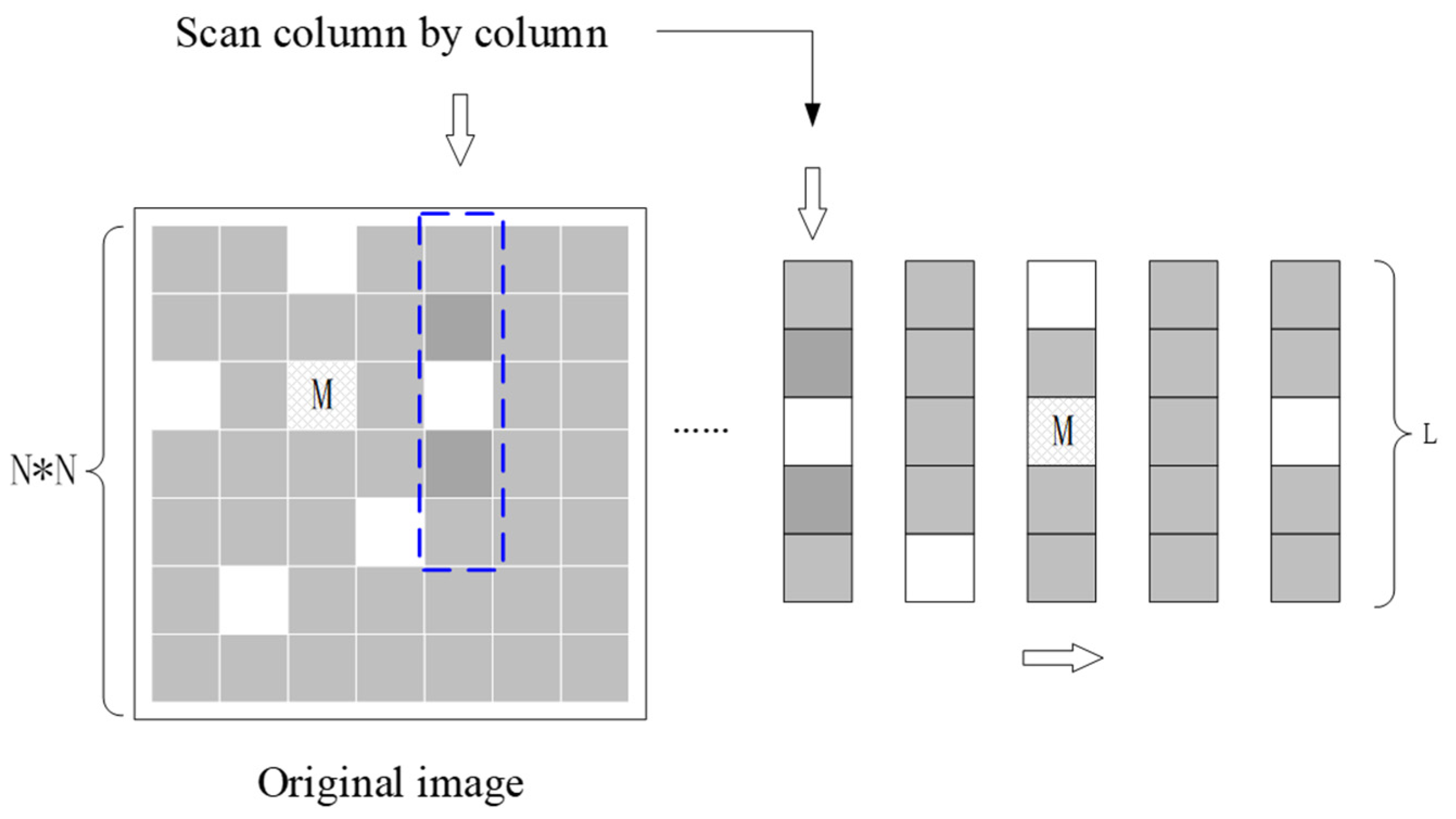
Suppose the original image is an N×N pixel image. Then take the L-dimensional column vector as the unit (N is greater than L) and scan the noise image to be processed from left to right and top to bottom according to the column. This obtains multiple raw pixel block columns and obtains pixel block values, as shown in Figure 3. The original pixel block column including L original pixels, contains both effective pixels and noise pixels. The pixel block value refers to the gray value of the pixel block.

2.1.2. Storing the Original Image

Two copies of the values of the multiple original pixel block columns obtained from the appeal step are made. One for the statistics queue and one for the buffer queue.

2.2. Modular Processing

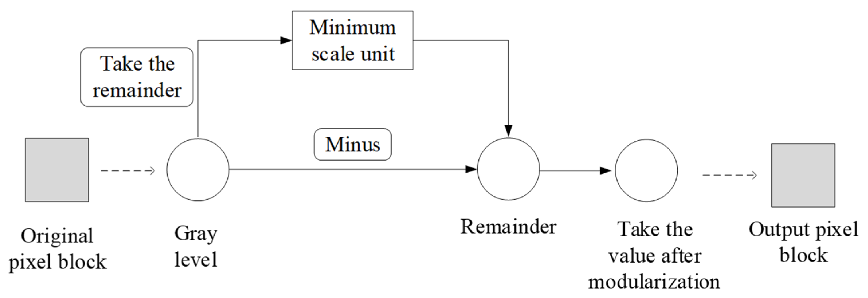
Data columns entering the statistics queue are first modulated. The modularization process is performed to take the remainder between the pixel block value and the preset minimum scale unit and subtract the remainder from the pixel block value, thus obtaining the output value. The details are shown in Figure 4.
The purpose of modularization is to unify points with similar gray values in the image, reduce the impact of details and small changes on noise recognition, increase the recognition rate of effective pixel blocks, and thus improve the recognition of noise points. As shown in Figure 5, the gray values of pixel block 1 and pixel block 2 are the same after modularization. Therefore, by adjusting the minimum scale unit of modularization, we can reduce the loss of details and improve the ability to recognize noise points. When there are too many details in the image, the minimum scale unit can be adjusted higher. Most details can then be unified and will not be regarded as noise. When there are few details in the image, the minimum scale unit can be lowered. Highlighting the changes in the image can improve the ability to recognize noise.

2.3. Data Frequency Statistics

The modularized data are entered in column order at the end of the statistics queue. The statistics queue is a data window of fixed size (L × L). It is used as a data pool for calculating probabilities. As shown in Figure 5, the window comes in at the end, pops out at the beginning, and follows FIFO (first in and first out), with the pop-up columns discarded to keep the window size constant.
Data entering the buffered data queue do not need to be modularized and are fed directly to the end of the buffered data queue in column order. The buffer data queue is a data storage window with a fixed size of L 2 × L (that is, the quotient of L divided by 2 is rounded up and multiplied by L), as shown in Figure 6. This window is used to store data temporarily, and its output is the central pixel block value of the pop-up pixel block column, that is, the M value in the figure.

2.4. Noise Screening and Processing

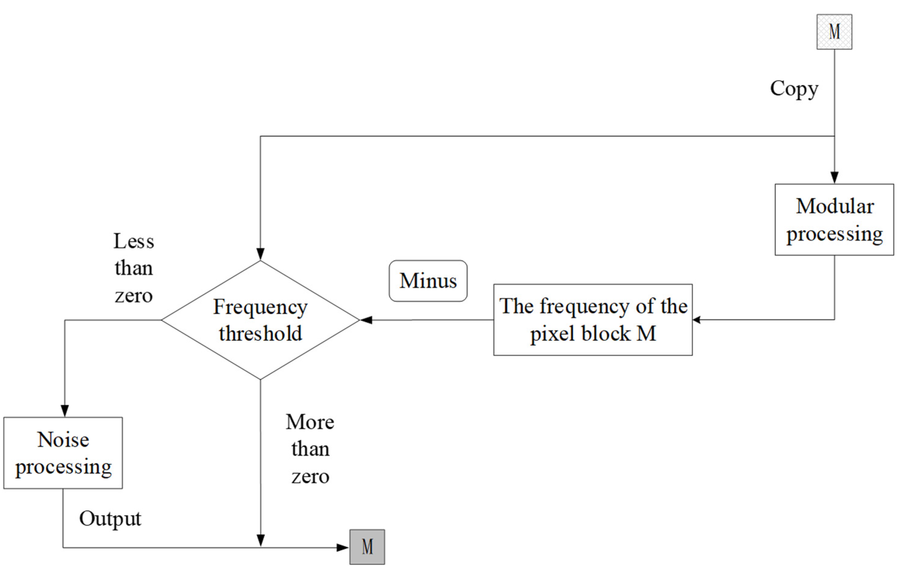
Through the design of the buffer data queue and statistical data queue, it can be seen that output M of the buffer data queue corresponds to the original value of the center point of the statistical data queue. The data transformation of the statistical data queue is equivalent to the statistical data window moving from left to right and from top to bottom for the original image, and the statistical data pool is equivalent to a neighborhood range of M pixel blocks. In addition, the size of the data pool can be adjusted by adjusting the size of L, and the capacity of the data pool can be changed. By calculating the data frequency of the M pixel block in the neighborhood range and comparing it with the preset frequency threshold, the noisy pixel blocks and effective pixel blocks can be separated. The noisy pixel blocks are processed separately to achieve the denoising function, as shown in Figure 7.

2.4.1. Noise Screening

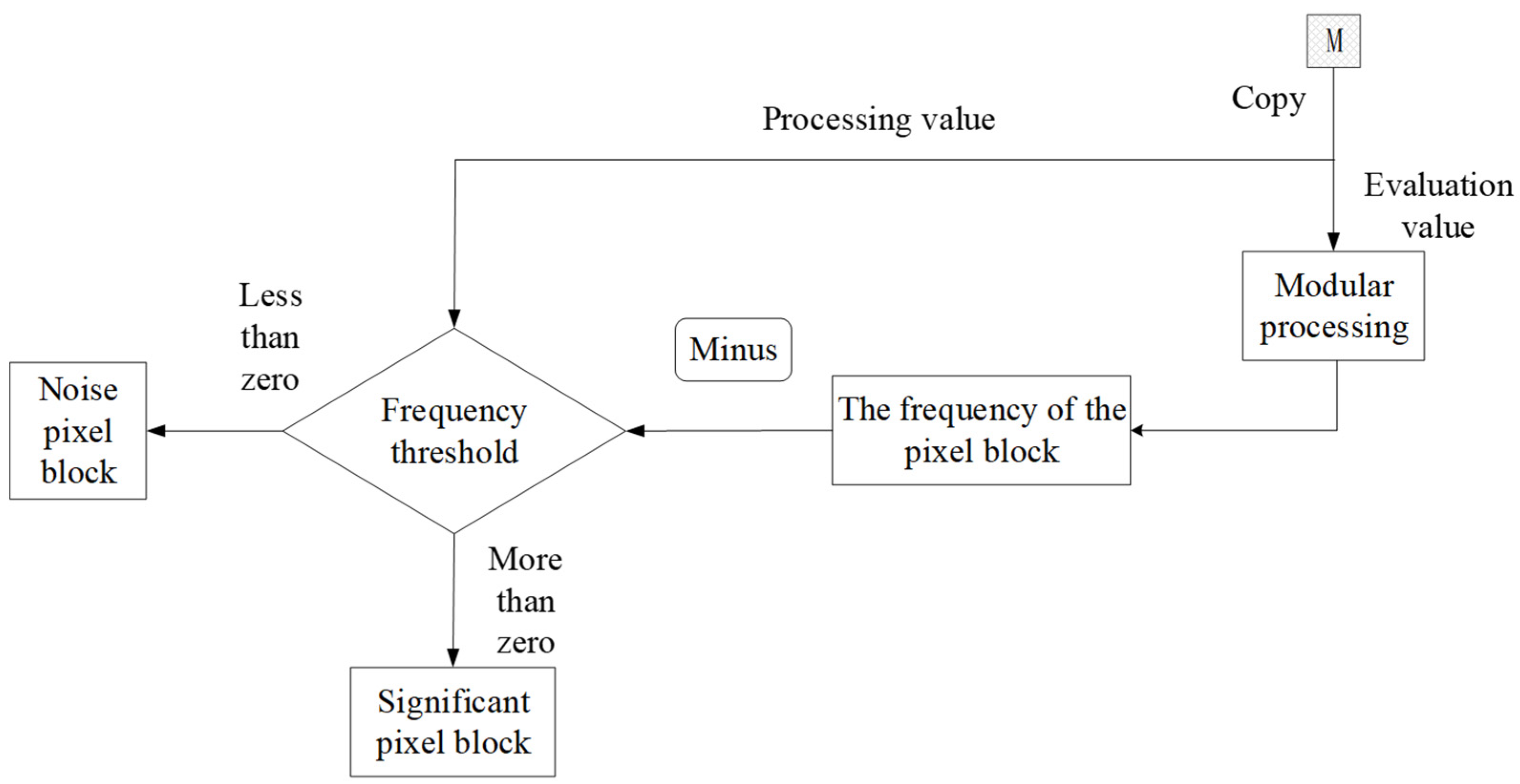
The output, M, of the buffer data pool is first reproduced into two copies, one for processing and one for evaluation. Through the relationship between the buffer data queue and the statistical data queue, the value of output M after modularization is the value of the center point of the statistical data queue. Therefore, M is first modulated and then the number of its values that have the same value as in the statistical data queue is counted, and the ratio is processed with the total number of values in the statistical data queue to generate the data frequency value. When comparing data frequency with a preset data frequency threshold, if the evaluated data frequency is not lower than the preset data frequency threshold, M is a valid pixel block. When the data frequency is evaluated to be lower than the preset data frequency threshold, M is noise. This is shown in Figure 8.

2.4.2. Noise Processing

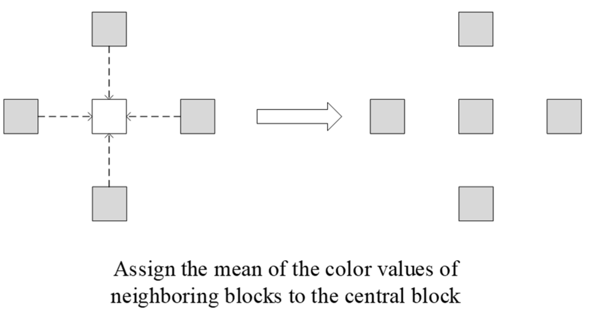
Noisy pixel blocks and effective pixel blocks are separated by the above steps. The noisy pixel blocks are processed separately and the valid pixel blocks are retained. The noise processing method adopts the comprehensive processing method, and the setting method selects the threshold. If noise frequency is lower than the threshold selected by the method, the neighborhood mean method is used, that is, the processing value of noise is changed to the average value of the four adjacent pixel blocks in the original image and then output. See Figure 9 for details.
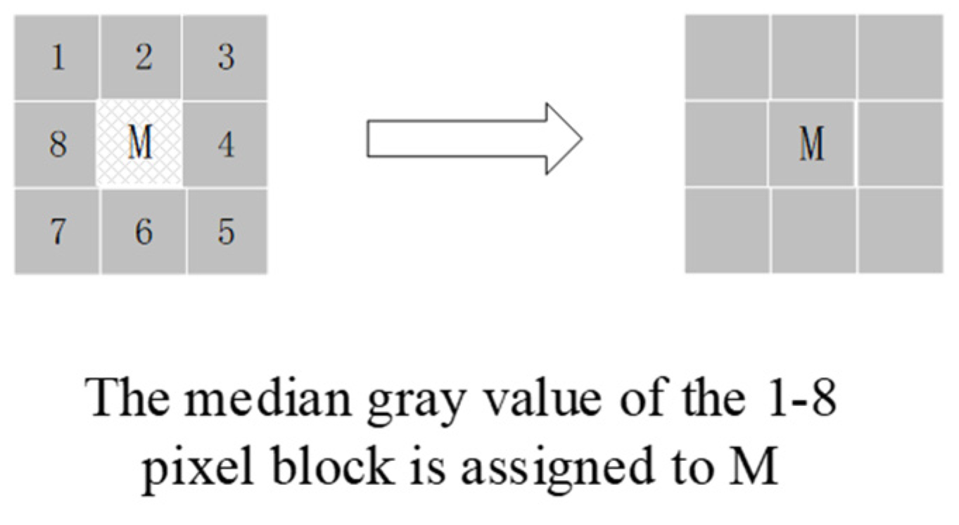
If noise frequency is higher than the threshold selected by the method, median processing is adopted, that is, the noise processing value is changed to the median value of the adjacent eight pixel blocks in the original image and then output. See Figure 10 for details.
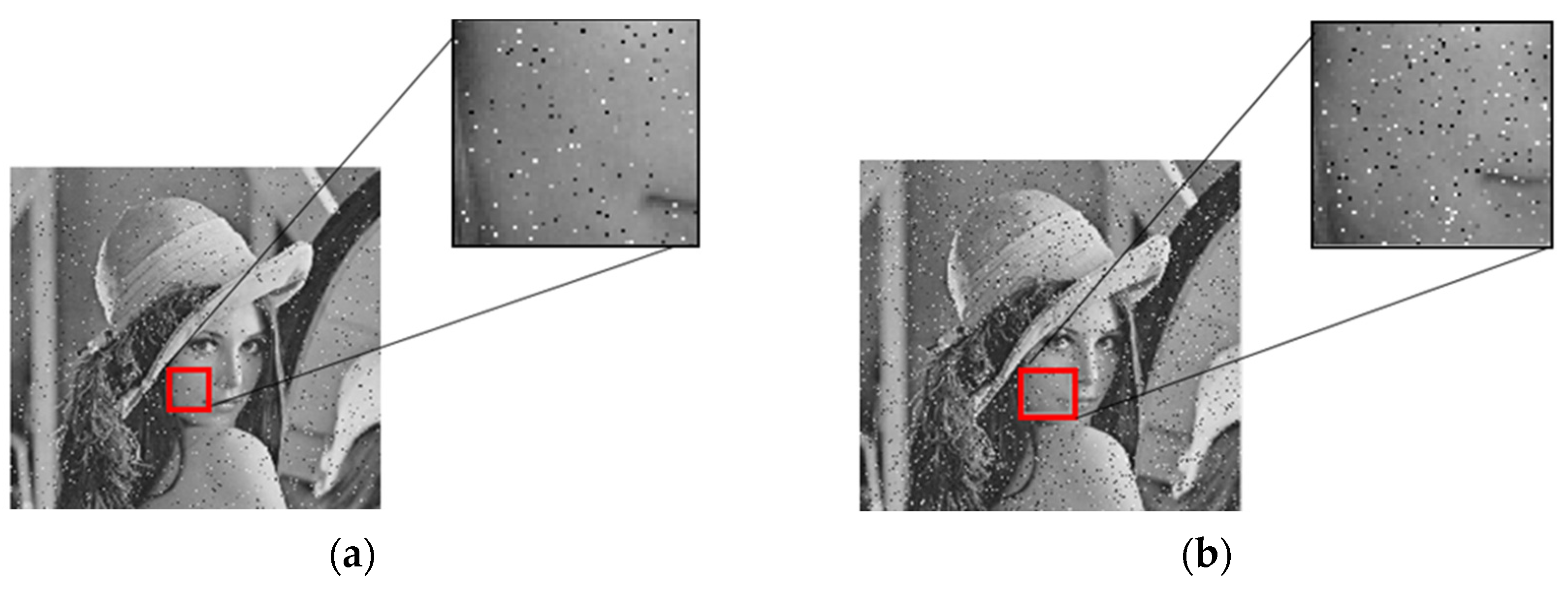
The processing of low-density random value impulse noise is shown in Figure 11a. The median algorithm is likely to output the noise value as the median value after processing, and noise processing has a low fault tolerance rate and poor denoising effect. However, if mean filtering is selected, the image continuity and denoising effect can be ensured to the greatest extent by taking advantage of the fact that the overall frequency of noise points with low density is lower and the probability of adjacent points to noise points is lower. The processing of random value impulse noise with high density is shown in Figure 11b. The noise points are seriously connected, and the use of mean filtering will lead to a mutual influence between the noise points, which will affect the denoising effect. If the median filter is used, the mutual influence of adjacent noise points can be avoided and the denoising effect can be improved.
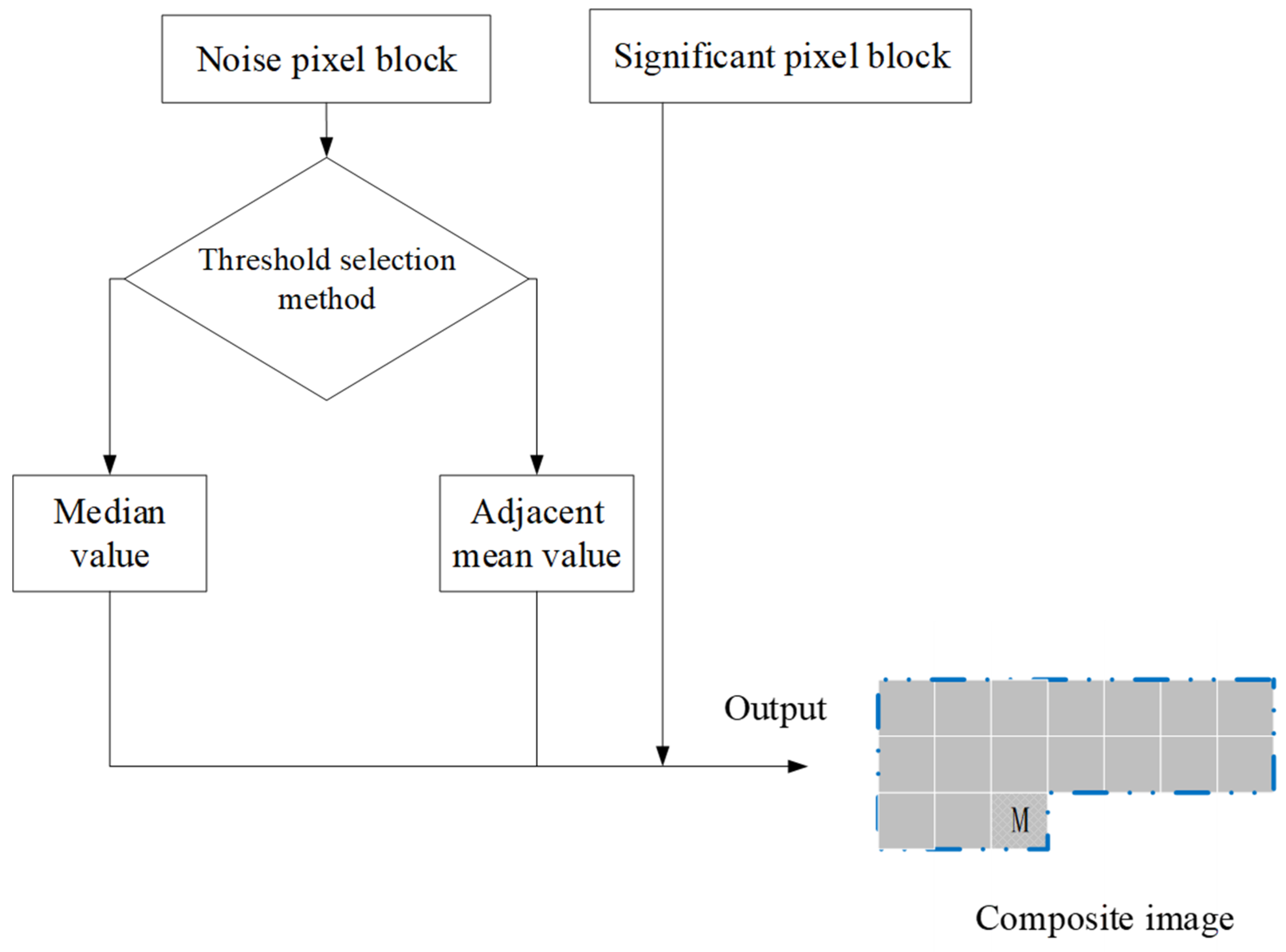
Finally, to maximize the preservation of image details and reduce smear, the processing value of effective pixel blocks will be directly output without processing. The specific noise processing process is shown in Figure 12.

2.5. Composite Image

Finally, each pixel block goes through the above process in turn and outputs several pixel blocks successively to synthesize the final denoised image, as shown in Figure 12. The denoising effect can be adjusted by setting different minimum scale units, statistical data queue window size, preset data frequency thresholds, preset method selection thresholds, and filtering times. For different images and different noise densities, appropriate parameter settings can always be found to achieve as much as filtering during noise processing as possible with the maximum degree of image detail retention. Compared to other filtering methods, the proposed method has the advantages of simple operation steps, shorter operation time, less resource occupation, high operation efficiency, high reliability, simple operation, flexibility, adjustability, and so on.

3. Experiment

3.1. Experimental Conditions

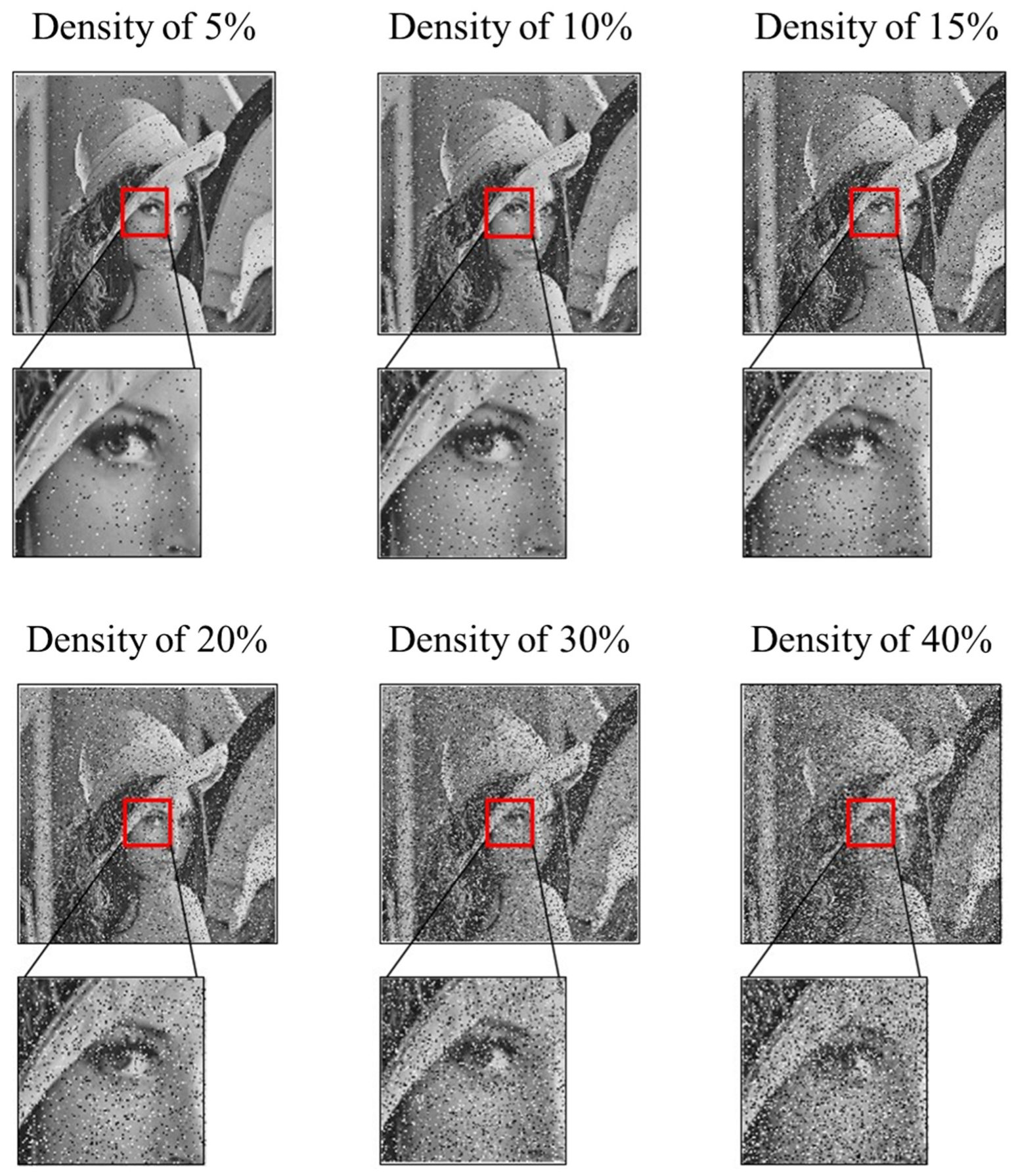
The image used in this experiment is the classic “Lena” gray image, and information for the image is shown in Table 1.
This experiment was carried out on the MATLAB platform, and the added noise was random impulse noise. The low-density noise experiment selected 5%, 10%, and 15% noise, and the medium-density noise experiment selected 20%, 30%, and 40% noise.
Impulse noise with a random value can be adopted into an “impulsenoise()” function, for example, the impulse noise function with a random value of 10% impulse noise density is as follows: “impulsenoise(I,0.1,’random-value’,[0 255])”.
Figure 13 shows the Lena images with impulse noise of different densities.

3.2. Filtering Effect and Comparison

3.2.1. Filtering Methods and Evaluation Criteria

In this experiment, five kinds of filters were used to filter the above random value noise of different density, including the mean filter, median filter, switching median filter, adaptive median filter, and the filtering method in this paper. Moreover, the filtering effects of various filtering methods were evaluated and compared, among which the objective evaluation criteria were peak signal-to-noise ratio (PSNR) and structural similarity (SSIM) [27].
The PSNR is calculated using the following formula:
P S N R = 10 lg ( 255 2 1 M N x = 1 M y = 1 N ( f ( x , y ) f ( x , y ) ) 2 )
where M and N are the length and width of the image, respectively. f ( x , y )   is the gray value of the original image and f ( x , y ) is the gray value of the filtered image. A larger PSNR value indicates a better filtering effect.
Structural similarity (SSIM) is evaluated according to the degree of similarity in local area content between images, which is closer to the subjective evaluation standard. Its calculation formula is as follows:
S S I M ( i , j ) = ( 2 u i u j + c 1 ) ( 2 σ i σ j + c 2 ) ( u i 2 + u j 2 + c 1 ) ( σ i 2 + σ j + c 2 )
In the above formula:
c 1 = ( K 1 L ) 2       c 2 = ( K 2 L ) 2
where i and j respectively represent the image before and after filtering. u i and u j are the average gray value of the image before and after filtering, respectively. σ i and σ j are the variances of the gray value of the image before and after filtering, respectively. K 1 and K 2 are constants much less than 1, which are used to avoid instability when the denominator approaches zero.

3.2.2. Low-Density Random Value Impulse Noise Experiment

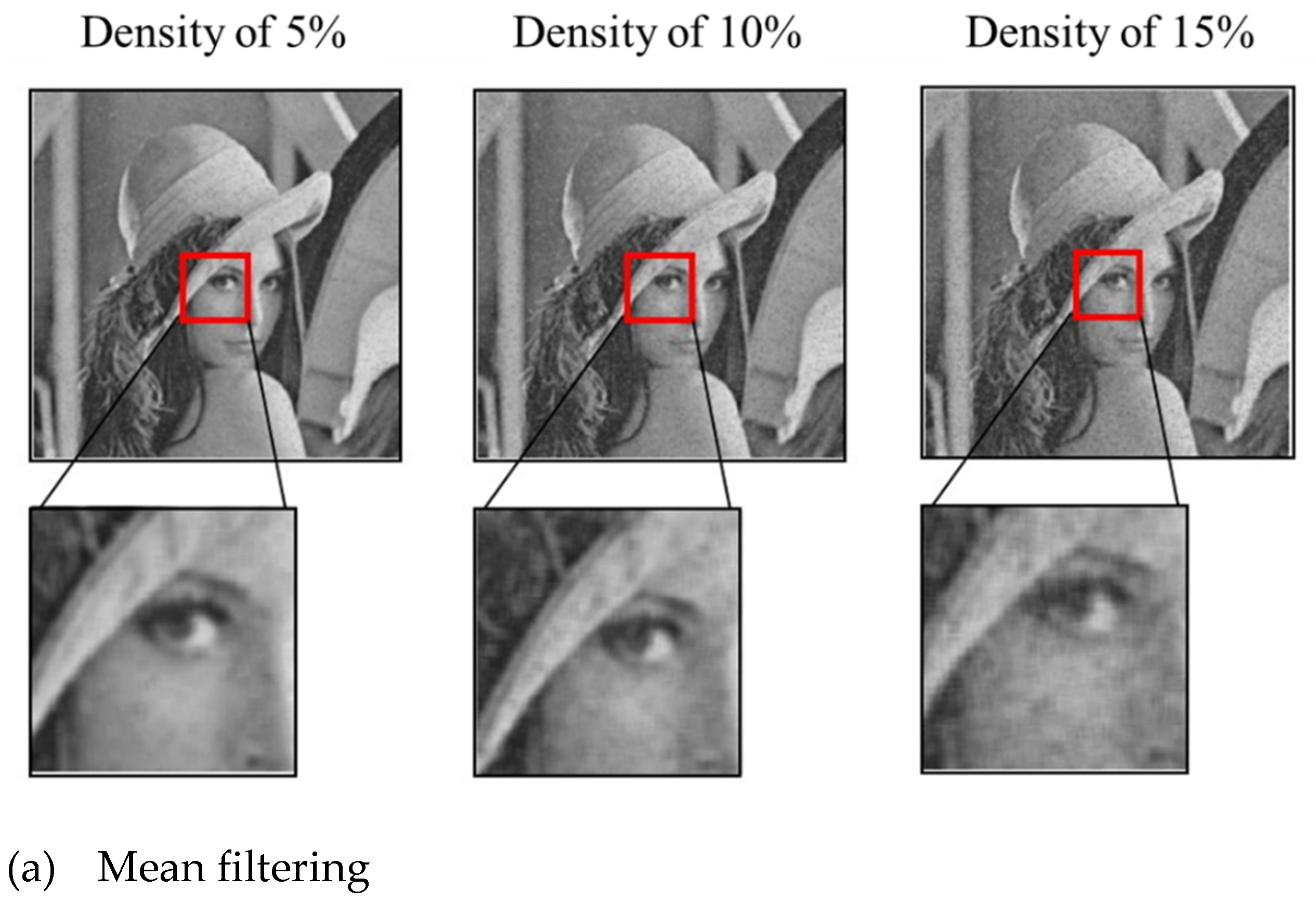
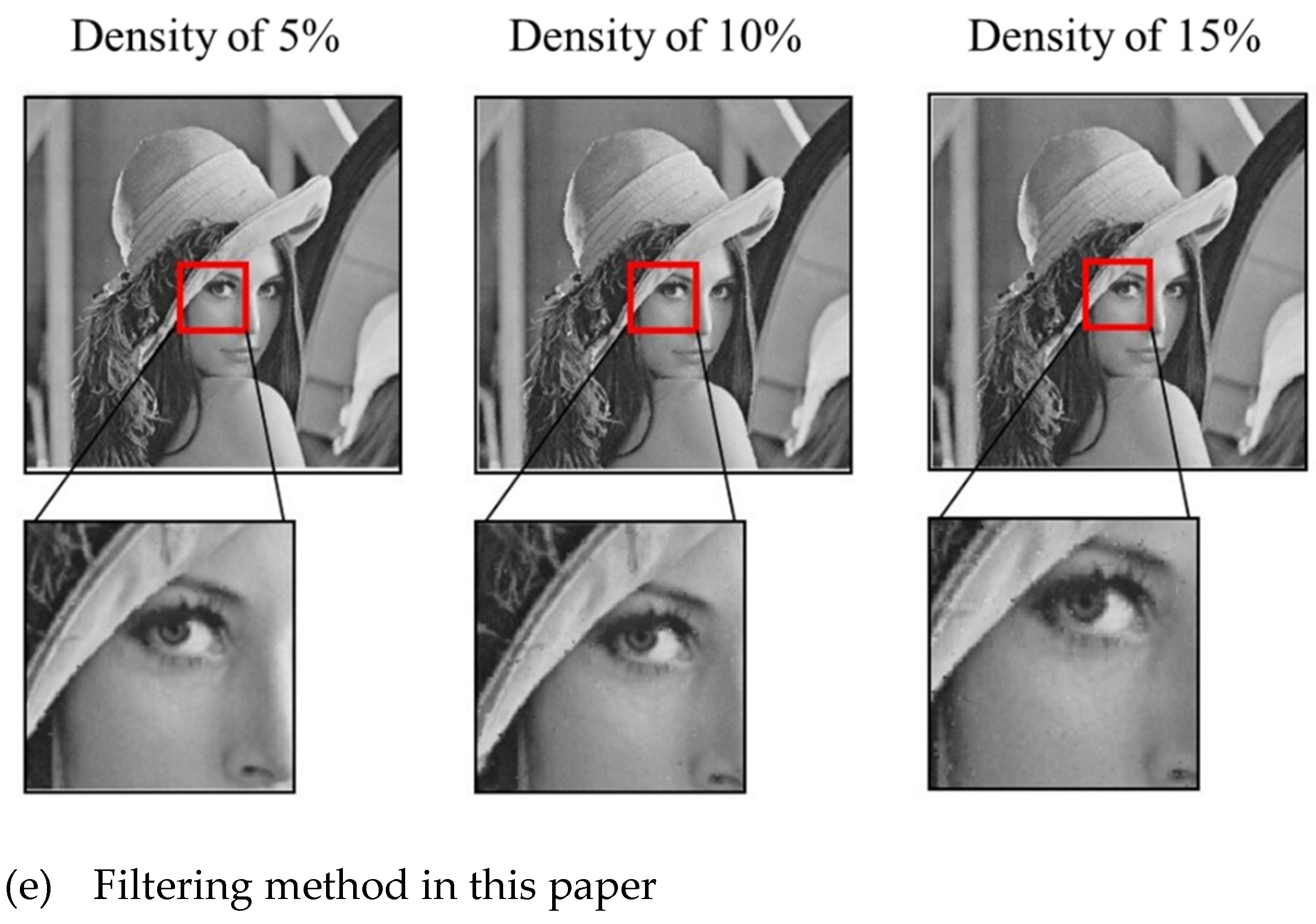
When random value impulse noise density is less than 15%, it is denoted as low-density random value impulse noise. Noise densities of 5%, 10%, and 15% are taken as the experimental objects, and the filtering effects of each filtering method are shown in Figure 14.
In this experiment, a simple mean filtering window of 3 × 3 was adopted for mean filtering. From the overall effect, the image is blurred, although there is no obvious noise trace. However, many of the effective details of the image are suppressed and smoothed and, due to the influence of noise on the mean value, the image after denoising still has many small gray jumps. The shadow of noise can still be seen in the image. This phenomenon becomes serious with increases in noise density, resulting in serious image distortion.
A simple median filtering window of 3 × 3 was adopted for median filtering. From the overall effect, the image appears relatively clear without obvious noise traces. It can be seen from the details that median filtering has a good filtering effect on low-density random impulse noise. Because this is median filtering of the whole image, there is almost no noise omission when noise density is low. However, with increases in noise density, there are some noise omissions, though it is not serious and remains acceptable. In addition, the image denoised by median filtering has the problems of blurring and edge fusion.
A 5 × 5 window was adopted for switch median filtering. The threshold value of the flat area was 4, and the threshold value of the noise area was 20. From the overall effect, it can be seen that noise point filtering was not complete, and noise point traces were obvious. Moreover, it can be seen from the enlarged figure that the recognition rate of switch median filtering for random impulse noise is very low. When noise density is low, there are still a lot of noise points that cannot be identified. With increases in noise density, more and more noise points are missed. Although the filtered image has good detail retention and less edge blur, the overall image quality is poor.
A maximum window of 5 × 5 was set for adaptive median filtering. From the overall effect, it can be seen that noise filtering was not complete, and noise traces were obvious. It can be seen from the magnification that, although the recognition rate of the adaptive median filter for random impulse noise is higher than that of the switched median filter, there are still a lot of noise points that cannot be identified, and this phenomenon becomes more serious with increases in density. Although the details of the filtered image are well preserved and the phenomenon of edge blurring is light, the overall image quality is still poor.
The main parameters of the filtering method proposed in this experiment are set as follows:
  • Window size: 5 × 5;
  • Minimum modular units: 5%—12, 10% and 15%—20;
  • Data frequency threshold: 5%—0.12, 10%—0.16, 15%—0.18;
  • Times filtered: 2;
  • Threshold selected by the method: 5%—0.08, 10% and 15%—0.12.
The overall effect of noise filtering is thorough, the image is clear, and there are no obvious noise traces. From the details, it can be seen that this method has a high recognition rate in terms of noise points and has a better processing effect, and the image details are preserved more completely with a resulting image that is less smooth. With increases in noise density, the filtering effect of the experimental filtering method is still good. It has a better denoising effect on low-density noise points, the filtered image is closer to the original image, and the image quality is generally good.
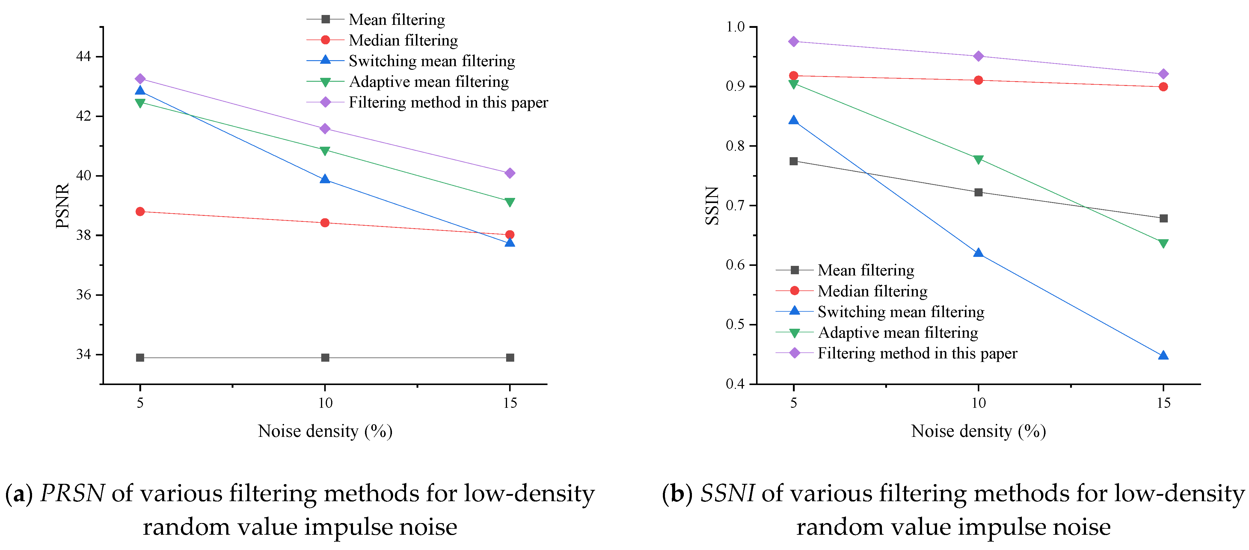
From the objective evaluation criteria, the peak signal-to-noise ratio (PSNR) and structural similarity (SSIM) calculation for each filtering method are shown in Table 2, and the comparison figure is shown in Figure 15.
The larger the PSNR, the closer the SSIM value is to 1, and the better the image filtering quality is. According to the above figure, in the processing of low-density impulse noise and from the perspective of PSNR, the PSNR of the filtering method in this paper was always the highest, followed by adaptive median filtering and mean filtering. With increases in noise density, the PSNR of the switching median filter decreases faster. At 15% noise density, the PSNR of the switching median filter is lower than that of the median filtering method. From the perspective of SSIM, the structural similarity of the filtering method in this paper is still the highest, and that of median filtering is second. With increases in noise density, the SSIM of the proposed filtering method decreases to some extent, but it is still higher than median filtering. The SSIM of the median filter does not change much with increases in noise density (staying above 90%) and has a high degree of similarity to the original image. However, the SSIM of switching median filtering, adaptive filtering, and mean filtering decreases greatly with increases in noise density. The SSIM of the adaptive median filter at 15% noise density is lower than that of the mean filter. The switching median filter decreases the fastest, and structural similarity is even less than 0.5 at 15% noise density. To sum up, under subjective and objective evaluation criteria, the filtering method proposed in this paper has a better denoising effect than other filtering methods for low-density random value impulse noise.

3.2.3. Medium-Density Random Value Impulse Noise Experiment

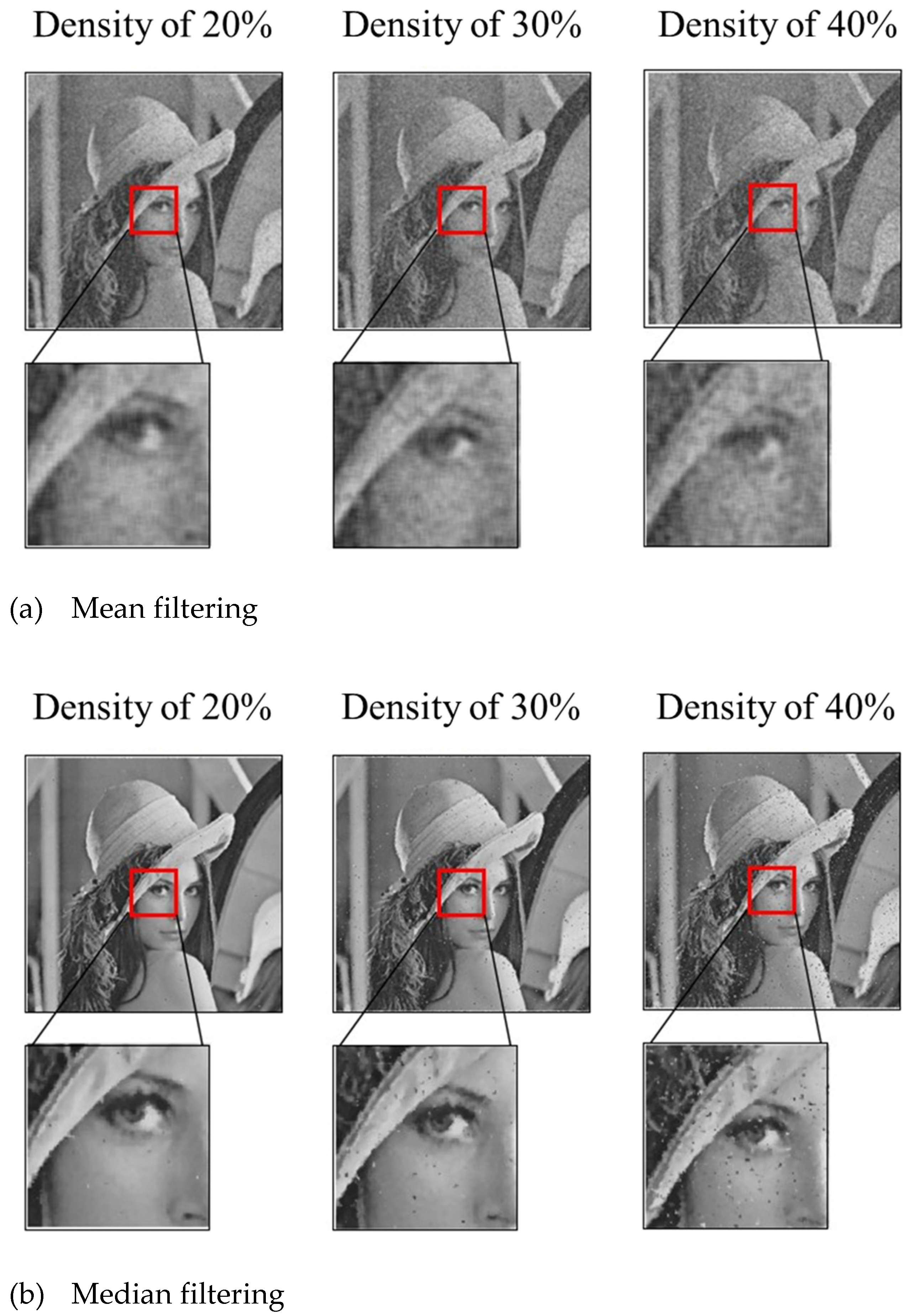
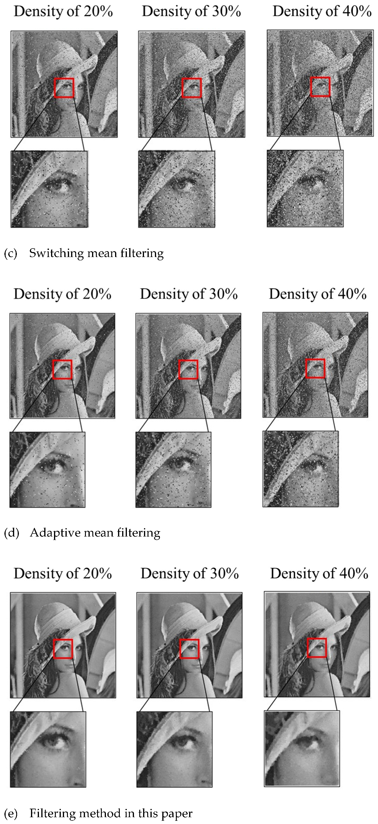
When random value impulse noise density is greater than 15% and less than 50%, it is denoted as medium-density random value impulse noise. Noise densities of 20%, 30%, and 40% were taken as the experimental object. The filtering effect of each filtering method is shown in Figure 16.
In this experiment, a window of 3 × 3 was adopted for mean filtering. From the overall effect, it can be seen that the image is very blurry, and the noise marks are obvious. Many of the effective details in the image are severely suppressed and smoothed. Because noise density was too large, the image details could not be identified, and snowflake noise appeared. This phenomenon becomes serious with increases in noise density, resulting in serious image distortion and a poor denoising effect.
A window of 3 × 3 was adopted for median filtering. From the overall effect, it can be seen that many noise points have been missed in the image. With increases in noise point density, the omission phenomenon becomes more serious, and the image has obvious noise points. From the details, it can be seen that median filtering has a poor filtering effect on random value impulse noise of medium density. As noise density was too large, noise was more likely to be output as the median value; with increases in noise density, this phenomenon is also aggravated. In addition, most of the details in the image after median filtering appear to have been excessively smoothed with blurred edges. Overall, the denoising effect is relatively general.
A 5 × 5 window was adopted for switch median filtering, and the thresholds for the flat area and noise area were 5 and 18, respectively. From the overall effect, it can be seen that the noise filtering effect is very poor, and noise marks are obvious. It can be seen from the enlarged figure that the recognition rate of switch median filtering for random impulse noise is very low and, with increases in noise density, more and more noise points are missed. Image details cannot be identified, thus the denoising effect is very poor.
A maximum window of 5 x 5 was set for adaptive median filtering. The overall noise filtering effect was not thorough, as noise omission was very present. From the enlarged picture, it can be seen that although the recognition rate of the adaptive median filter for random impulse noise was higher than that of the switched median filter, there are still a large number of noise points that cannot be identified, and this phenomenon becomes more serious with increases in density. The details in the filtered image are hard to recognize, the phenomenon of blurred edges is heavy, and overall image quality is not good.
The main parameters of the filtering method proposed in this experiment were set as follows:
  • Window size: 5 × 5;
  • Minimum modular units: 20%—20, 30% and 40%—24;
  • Data frequency threshold: 20%—0.16, 30%—0.24, 40%—0.32;
  • Times filtered: 3;
  • Threshold selected by the method: 20%, 30%, and40%—0.12.
The overall noise filtering effect was more thorough and the image was clear without obvious noise traces. From the details, it can be seen that this method has a high recognition rate for medium-density noise and a good processing effect. However, with increases in noise density, there is a certain blurring phenomenon. Compared to other filtering methods, the blurring is lighter and there is less image smoothing. The denoising effect is good and noises are hardly visible in the details of the image. The filtered image is closer to the original image, and overall image quality is better.
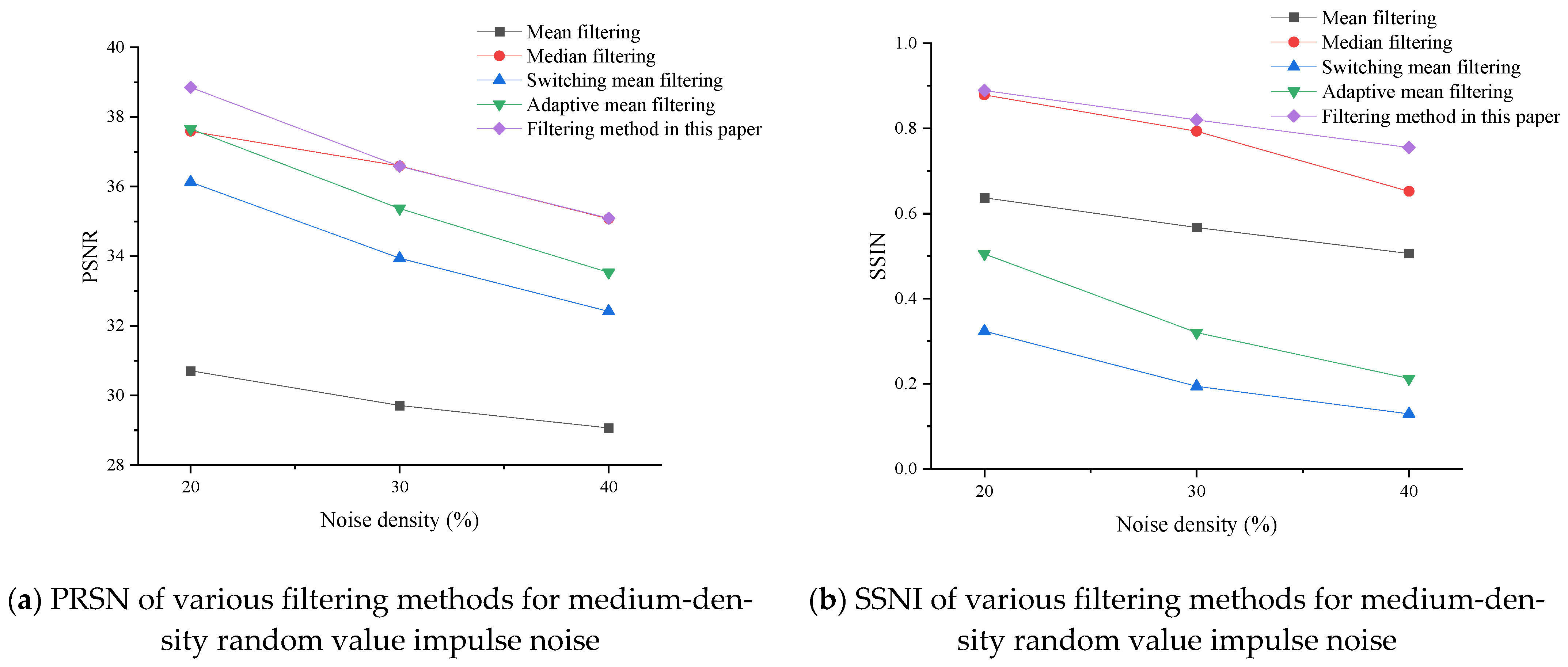
From the objective evaluation criteria, the peak signal-to-noise ratio (PSNR) and structural similarity (SSIM) calculation for each filtering method are shown in Table 3, and the comparison figure is shown in Figure 17.
From the perspective of PSNR, the PSNR of the proposed filtering method is always the highest, followed by median filtering and mean filtering. With the increase in noise density, the PSNR of the switched median filter and the adaptive median filter decreases rapidly, and the median filter is more stable than the proposed filtering method. From the perspective of SSIM, the structural similarity of the filtering method in this paper is still the highest, with median filtering second. With the increase in noise density, the SSIM of the proposed filtering method decreases to a certain extent, but it is still higher than median filtering. The SSIM of the median filter decreases faster with increases in noise density, and the SSIM is lower than 0.7 at 40% density. With the increase in noise density, the SSIM of switching median filtering, adaptive filtering, and mean filtering all significantly decrease by different degrees and their structural similarity is lower than 50%, which shows that filtering quality is poor. To sum up, under the subjective and objective evaluation criteria, the filtering method proposed in this paper has a better denoising effect than other filtering methods for medium-density random value impulse noise.

4. Conclusions

This paper focuses on a filtering algorithm for random value impulse noise and proposes a filtering method based on probability statistics for medium- and low-density random value impulse noise. The main principle is to make use of the fact that the probability of noise points with low and medium density in the processing window is generally less than the probability of effective points. Setting the probability threshold, identifying and separating the noise points, and processing noise points separately while retaining effective points thus achieves the filtering effect. The noise reduction performance of the proposed method and other existing filtering methods, including median filtering, mean filtering, switching median filtering, and adaptive median filtering, are summarized and compared under medium- and low-density random value impulse noise. The main contributions can be summarized as follows:
  • Through the experiment, it can be seen that the proposed method can effectively filter random impulse noise of medium and low density, and better preserve both image detail and quality. The noise reduction effect is superior to other filtering methods at each density, in terms of both subjective and objective evaluation.
  • The structural similarity, SSIM, of the new method proposed in this paper can be maintained above 0.9 under low-density noise conditions and above 0.75 under medium-density conditions, which is much better than other methods. The peak signal-to-noise ratio (PSNR) also demonstrates better stability than other methods at all densities, and the higher the noise density, the more obvious the advantage.
  • The method also has the following characteristics: an adjustable noise reduction effect, high operation efficiency, simple operation steps, shorter operation time, less resource occupation, etc. Therefore, it can realize efficient image processing and has certain practical value.

Author Contributions

Writing and analyzing, Z.L., T.L. (Tao Luo), and Y.L.; conceptualization and supervision, T.G. and T.L. (Tianliang Lin); methodology, T.L. (Tao Luo) All authors have read and agreed to the published version of the manuscript.

Funding

This research was funded by the National Key Research and Development Program (2020YFB2009900), the Collaborative Innovation Platform of Fuzhou-Xiamen-Quanzhou Independent Innovation Demonstration Area (3502ZCQXT202002), the Key Projects of the Natural Science Foundation of Fujian Province (2021J02013), the Natural Science Foundation of Fujian Province, China(2021J01295), and the Open Foundation of the State Key Laboratory of Fluid Power and Mechatronic Systems (GZKF-202026).

Institutional Review Board Statement

Not applicable.

Informed Consent Statement

Not applicable.

Data Availability Statement

Not applicable.

Acknowledgments

Yuanhua Yu from Beijing BinanHX Control Technology Co., Ltd has provided great help in the experimental verification of this study. The authors gratefully acknowledge Yu’s contribution.

Conflicts of Interest

The authors declare no conflict of interest.

References

  1. Tropp, J.A. Just relax: Convex programming methods for identifying sparse signals in noise. IEEE Trans. Inf. Theory 2006, 52, 1030–1051. [Google Scholar] [CrossRef] [Green Version]
  2. Chan, R.H.; Ho, C.W.; Nikolova, M. Salt-and-Pepper noise removal by median-type noise detectors and detail-preserving regularization. IEEE Trans. Image Process. 2005, 14, 1479–1485. [Google Scholar] [CrossRef] [PubMed]
  3. Yi, H. Research on the Improvement of Papper and Salt Noise Identification and Filtering Algorithm. Master’s Thesis, Beijing University of Civil Engineering and Architecture, Beijing, China, 2020. [Google Scholar]
  4. Gupta, V.; Chaurasia, V.; Shandilya, M. Random-valued impulse noise removal using adaptive dual threshold median filter. J. Vis. Commun. Image Represent. 2015, 26, 296–304. [Google Scholar] [CrossRef]
  5. Tukey, J. Nonlinear (Nonsuperposable) Methods for Smoothing Data. In Proceedings of the Congress Record EASCON, Washington, DC, USA, 7–9 October 1974; pp. 673–681. [Google Scholar]
  6. Brownrigg, D.R. The weighted median filter. Commun. ACM 1984, 27, 807–818. [Google Scholar] [CrossRef]
  7. Sun, T.; Gabbouj, M.; Neuvo, Y. Adaptive L-filters with applications in signal and image processing. Signal Process. 1994, 38, 331–344. [Google Scholar] [CrossRef]
  8. Bao, L.; Panetta, K.; Agaian, S. Single Image Based Random-Value Impulse Noise Level Estimation Algorithm. In Proceedings of the Computing Conference, London, UK, 10–12 July 2018; pp. 1306–1318. [Google Scholar]
  9. Yinyu, G.; Kim, N. A Study on Image Restoration Algorithm in Random-Valued Impulse Noise Environment. J. Inf. Commun. Converg. Eng. 2011, 9, 331–335. [Google Scholar] [CrossRef] [Green Version]
  10. Liu, S.; Yu, Z.D. An Improved Method of Switching Median Filter. Microcomput. Appl. 2009, 30, 1–6. [Google Scholar]
  11. Erkan, U.; Gökrem, L. A new method based on pixel density in salt and pepper noise removal. Turk. J. Electr. Eng. Comput. Sci. 2018, 26, 162–171. [Google Scholar] [CrossRef]
  12. Pritamdas, K.; Singh, K.M.; Singh, L.L. An adaptive switching filter based on approximated variance for detection of impulse noise from color images. Springerplus 2016, 5, 1969. [Google Scholar] [CrossRef] [Green Version]
  13. Ashpreet; Biswas, M. Impulse Noise Detection and Removal Method Based on Modified Weighted Median. Int. J. Softw. Innov. 2020, 8, 38–53. [Google Scholar] [CrossRef]
  14. Ma, C.; Lv, X.; Ao, J. Difference based median filter for removal of random value impulse noise in images. Multimed. Tools Appl. 2019, 78, 1131–1148. [Google Scholar] [CrossRef]
  15. HosseinKhani, Z.; Hajabdollahi, M.; Karimi, N.; Soroushmehr, R.; Shirani, S.; Najarian, K.; Samavi, S. Adaptive Real-Time Removal of Impulse Noise in Medical Images. J. Med. Syst. 2018, 42, 216. [Google Scholar] [CrossRef] [PubMed] [Green Version]
  16. Tan, X.; Jiang, J.; Zha, D. Threshold Switch Filter Designing and its Realization in Image Denoising. Modul. Mach. Tool Autom. Manuf. Tech. 2011, 10, 49–52. [Google Scholar]
  17. Wenjuan, L.; Jun, C.; Yonggang, Z.; Xinmin, S. Research of Medical Image Denoising Based on Improved Weighted Mean Filtering. J. Liaoning Univ. (Nat. Sci. Ed. ) 2022, 49, 30–35. [Google Scholar]
  18. Zhang, S.; Karim, M.A. A new impulse detector for switching median filters. IEEE Signal Process. Lett. 2002, 9, 360–363. [Google Scholar] [CrossRef]
  19. Aizenberg, I.N.; Butakoff, C. Effective impulse detector based on rank-order criteria. IEEE Signal Process. Lett. 2004, 11, 363–366. [Google Scholar] [CrossRef]
  20. Peng, Q.; Runtao, D. Ordering Threshold Switching Median Filter. J. Image Graph. 2004, 9, 412–416. [Google Scholar]
  21. Zhenggeng, Q.; Shaoqing, N. Research on an Improved Adaptive Weighted Median Filtering Algorithm. Comput. Technol. Dev. 2018, 28, 86–90. [Google Scholar]
  22. Tsuda, K.; Fujisawa, T.; Ikehara, M.; IEEE. Random-valued Impulse Noise Removal Using Non-local Search for Similar Structures and Sparse Representation. In Proceedings of the International Workshop on Advanced Image Technology (IWAIT), Chiang Mai, Thailand, 7–9 January 2018. [Google Scholar]
  23. Jin, Q.; Bai, L.; Grama, I.; Liu, Q.; Yang, J. Removing Random-Valued Impulse Noise with Reliable Wight. Inverse Probl. Imaging 2020, 14, 171–203. [Google Scholar] [CrossRef] [Green Version]
  24. Peixuan, Z. A New Adaptive Weighted Mean Filter for Salt and Pepper Noise. Master’s Thesis, East China Normal University, Shanghai, China, 2015. [Google Scholar]
  25. Akkoul, S.; Lédée, R.; Leconge, R.; Harba, R. A New Adaptive Switching Median Filter. IEEE Signal Process. Lett. 2010, 17, 587–590. [Google Scholar] [CrossRef]
  26. Qian, X. Research on Filtering Algorithm of Random Value Impulse Noise. Master’s Thesis, Anqing Normal University, Anhui, China, 2019. [Google Scholar]
  27. Sun, X.; Song, S.G. Median Filter Image Denoising Algorithm under Point Detection. China Comput. Commun. 2019, 2, 52–54. [Google Scholar]
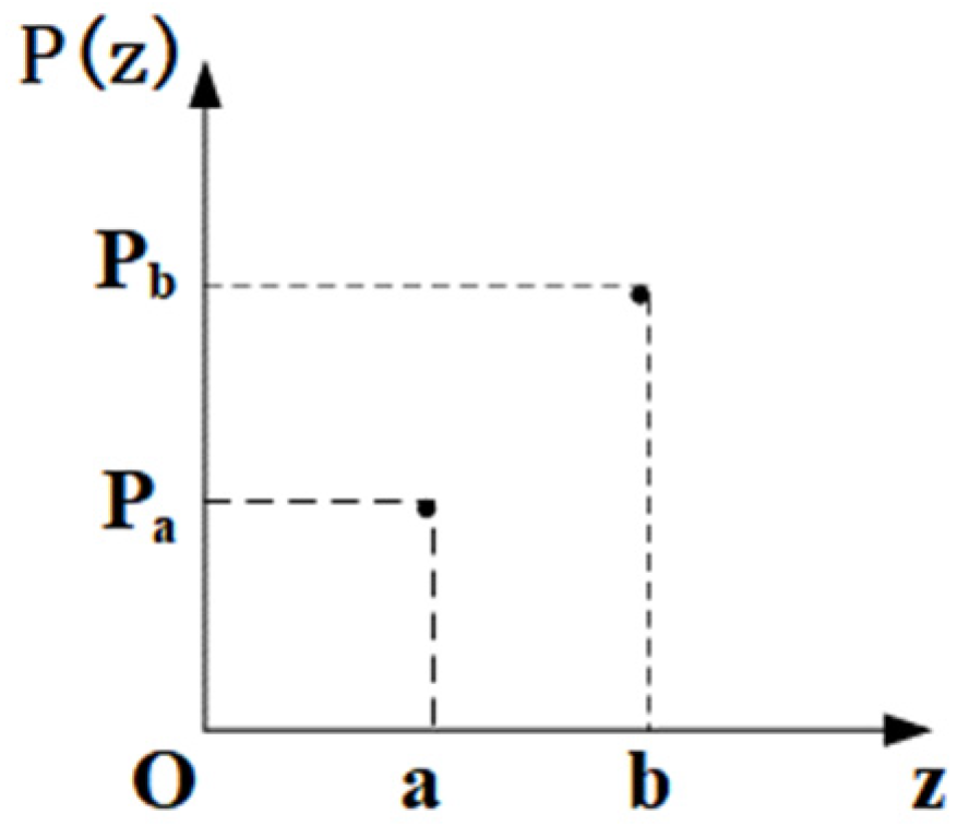
Figure 1. Probability density image of random impulse noise.
Applsci 12 12740 g001
Figure 2. Probability density image of random impulse noise.
Applsci 12 12740 g002
Figure 3. Read the original image (M is the labeled pixel block).
Applsci 12 12740 g003
Figure 4. Modular processing of image data.
Applsci 12 12740 g004
Figure 5. Statistical data queue.
Applsci 12 12740 g005
Figure 6. Buffered data queue.
Applsci 12 12740 g006
Figure 7. The general process of noise processing.
Applsci 12 12740 g007
Figure 8. The process of screening.
Applsci 12 12740 g008
Figure 9. Neighborhood average.
Applsci 12 12740 g009
Figure 10. Median processing.
Applsci 12 12740 g010
Figure 11. Images with different densities.
Applsci 12 12740 g011
Figure 12. The process of noise processing.
Applsci 12 12740 g012
Figure 13. Random value impulse noise images.
Applsci 12 12740 g013
Figure 14. Low-density random value impulse noise denoising images.
Applsci 12 12740 g014aApplsci 12 12740 g014bApplsci 12 12740 g014c
Figure 15. Performance comparison graph of several filtering algorithms.
Applsci 12 12740 g015
Figure 16. Medium-density random value impulse noise denoising images.
Applsci 12 12740 g016aApplsci 12 12740 g016b
Figure 17. Performance comparison graph of several filtering algorithms.
Applsci 12 12740 g017
Table 1. Pictorial information.
Gray ImagePicture SizeContentFormat
Lena512 × 512PortraitBMP
Table 2. Experimental results with low-density random value impulse noise.
Noise
Density
Evaluation
Criteria
Mean FilteringMedian
Filtering
Switching
Mean Filtering
Adaptive
Mean Filtering
Filtering Method in This Paper
5%PSNR33.891538.800542.837642.469843.2589
SSIM0.77500.91820.84220.90530.9756
10%PSNR33.891538.423739.867440.870541.5853
SSIM0.72280.91060.61930.77890.9510
15%PSNR33.891538.020937.725339.144840.0889
SSIM0.67900.89950.44700.63810.9210
Table 3. Experimental results for medium-density random value impulse noise.
Noise
Density
Evaluation
Criteria
Mean FilteringMedian
Filtering
Switching
Mean Filtering
Adaptive
Mean Filtering
Filtering Method in This Paper
20%PSNR30.708737.588336.131637.656938.8521
SSIM0.63700.87880.32370.50490.8890
30%PSNR29.709936.590933.943635.370136.5846
SSIM0.56700.79350.19380.32010.8200
40%PSNR29.065835.075632.416633.533635.0944
SSIM0.50610.65230.12910.21230.7551
Publisher’s Note: MDPI stays neutral with regard to jurisdictional claims in published maps and institutional affiliations.