Article

Experimental and Numerical Study of the Flow Field Structure of High-Speed Train with Different Nose Lengths Head at 15° Yaw

1
Key Laboratory of Traffic Safety on Track, Ministry of Education, Central South University, Changsha 410075, China
2
Joint International Research Laboratory of Key Technology for Rail Traffic Safety, Changsha 410075, China
3
National & Local Joint Engineering Research Centre of Safety Technology for Rail Vehicle, Changsha 410075, China
*
Author to whom correspondence should be addressed.
Appl. Sci. 2022, 12(24), 12712; https://doi.org/10.3390/app122412712
Submission received: 23 October 2022 / Revised: 5 December 2022 / Accepted: 9 December 2022 / Published: 11 December 2022
(This article belongs to the Section Transportation and Future Mobility)

Abstract

:
By using three different head types (5 m, 7.5 m and 10 m nose lengths), the CRH3 (China Railway High-speed 3) flow field structure at 15° yaw was studied through wind tunnel experiments and numerical simulations. The modifications of the aerodynamic coefficients were studied using the Improved Delayed Separation Eddy Simulation (IDDES) method. The results show that the longer the nose length of the tail car, the more it is affected by crosswind. However, the increase in turbulence mitigates the risk of overturning the tail car as the pressure distribution between the train side surface and the underbody becomes more disturbed. The nose length of the head car can affect the position and length of the longitudinal vortex core on the leeward side, thus affecting the lift and side force of each section of the train. The location of the time-averaged vortex core for a 15° crosswind is approximately 0.67H~0.7H high from the ground and 0.65H~0.67H wide from the center of the train. The main frequency of the leeward vortex ranges from 0.1 to 0.3. The transient vibration amplitude at the position of the vortex core is the largest, and the main frequency of vibration is 0.18. The tail car nose length should be properly lengthened since increasing the length of the tail car reduces the negative pressure on the surface of the tail car, thus reducing drag and side force. However, the excessive length of the tail car nose increases the risk of overturning under crosswind.

1. Introduction

Under crosswind, the airflow structure surrounding the train changes, and the train’s aerodynamic force rapidly increases, which affects the running stability and safety. The nose length and nose shape of the train have been demonstrated to have a significant impact on aerodynamics [1,2]. However, the current research mainly focuses on the influence of the yaw angle on the pressure distribution or aerodynamic force in the streamlined head car [3,4,5,6], but the mutual mapping law between the shape of the train and aerodynamic force is unclear.
Random turbulence in crosswinds leads to disorderly turbulence in the flow field around the train, which also changes the train’s aerodynamic performance. Hemida et al. [2] adopted large-eddy simulation (LES) to examine the effect of the nose length on the ambient flow field. The effect of nose length on the aerodynamic property was studied by the DES method, and it was found that the drag coefficient, vortex shedding strength and wake strength decreased with the nose length increase [1]. Niu et al. [7] investigated the effect of nose length on aerodynamic performance using the IDDES method and found that the increase in nose length suppressed the pulsation of drag and lift. In Sun et al. [8], The effects of four types of train nose structures on aerodynamic forces and slipstreams were studied. The effect of three types of tail car on the tail flow was numerically investigated by Chen et al. [9], and found that the spread distribution of wake varied greatly with the length of nose.
Wind tunnel experiment is one of the most convenient ways to study the aerodynamic performances of high-speed trains. Volpe et al. [10] measured the unsteady flow field on the leeward side of the train using Particle Image Velocimetry (PIV) in a wind tunnel. In the studies of Baker et al. [11,12], the wake flow of TGV and ICE train models was obtained through wind tunnel experiments. Bell et al. [13,14,15,16,17] carried out a wind tunnel experiment with large quantities of scaled models, investigated the effect of tail car geometry on the tail vortex structure, and drew many conclusions about wake flow dynamics. Visualizations were conducted in a wind tunnel with a high-speed train (HST) model at various yaw angles [18]. Raghuathan et al. [19] carried out detailed wind tunnel experiments for four different lengths of high-speed trains to investigate the train aerodynamic forces. The aerodynamic characteristics of the train on the slope were analyzed, and the aerodynamic forces and moments of the train increased dramatically [20].
Nevertheless, the aforementioned studies have not yet given a detailed account of the correlation between leeward longitudinal flow characteristics and high-speed trains with different nose lengths through experiments or numerical simulation, especially the influence of turbulence intensity on the leeward longitudinal flow field. Thus, the correlation of aerodynamic lift and side forces with the corresponding leeward longitudinal vortex is beneficial for us to optimize the aerodynamic performance of the train, which motivates the current study. Previous experiments and simulations have used less turbulent flow conditions to study the inflow field changes around high-speed trains and have not yet explored in detail the effect of turbulence on train bypass, and the effect of head geometry combined with turbulence on flow field structure has not been reported.
By aiming at a three-car high-speed train with different nose lengths, this paper numerically investigates the influence of nose lengths on the aerodynamic force. The PIV was applied to research the leeward longitudinal flow dynamics with three different nose lengths trains. Because 15 degrees crosswinds are most common in the nature and the study is universal, the dynamics characteristics of the flow field on the leeward side of the train under 15° crosswind is analyzed, and the influence and mechanism of the turbulent intensity of inflow turbulence on the flow dynamics of high-speed trains are derived at 15° yaw. The results of the study provide some reference for the optimized design of the head car aerodynamic shape with the goal of improving the safety of train operation under crosswind.

2. Experimental

2.1. Experimental Setup and Wind Tunnel

PIV is adopted to capture the velocity fields mainly in the leeward surface of the train. The wind tunnel walls are equipped with optical glass windows on the sides and top for laser shining and camera imaging. The origin of the coordinate system was defined at x = 3.125H (see Figure 1a). The front and back edges of the floor were processed into streamlined lines to reduce the interference with the airflow, see Figure 1, and the test desk was set at 200 mm. Tests were conducted at an oncoming velocity of 30 m/s, corresponding to a Reynolds number ( R e = ρ V H μ ,   3.27 × 10 5 , where μ is the air viscosity coefficient, 1.8 × 10⁻⁵ Pa·s) based on the train height H.
The experiments were executed in an opened-loop, low-speed wind tunnel located at the Central South University, with a length, width and height of 10 m, 1000 mm and 800 mm of the test section. A 1:25 scaled model was chosen, and incoming wind at 15° yaw made that blockage 3.3%. After the grid was installed, the wind speed ranged from 0 to 40 m/s in the test section.
For obtaining the uniform turbulent velocity field, a grid was arranged at the air inlet of the wind tunnel experimental section, with the width of the grille strip b = 60 mm and the net distance between adjacent grilles Mb = 220 mm. The nose point of the train model is 6 m downstream from the grid at a 0° yaw angle. The camera was fixed on the coordinate frame and arranged inside the wind tunnel along the x-direction; the turbulence intensity was 5%.
Specifically, PIV was composed of a synchronous controller, CCD camera, YAG laser, particle generator and computer. The thinnest part of the laser sheet was about 0.5 mm. Air was seeded with tracer particles of approximately 15 μm in diameter. A Nikon Len (80–200 mm lens) was adopted to capture the images. The maximum resolution of the camera was 6600 × 3300 pixels. In the present study, a thin pulsed laser sheet with 500 mJ pulsed energy at wavelength λ = 532 nm and 6 ns pulse duration were used to illuminate the flow region of interest and stimulate the particle scattering light, which was received by the CCD camera at last. Image spatial resolution was 34.82 µm/pixel. The cross-frame time ∆t was 25 ms. The area of each PIV image captured was 250 mm × 150 mm. The displacement error of the tracer particle in both y and z directions was lower than 0.1 pixel. Since each pixel represents 0.063 mm, the uncertainties of the velocity and vorticity for this experiment were about 1.5% and 2.5%, respectively.
The original images were handled by the commercial software Tecplot 360 EX 2017. Before image correlation, a high-pass filter was implemented to emphasize the tracer particle information and to eliminate any inhomogeneous light in the background. The wind speed value determined the interrogation window size to 64 × 64 pixels window size. Overall, less than 2% of the vectors were removed. In order to obtain a quantitative analysis of train leeward vortex evolution by flow field test system.
An experiment was carried out with a cobra probe, which can measure the wind speed below 100 m/s, with an accuracy error of less than 1 m/s, but it cannot measure the reversed flow [15,16,21], see Figure 1b.
The sampling frequency of the cobra probe is 1250 Hz in the wind test, which is recommended a sampling frequency of above 800 Hz by the manufacturer.

2.2. Models

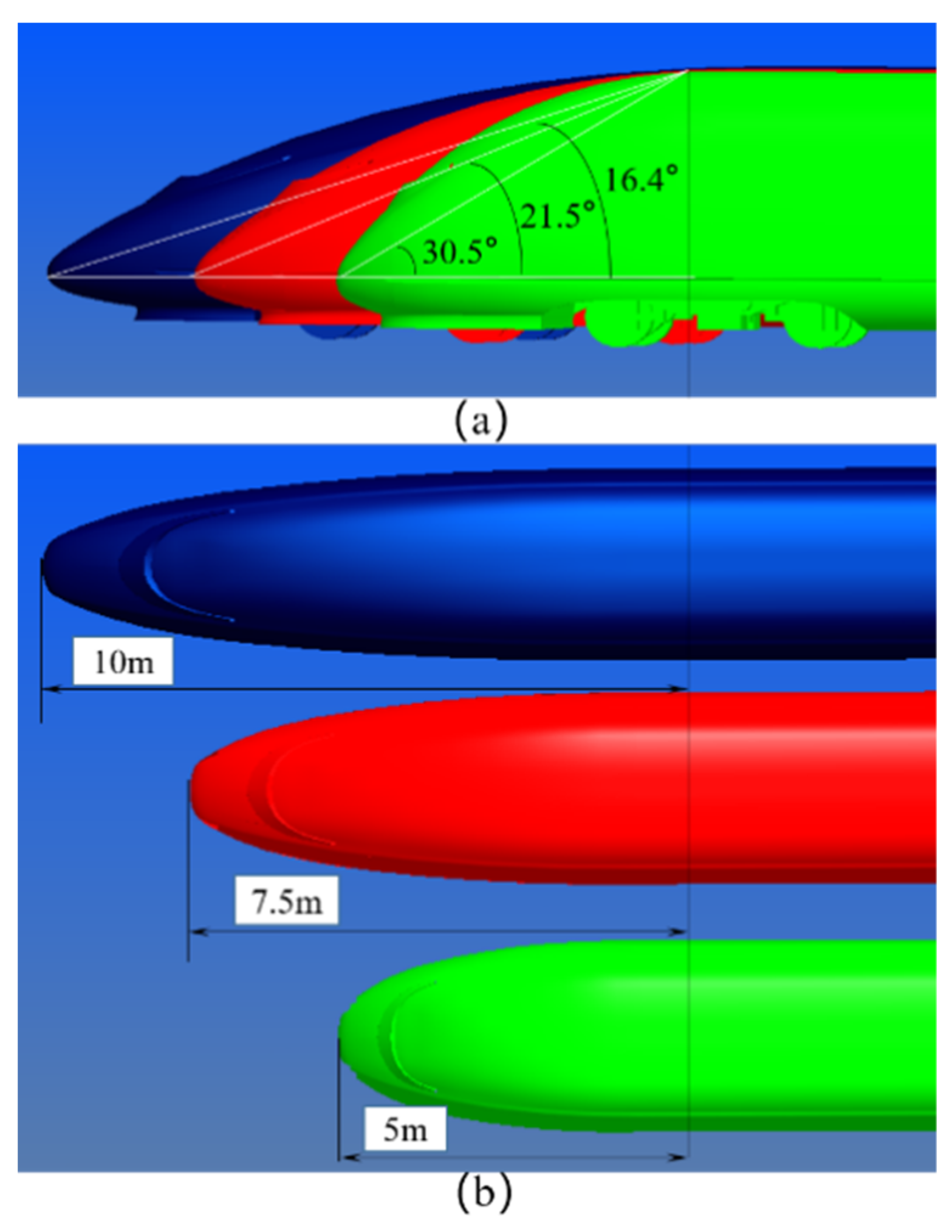
The generic 1/8-th scale CRH3 model with three coaches was adopted in the simulation and is presented in Figure 2. The CRH3 model has been broadly adopted for testing the flow field in various situations. [9,22]. In the current study, in order to focus on the influence of train geometry on the flow field and to better reflect the characteristics of the realistic leeward flow field, bogies were assembled completely in our study. The experimental model was carried at a ratio of 1:25, which resulted in a model height of 0.16 m, width of 0.13 m and length of 2.08 m.

2.3. Roof Boundary Layers

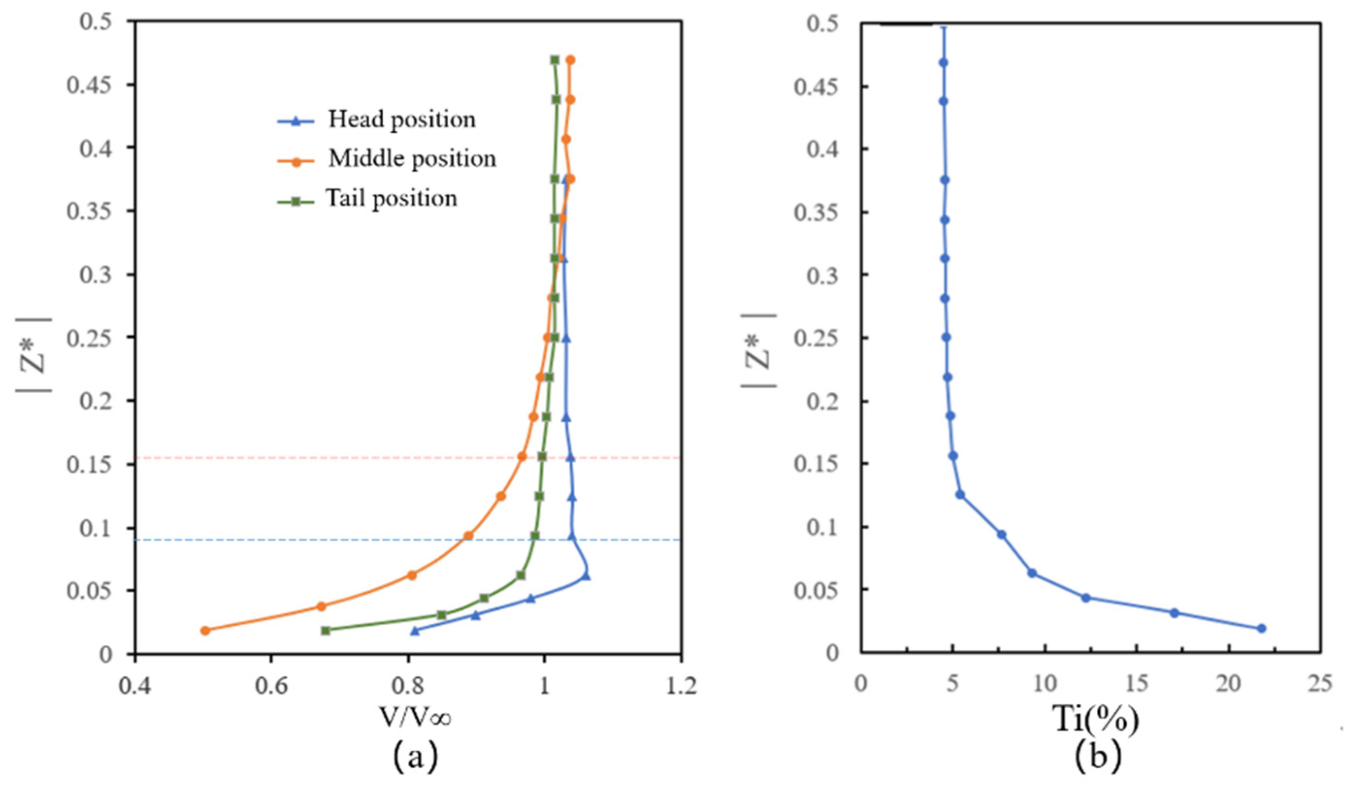
When the nose tip of the mode train was located at x = 6 m, the measured boundary layer thicknesses above the roof of the middle and tail cars of the train were 0.25H and 0.156H, respectively. The difference is that the thickness of the attached layer above the head car is only 0.094H due to the fact that for the cross-section closer to the train nose tip, the pressure on the surface is more influenced by the streamlined nose [23,24]. The roof wind speed fluctuates slightly, showing a trend of increasing first and then unchanged in the height direction (see Figure 3a). In the middle roof position of the train, the variation in turbulence intensity along the height direction is shown in Figure 3b, which reaches a stable value of 5% after 0.156H height position, and the trend is consistent with the results of Zhao et al. [25].
The spatial integral scale of a turbulent flow, i.e., Lx, is defined as Equation (1) [26,27],
L x = 1 σ μ 2 0 R 12 τ d τ
where R12 (τ) is the spatial correlation function of the longitudinal fluctuating velocity, and σ μ 2 is the variance in the fluctuating velocity.
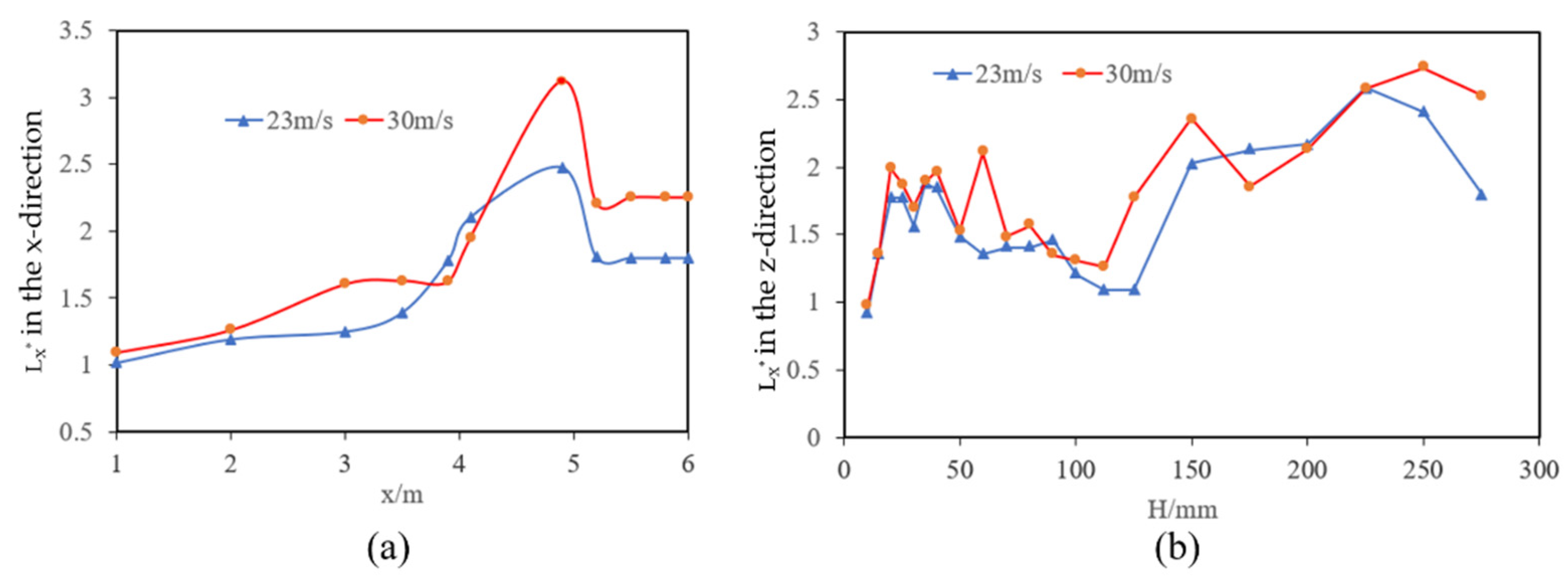
When the incoming wind speed is 23 m/s and 30 m/s, respectively, the integration scale at x = 6 m and h = 275 mm is shown in Figure 4, the normalized turbulence integral scale L x * (=Lx/H) is 1.8 and 2.26, respectively. Where z* is the dimensionless height, z/H. Calculated with V = 23 m/s, which basically conforms to the empirical formula L x M = K x / M 0.6 given by Vita [28] and Roach [29], in this experiment, K = 0.16. The reason for the difference is the non-square cross-section of the wind tunnel for this experiment. Moreover, in the Z-direction, L x * varies between 0.97 and 2.36.

3. Numerical Algorithms

IDDES simulations method of the CFD commercial software STAR-CCM is generated by combining the delayed detached eddy simulation with the wall-modeled large eddy simulation [30]. Therefore, the IDDES is a hybrid model which revised the length scale of the dissipation rate term in equation of the k-ω model [31]. He et al. [32] adopted IDDES, LES and RANS (Reynolds-Averaged Navier–Stokes Equations) to predict the flow field and found that IDDES and LES can well predict unsteady flow but RANS. IDDES simulations method has been successfully applied to various train aerodynamic calculation cases [7,9,32,33,34]. Although LES can also meet the computational requirements, the resource consumption is much larger than IDDES.

3.1. Simulation Models and Computational Cases

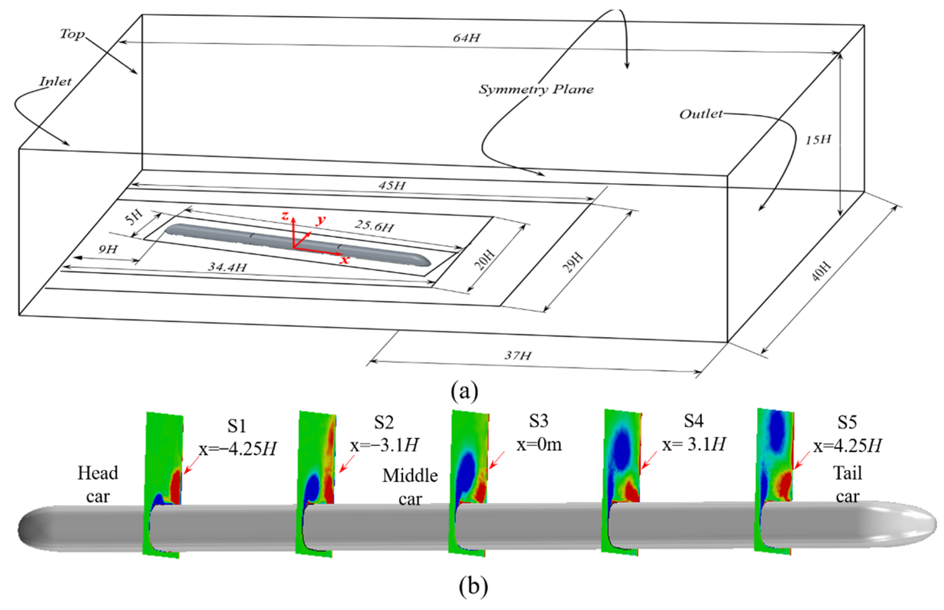
Figure 5 shows the simulation calculation domain and corresponding boundary conditions. The length, width and height of the domain are 64H, 40H and 15H, respectively. The width on the windward and leeward side of the train is 8H and 20H, respectively. The front surface and one side surface of the domain are set to the velocity inlet, inlet speed is 60 m/s, while the back surface and the other side surface of the domain are defined as the pressure outlet, the pressure is 0 Pa. The top surface of the domain is set to symmetry.
The distance from the head nose tip to the inlet plane is 9H, and the distance from the tail nose tip to the outlet plane is 37H. The origin of the coordinate is in the center of the middle car, which is located on the centreline of the calculation domain. The ground is set as fixed ground. We defined the yaw angle β corresponding to the angle between the direction of the resultant wind and train speed. In order to study the structure of the flow field on the leeward side under the crosswind, five cross sections S1–S5 are taken perpendicular to the simulation model, located at x = −4.25H, x = −3.1H, x = 0 m, x = 3.1H and x = 4.25H, respectively (see Figure 5b).

3.2. Computational Grids

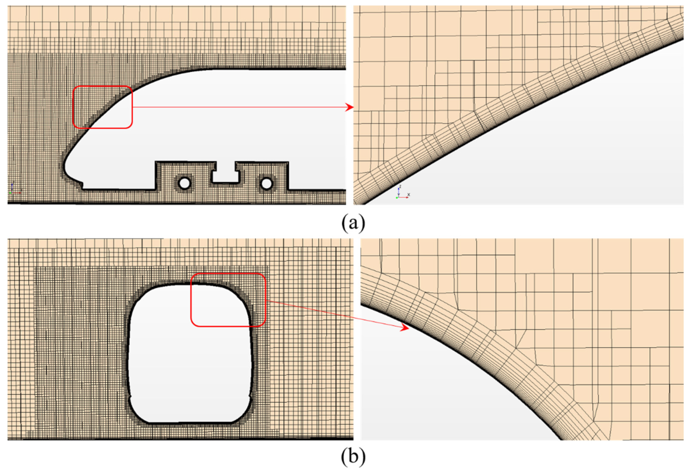
Figure 6 shows the mesh used in the present study. In order to obtain the flow field around the train under high turbulence intensity, three refined areas are arranged around the train body. In order to capture detailed vortex-shedding information on the leeward side, the refined area on the leeward side is wider than that on the windward side. Sub-grade mesh of the head car is shown in Figure 6a. The mesh of the train’s cross-section is shown in Figure 6b. Thirty prism layers of cells are applied to the surface of the train, and the thickness of the grid close to the train body is 5.0 × 10⁻⁵ mm. There is a high-velocity gradient at the surface of the train, so a precise boundary layer grid is set up to solve the complex flow in the boundary layer. The specific values for 7.5 m nose length train’s three types of grids are shown in Table 1. The growth rate of the boundary layer grid is 1.2, and the convergence in a time step is 1.0 × 10⁻³ S. Each simulation used 5 nodes, each node had 48 cores, and one case took 115.72 h.
Figure 7 show the y+ distributions of the head and tail train. Table 2 shows summary of simulations performed at a 15° yaw angle. y+ is less than 1 for both the head and tail car, which meet the calculation accuracy requirements.
Grid independence was verified for the model of Case 2, and the three grids in Table 3 were used to compare the aerodynamic coefficients of the head car. It was found that the results of the medium grid and the fine grid were almost the same, and the maximum difference was less than 3%, indicating that increasing the grid accuracy would not affect the calculation results.

4. Results and Discussion

4.1. The Aerodynamic Force Coefficients and Pressure under Smooth Condition

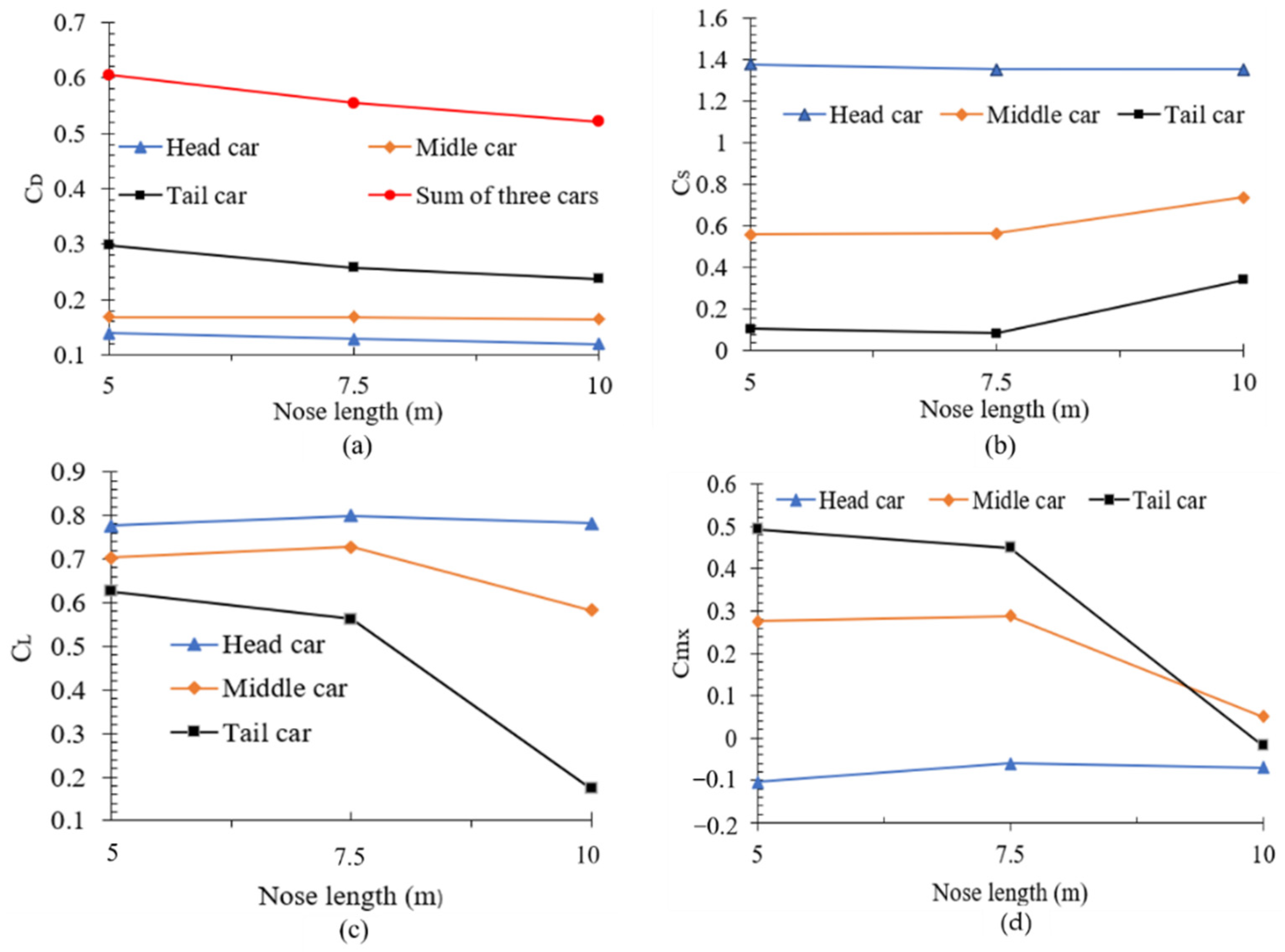
The influence of the nose length of a train on the time-averaged aerodynamic coefficients was investigated. Figure 8 shows the variation curves of the side force coefficient, drag force coefficient, lift coefficient and overturning moment coefficient of the three-section vehicle resistance for different streamlined lengths head. In Figure 8a, as the nose length increases, the drag coefficient of all three trains decreases. The drag coefficient of the three cars decreases by a total of 13.89%, and the drag coefficient of the tail car decreases by 20.43% more than that of the head car decreases by 4.95%, which is contrary to people’s intuition awareness, but consistent with the conclusion of Niu et al. [7] and Chen et al. [1]. From Figure 8b, it can be concluded that the longer the length of the front end of the tail car, the smaller the side force coefficient, and the tail car is more sensitive to the effect of crosswind compared to the head car.
Moreover, it can be seen from Figure 8c,d that the increase in the length of the head car has little effect on both the side force coefficient and the overturning moment coefficient. However, the increase in the length of the tail car has a greater effect on the side force coefficient and the overturning moment coefficient, and the lift and overturning moment coefficients both decrease by 72.35% and 103.63%, respectively.
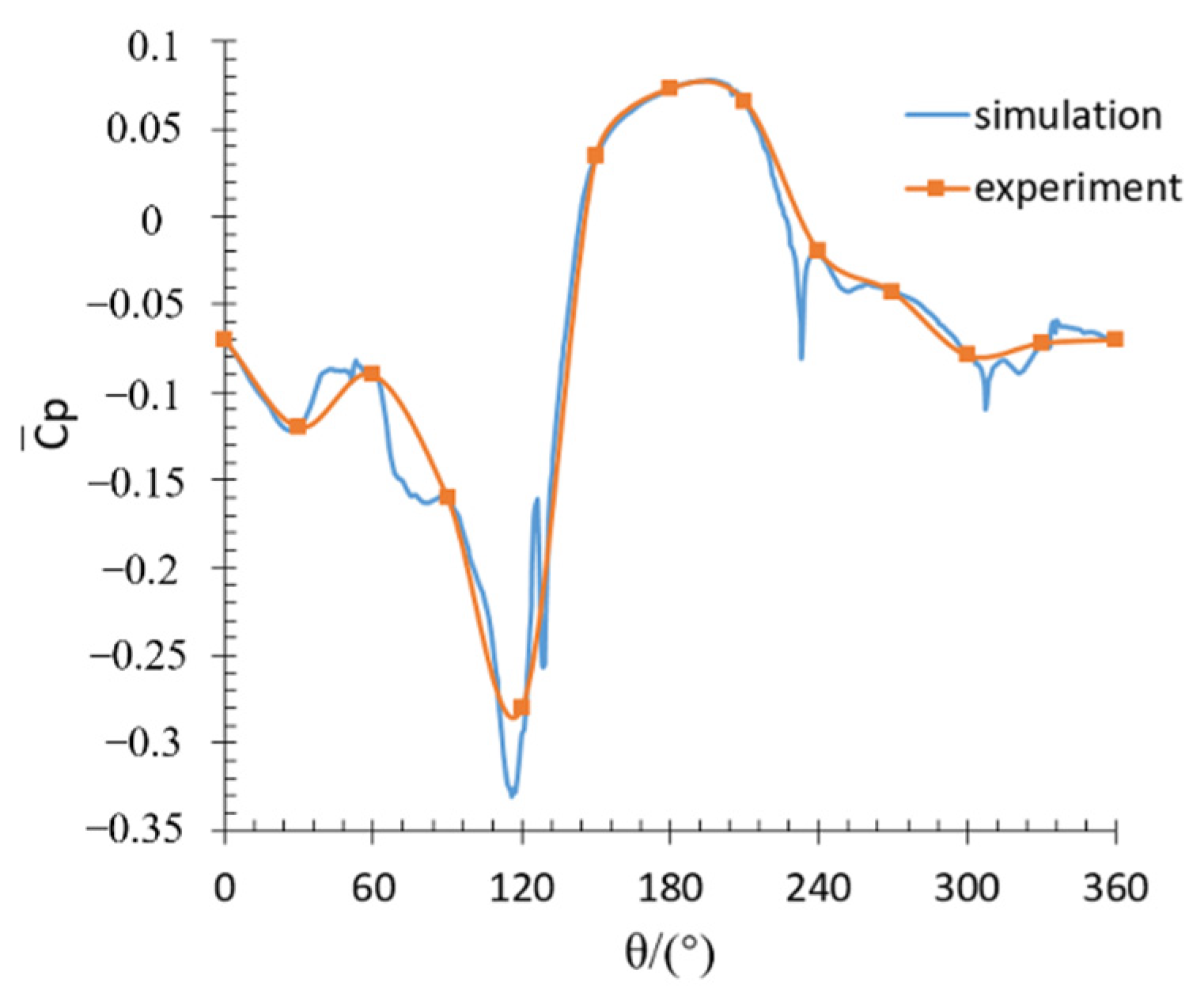
Figure 9 shows the comparison of averaged pressure at the S2 plane of 5 m nose length, and it can also be seen that the pressure differences between the simulation and experiment are small. The maximum difference is 6.7% at 120°.

4.2. Effect of Turbulence

According to Section 4.1, the nose length mainly affects the aerodynamic coefficient of the tail car, which is consistent with the conclusion of Chen et al. [1]. Additionally, the previous scholars [2,13] only studied the influence range of the longitudinal vortex, i.e., until the position of 6H from the nose lip point, the flow field separation and attachment around the tail car are more complicated because both the turbulence intensity of the incoming flow and the nose length of the tail train would affect the aerodynamic performance of the tail car, and the influence on the aerodynamic force of the tail car is not clear.

4.2.1. Pressure Distribution Analysis of the Train Surface

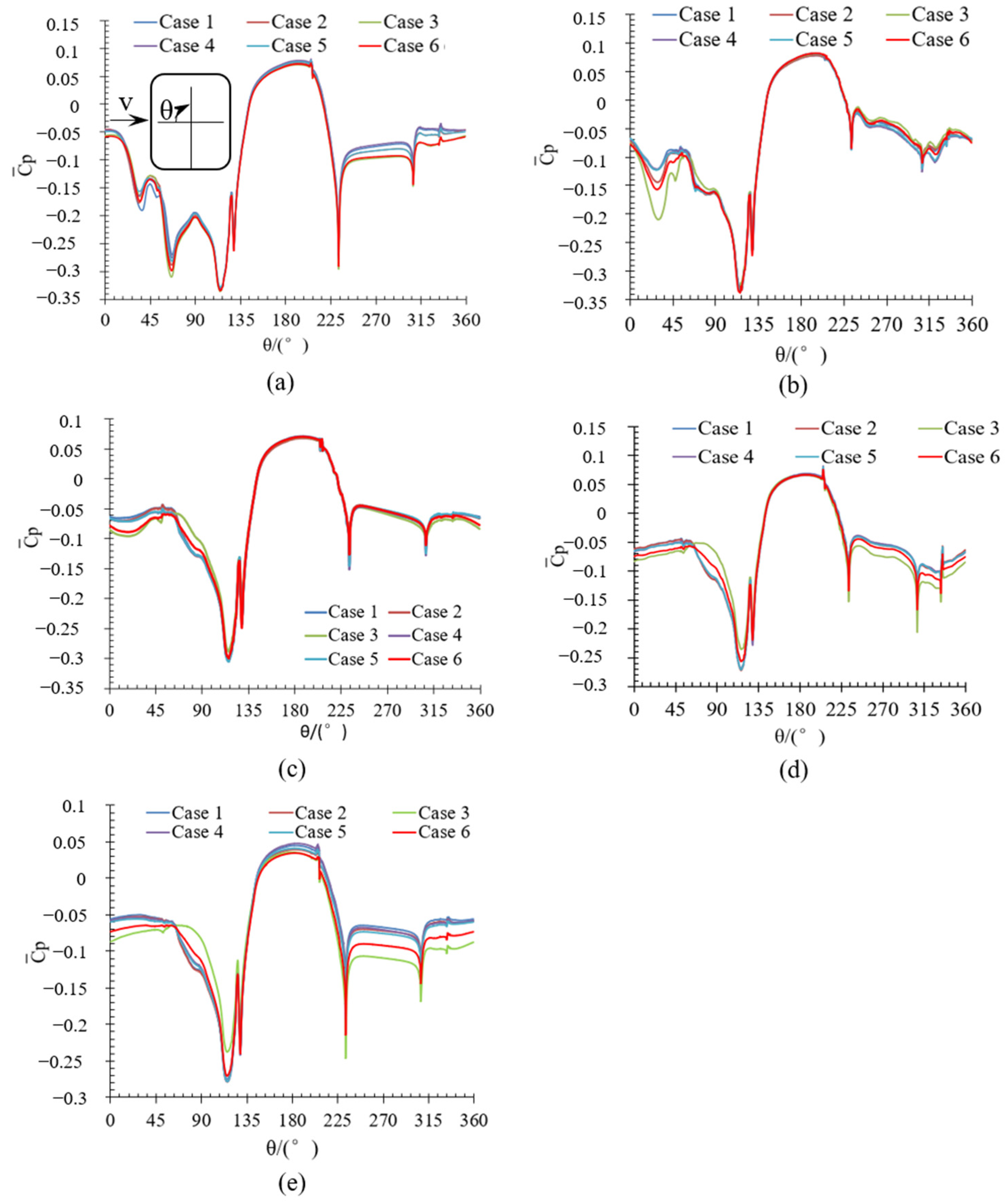
The pressure variation trend around the train body is the main cause of the pneumatic load variation. Figure 10 shows the averaged pressure distribution curves at five cross-sections of the train body surface under different conditions, where the center of the windward surface is the θ origin. The variation in lift coefficient mainly depends on the is reduced, and the roof pressure coefficient no longer drops in a zigzag fashion (as shown in Figure 10a,b) but in a straight line (as shown in Figure 10c–e) the trend of pressure coefficient variation on the top and bottom surfaces (45~135°, 225~315°). From S1 to S5 cross-section, the influence of the streamlining of the head car, the head length increases, and the pressure coefficient difference between the bottom of Case 3 and Case 1 (225~315°) is obvious (as shown in Figure 10a,e). The longer the head length, the greater the negative pressure at the bottom and the greater the negative peak at the corner (θ = 225°). Except for the top and bottom of the tail car, the increase in turbulence intensity is not very obvious to the change in the mean pressure coefficient, which explains the reason why the lift force of the tail car is more affected by the nose length.
The variation in side force coefficient and overturning moment coefficient is mainly influenced by the trend of pressure coefficients on the windward and leeward sides (0~45°, 315~360°). From S1 to S5 cross-section, the windward side is reduced by the streamlined shape of the head, and the pressure coefficient at the roof (0~45°) no longer drops and then rises (as shown in Figure 10a,b) but remains more stable (as shown in Figure 10c–e). With the increase in head length, the negative pressure of pressure coefficient difference between Case 3 and Case 6 windward side of 10 m head becomes lower (as shown in Figure 10c–e). the negative pressure on the windward side of Case 3 is greater than that of Case 6, while the positive pressure on the leeward side is basically the same. Therefore, we conclude that increasing turbulence reduces the Cs of the tail car. The negative pressure on the top surface of Case 6 is greater than that of Case 3, while the negative pressure on the bottom surface of Case 3 is greater than that of Case 6, see Figure 10e. Thus, we conclude that increasing turbulence increases the CL of the tail car. However, for the leeward side of the tail car, the increase in turbulence intensity is not very obvious to the change in pressure coefficient mean value of the leeward side of the remaining cross-section, and the increase in turbulence instead reduces the peak negative pressure of the windward side. The above also explains the reason why the side force coefficient of the tail car is more influenced by the nose length of the tail car.

4.2.2. Force Coefficient

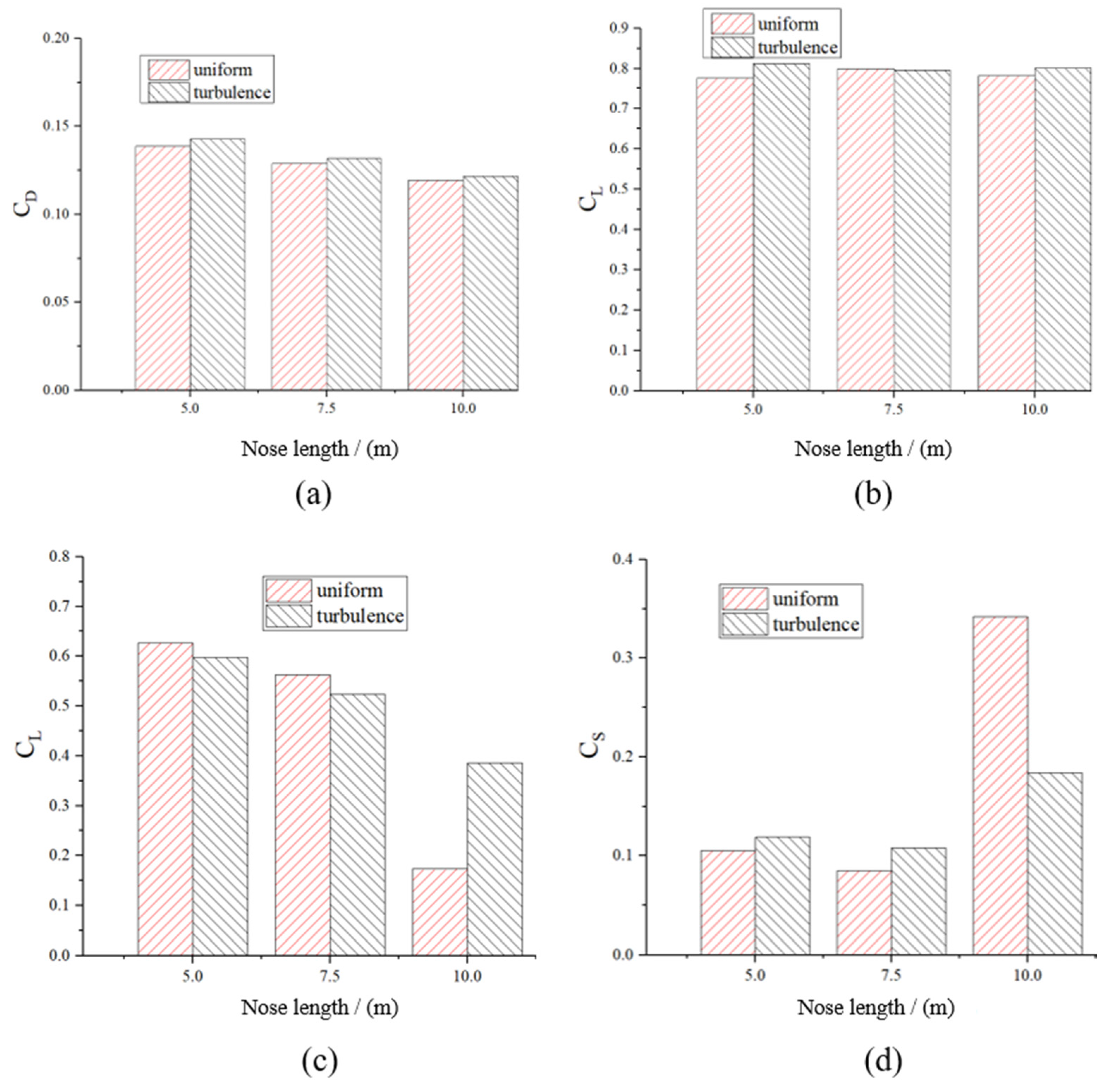
Figure 11 shows the aerodynamic force coefficient of six cases’ head and tail cars with respect to different nose lengths. Overall, the effect of turbulence on the aerodynamic coefficient of the train is greater in the tail car than in the head car.
Turbulence increased drag uniformly for all three heads, increasing by 3% for the 5 m heads and by 2% for the 7.5 m and 10 m heads. Turbulence slightly increases the lift on the 10 m head, decreasing by 0.38% for the 5 m head and by 0.41% for the 7.5 m head. At the same time, it can be seen that the lift coefficients for the 5 m and 7.5 m tail cars slightly decrease with increasing turbulence while the side force coefficients slightly increase. The more obvious changes are the increase of 122.26% in the lift coefficient and the decrease of 46.16% in the side force coefficient for the 10m tail car. Therefore, under the 15° crosswind, the increase in turbulence enhances the safety of the train, especially the tail car enhances the stability of the train under the effect of turbulence, which is contrary to the expected conclusion.
Table 4 shows the standard deviation (SD) of the time-average overturning moment coefficient of trains with different streamlined lengths. The variance in the overturning moment coefficient reflects the amplitude of overturning moment fluctuation. For the same nose length, the tail car has the maximum standard deviation, and the head car has the minimum standard deviation. The main reason may be that there is more vortex shedding occurring on the leeward side under the crosswind. In turbulent conditions, the standard deviation gradually decreases as the nose length increases. Compared with Case 4, the standard deviation of the head car’s overturning moment coefficient, the middle car and the tail car in Case 6 decreased by 20.4%, 2.7% and 24.3%, respectively. Therefore, in turbulent conditions, the longer the nose of the head car is, the smaller the standard deviation of the tail car’s overturning moment coefficient is, and the better the driving stability is.
The longer the head length, the more pronounced the turbulent changes in the overturning moment of the head car. Turbulent intensity increases from 1% to 5%, and when the nose length increases from 5 m to 10 m, the SD increases by 4.95 times to 5.36 times. It is interesting to note that the increase in turbulence changes the amplitude of the overturning moment fluctuation for a train with a 10 m head length from the original maximum SD for the tail car to the maximum SD for the head car.

4.2.3. Lateral Flow Field

As introduced above, the time-averaged flow character is an association of yaw angle and lateral flow field with different nose lengths to vortices. The vortex is identified by the transverse velocity components (v, w) and the vorticity in the yz plane (ωx).
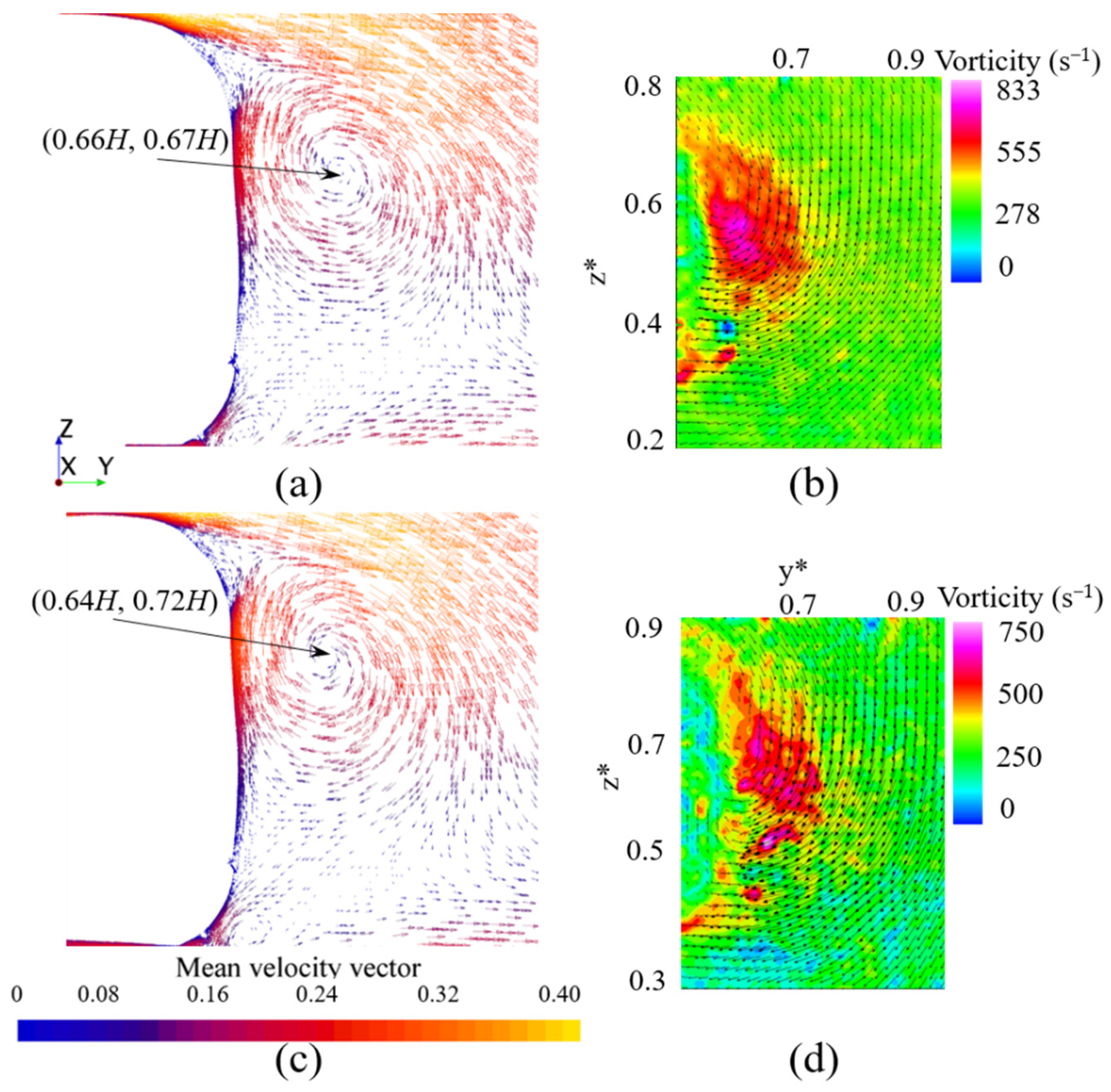
The time-averaged results presented in Figure 12 indicate that the lateral flow field is explained by a large-scaled hairpin vortex; the vortex core is located at 0.67H from the bottom of the train. Where y* (y/H) is the dimensionless width. In Chiu and Squire [35], the leeward flow field is largely insensitive to the stationary floor in the near wake. The crosswind comes over the roof and flows into the leeward side; the flow is locally dominated by rotation, the lateral wind speed reaches the extreme value of about 0.67H from the bottom of the train, and the position of this point gradually rises with the increase in wind speed. When the length of the car head is 5 m and 10 m, the vortex core positions of both leeward vortices change slightly, and the vortex nucleus coordinates of the S2 plane are (0.66H, 0.67H) and (0.64H, 0.72H), respectively. That is, the longer the head of the train, the closer the vortex is to the body and roof of the train in the leeward plane.
The mean velocity vector field in the S2 plane is shown in Figure 12, the U v 2 + U w 2 ¯ value decreases with the increase in the nose length, so the increase in the nose length can appropriately reduce the intensity of the vortex under the crosswind.
The time-averaged vortex field on the leeward side at a wind direction angle of 15° is shown in Figure 12b. From Figure 12b, it can be concluded that the vortex core of the leeward vortex of the train is about located at 0.65H, and the form is a hairpin vortex; under the wind angle of 15°, the longer the length of the streamlined head, the smaller the vorticity on the leeward side.
The identification of vortex and vorticity has been the concern of scholars, and there are three methods for vortex core identification, Q method [36], λ method [37] and △ method [38]. In this paper, we used the λ method [37,39] and applied Equations (2) and (3) for the identification of vortex cores flow.
Γ 1 = 1 N S sin θ M
Γ 2 = 1 N S P M U M U P ·   x P M · U M U P
where Γ 1 is a dimensionless scalar; S is a very small area in the limit (S→0) and for a two-dimensional incompressible velocity field; θM represents the angle between the velocity vector UM and the radius vector PM; S is a two-dimensional area surrounding P, M lies in S; and z is the unit vector normal to the measurement plane. Γ 2 is a Galilean invariant.
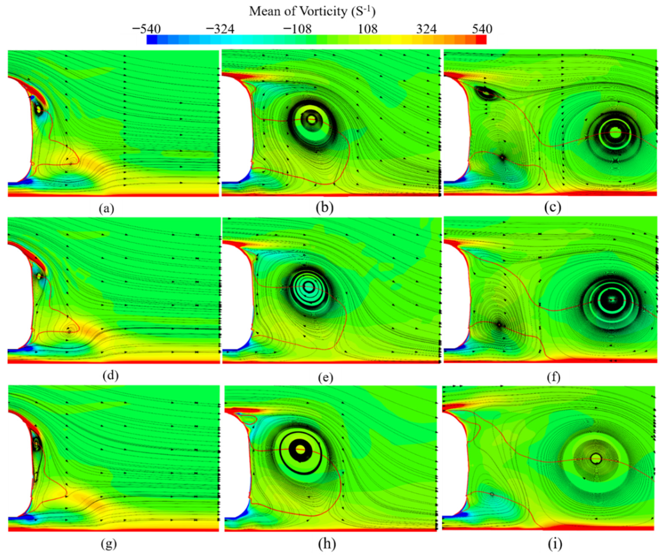
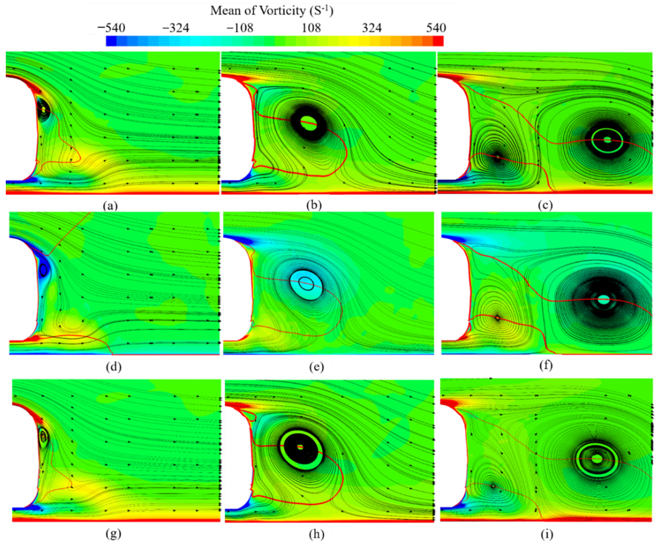
Figure 13 shows the spreading and vertical time-averaged vortex distribution and approximate beam flow lines in the yz plane for S1, S3 and S5 cross-sections under 1% turbulent intensity incoming flow, where the red line is the ensemble line with the spreading flow velocity equal to 0. In Figure 13, small vortices appear at the top of the leeward side of the S1 cross-section, whose vortex field varies less with the increase in the head length, and the position of the vortex field is closer to the train body with the increase in the head length. The vortex scale appearing on the S3 surface in Figure 13 is larger than the S1 surface vortex, which is a longitudinal leeward vortex and is located closer to the train body as the head length increases. On the S5 plane, in Figure 13, in addition to the longitudinal leeward vortex, there are two other vortices on the leeward side, located at the top and bottom of the leeward side, but the top vortex is not obvious in Case 2 and Case 3. Overall, with the increase in the nose length of head car, the vortices affecting both lift and side forces are closer to the car, resulting in a larger aerodynamic SD for the long nose length of head car. Figure 14 shows the mean vortex distribution and approximate beam flow lines in the yz plane in the spreading and vertical directions for the three cross sections S1, S3 and S5 under 5% turbulent intensity incoming flow. Comparison with Figure 14 reveals that the increase in turbulence intensity has less effect on the location of the vortex core on the leeward side of Case 4 and Case 5 because the longitudinal vortices are relatively far away from the bottom vortex core. However, as the streamlined length of the train wake reaches 10 m, the longitudinal vortex in Case 6 is closest to the train body, compressing the bottom vortex. Moreover, because the rotation direction of the bottom vortex is counterclockwise, thus strengthening the counterclockwise moment on the leeward side, the tail car lift force increases and the side force decreases. At the same time, due to the increase in incoming turbulence intensity, the turbulence increases the curvature of the shear layer by interacting with the shear layer separated from the top of the train, which makes the shear layer closer to the leeward side and reduces the side force and overturning moment, which improved the stability of the train. Increasing the turbulence intensity of the incoming wind makes the vortex core of the separation vortex on the leeward side far away from the vehicle body, thus achieving the effect of delayed separation.
According to Figure 13c,f,i, it can be concluded that when the nose length of the tail car gets shorter, the vortex core of the separation flow on the leeward side of the tail car is further away from the vehicle body under 15° crosswind, thus delaying the flow separation on the leeward side.
Comparing Figure 13i with Figure 14i, increasing the turbulence intensity of the incoming wind will make the vortex core of the separation vortex on the leeward side far away from the vehicle body, thus achieving the effect of delayed separation.
Figure 15 shows streamlines projected on the surface of the head train. When the airflow is through the streamlined head, the separation line is marked as SL. Flow separation occurs at the top of the train, followed by turbulent reattachment in a small area on the leeward side. Compared with Case 2 and Case 3, the separation lines at the top and bottom of the leeward side of the head car of Case 1 are farther apart. The separation lines of Case 1 cannot converge at the leeward side of the head car, which also leads to the large negative pressure value at the bottom of the head car of Case1 and the small lift coefficient of the head car. The increase of turbulence intensity has more influence on the lift coefficient of the head car and less influence on the side force.
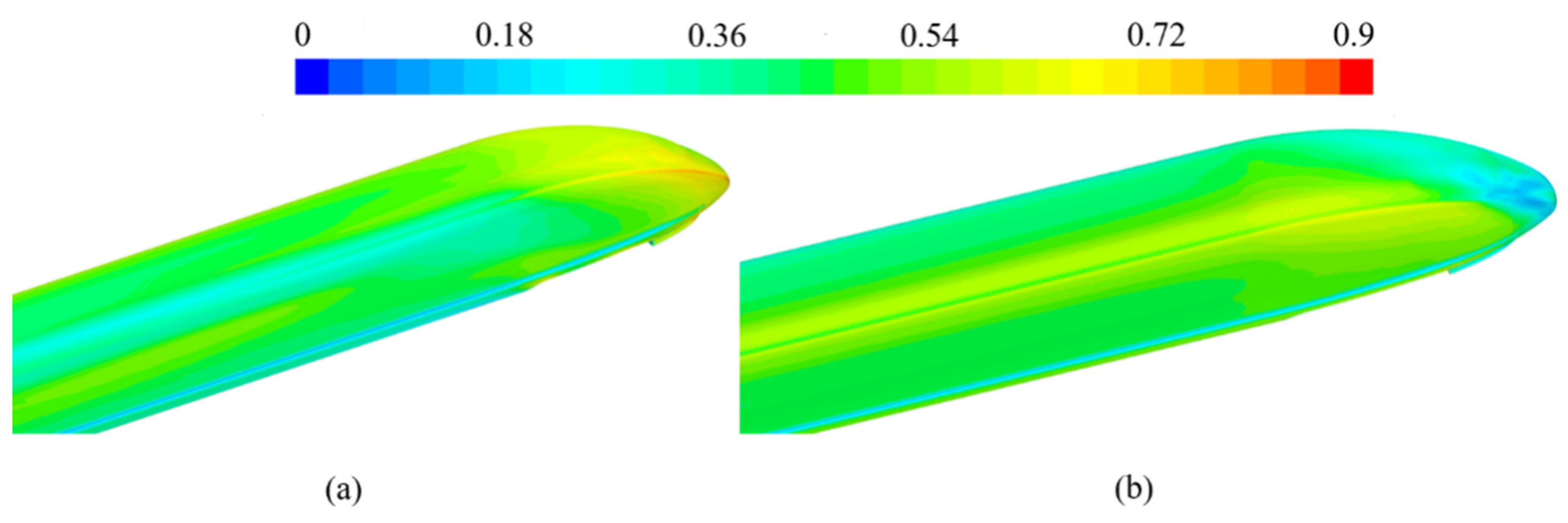
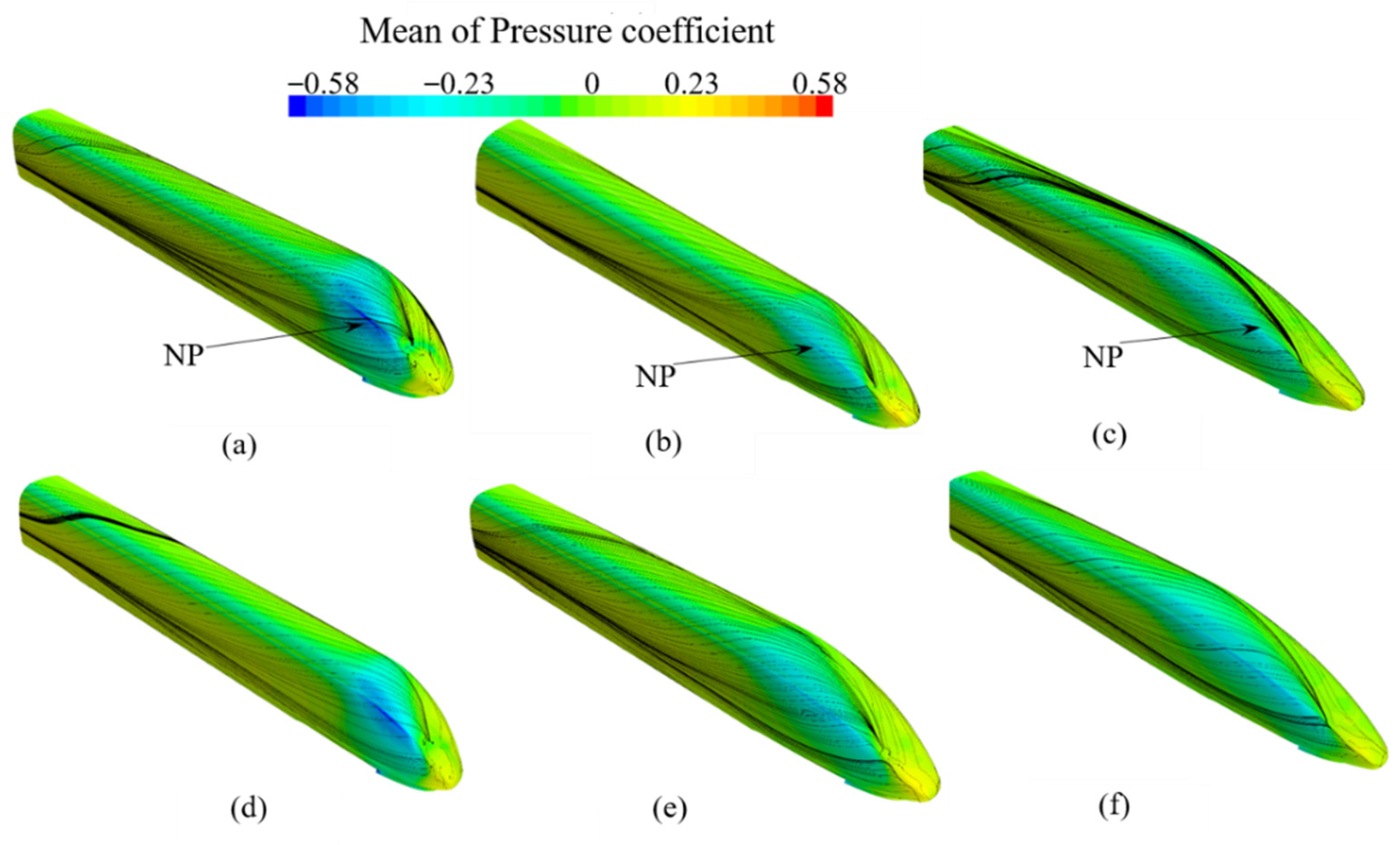
When the air flow past the streamlined tail, the pressure of the train body varies greatly with the length of the tail car, and the pressure decreased and denoted by the NP (negative pressure). As shown in Figure 16, the maximum negative pressure coefficients in the tail car of Case 1, Case 2 and Case 3 are −0.577, −0.444 and −0.382, respectively. The negative pressure area of the tail car is larger, which has an effect on the tail car lift and side force. This is because the negative pressure extremes become smaller as the nose length of the tail car increases. Meanwhile, the enhanced turbulence intensity has little effect on the negative pressure extreme value, as is shown in Figure 16d–f.

4.2.4. The Power Spectral Density or Spectrum

The power spectral density or spectrum Eu is defined as follwed:
E u n = 1 2 π e i n t R u u τ d τ
where R u u τ = u t u t + τ ¯ , and τ is the time lag.
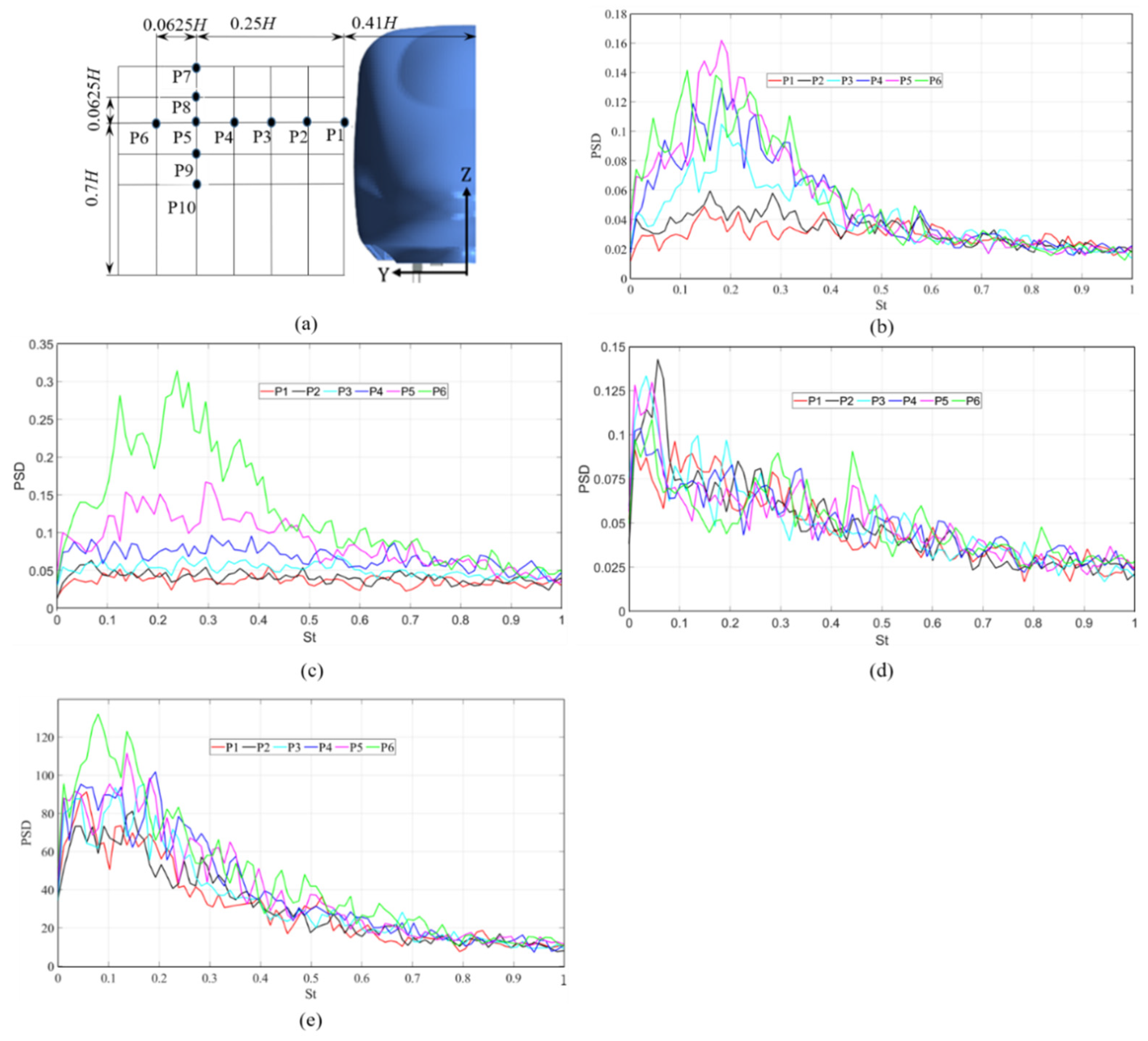
There is little literature on spanwise shedding of train leeward vortices in turbulent environments to the authors’ knowledge. Previous scholars [40,41,42] studied the tail–vehicle droop vibration of the Ahmed vehicle model. With the increase in turbulence intensity, the vibration of the train body in a crosswind environment can no longer be neglected. Figure 17 and Figure 18 show the results of the S3 plane measured by the cobra probe. The measurement points are arranged as shown in Figure 17a. The u, v and w three-way main frequencies are shown to be broadband, and the main frequency range is 0.1–0.3. P5 is the location of the vortex nucleus on the S3 surface, its v-directional vibration is the largest, and the main vibration frequency is 0.18, which is consistent with the location of the vortex nucleus in Figure 10b. Z-directional vibration at P6 is the largest, and the main frequency is 0.23.
The most dangerous conditions of the train occur at the moment of peak aerodynamic force, and the lift and side force of the head car and tail car are affected by the transient flow field, so the following studies the structure of the leeward vortex field with different nose lengths.
Q = 1 2 S 2 Ω 2 = 1 2 u ¯ i x i 2 u ¯ i u ¯ j x i x j = 1 2 u ¯ i u ¯ j x i x j
where S is the rate–strain tensor, and Ω is the rate-of-rotation tensor of the velocity variable. The iso-surfaces of positive values of Q reveal the locations in the flow where rotation dominates strain and indicate the vertical structures in the flow [35].
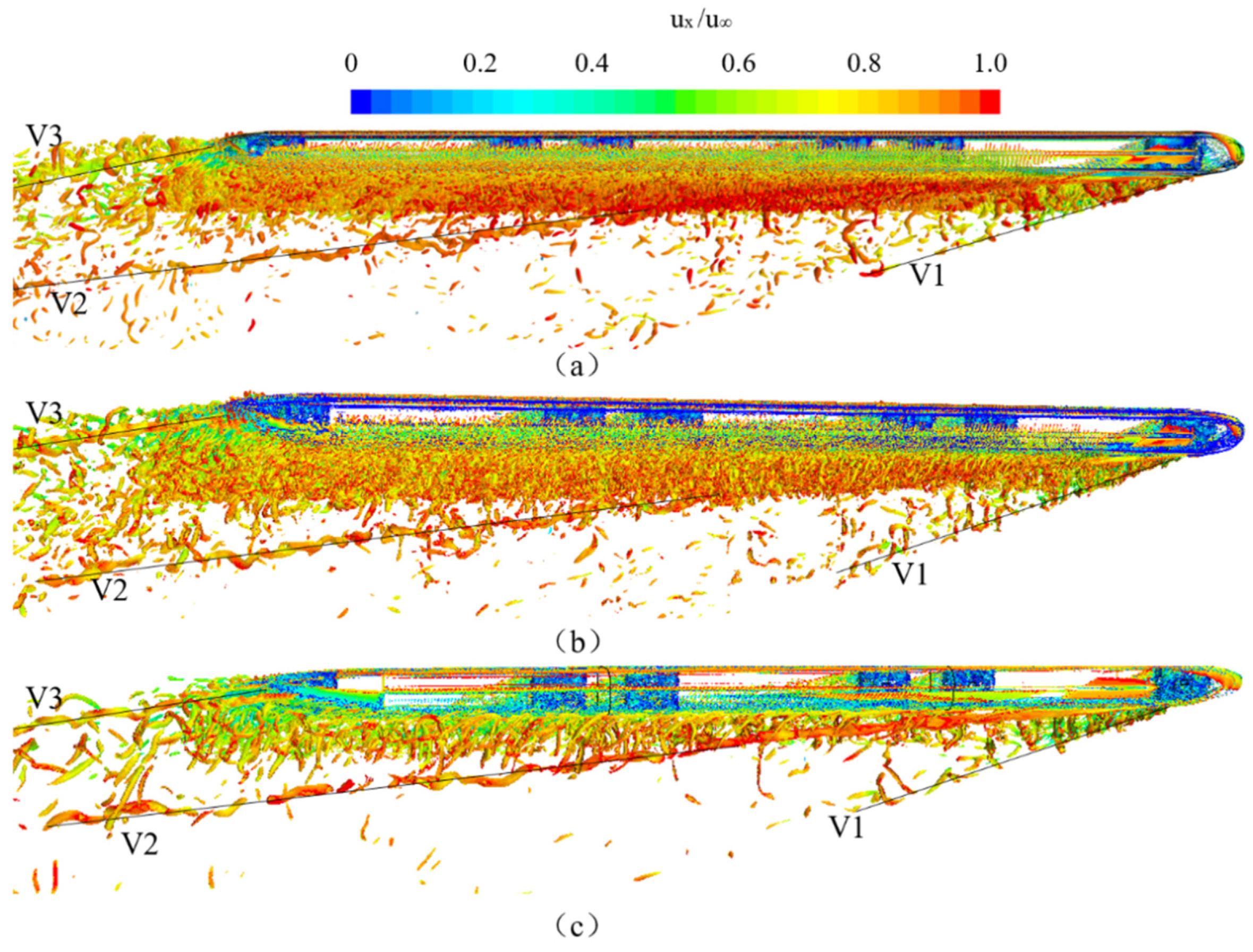
Figure 19 shows the transient flow field structure of the surrounding flow field for different train headway lengths at a 15° yaw angle, where the equivalent surface Q = 60,000, rendered using the instantaneous flow velocity.
There is a short vortex V1 at the side of the head car, which starts from the first bogie and rolls upward. The intensity of the vortex can only maintain its rotation until the first bogie of the middle car, and the angle with the flow direction becomes smaller slowly as the length of the streamlined head car increases. At the same time, the flow separation occurs when the incoming flow crosses the top of the front end and flows to the leeward side, resulting in a longitudinal vortex V2, as shown in Figure 19b,c. V2 is stronger and is maintained from the front end to the rear end, and the angle with the incoming flow is similar to V1. The longer the nose length, the smaller the angle. When the nose length is short enough, V2 beside the head car basically blends in with the leeward side and results in the breakdown of large vortices into small ones, as shown in Figure 19a. After the incoming flow passes through the tail car bogie and the gap between the body and the ground, the flow also separates on the leeward side of the tail car, forming a vortex V3, which rotates in the opposite direction of V2 and moves upward after forming at the bottom of the leeward side, and then mixes with V2 in the middle of the body. Although the V3 vortex is not as strong as V2 because it is closer to the body, it can have a stronger influence on the aerodynamic performance of the tail car leeward side.

5. Conclusions

The streamlined head and tail car shape design is the basis for the aerodynamic performance design of high-speed trains. In the present study, detailed wind tunnel experiments were used to verify the IDDES simulation results. Three nose lengths, standard and turbulent environments scenarios, and a total of six cases were used in this study to analyze the effects of head and tail lengths and inflow turbulence intensities on the aerodynamic performance of the train. The main findings are as follows:
Based on the wind tunnel experiment, the IDDES numerical simulation was proved to predict the flow structure of train leeward region correctly. The maximum difference in pressure at the same section is less than 6.7%.
When determining a high-speed train’s nose length, it must weigh between drag reduction and overturning in the crosswind. The nose length of the train cannot be extended indefinitely to reduce the drag because the overturning moment of the long tail car increases dramatically under the crosswind. Under the standard flow condition of 15° crosswind, when the streamlined nose length increases from 5m to 10m, an increase in the length of the tail car has a greater effect on the side force coefficient and the overturning moment coefficient, and the lift and overturning moment coefficients both decrease by 72.35% and 103.63%, respectively. When the nose length of the tail car becomes shorter, the vortex core of the separation flow on the leeward side of the tail car is further away from the train body under crosswind, thus delaying the flow separation on the leeward side.
At 15° yaw, increasing the turbulence intensity of incoming wind from 1% to 5% can reduce the overturning risk of the tail car. On the one hand, increasing the turbulence intensity of the incoming wind reduces the negative pressure extremum on the windward side. On the other hand, increasing the turbulence intensity of the incoming wind makes the vortex core of the separation vortex on the leeward side far away from the train body, thus achieving the effect of delayed separation. Because the vortex core on the leeward side of the head and middle cars is not fully developed, the position of the vortex cores on the leeward side of the head and middle cars is less affected.
When the airflow flows through the streamlined tail car, the pressure of the train body varies greatly for different nose lengths, and the maximum negative pressure at the tail car decreases as the streamlined length of the train increases.
The location of the time-averaged vortex core for a 15° crosswind is approximately 0.67H~0.7H high from the ground and 0.65H~0.67H wide from the center of the train. The main frequency of the leeward vortex measured by the cobra probe ranges from 0.1 to 0.3. The transient vibration amplitude at the position of the vortex core is the largest, and the main frequency of vibration is 0.18.

Author Contributions

Conceptualization, B.Y. and G.C.; methodology, X.-H.X.; formal analysis, R.-D.X.; resources, X.-H.X.; writing—original draft preparation, B.Y.; writing—review and editing, G.C.; supervision, X.-H.X.; funding acquisition, X.-H.X. All authors have read and agreed to the published version of the manuscript.

Funding

This research was funded by the National Key R & D program of China, grant number 2020YFA0710903; Transport Department of Hunan Province Technology Innovation Project, grant number 202037; Hunan Provincial Education Department Project, grant number 22B0983.

Institutional Review Board Statement

Not applicable.

Informed Consent Statement

Not applicable.

Data Availability Statement

Not applicable.

Acknowledgments

The authors acknowledge the computational resources provided by the High Performance Computing Centre of Central South University, China.

Conflicts of Interest

The authors declare no conflict of interest.

References

  1. Chen, Z.W.; Liu, T.H.; Jiang, Z.H.; Guo, Z.J.; Zhang, J. Comparative analysis of the effect of different nose lengths on train aerodynamic performance under crosswind. J. Fluids Struct. 2018, 78, 69–85. [Google Scholar] [CrossRef]
  2. Hemida, H.; Krajnović, S. LES study of the influence of the nose shape and yaw angles on flow structures around trains. J. Wind Eng. Ind. Aerodyn. 2010, 98, 34–46. [Google Scholar] [CrossRef]
  3. Baker, C.J.; Jones, J.; Lopez-Calleja, F.; Munday, J. Measurements of the crosswind forces on trains. J. Wind Eng. Ind. Aerodyn. 2004, 92, 547–563. [Google Scholar] [CrossRef]
  4. Baker, C.J. Some complex applications of the wind loading chain. J. Wind Eng. Ind. Aerodyn. 2003, 91, 1791–1811. [Google Scholar] [CrossRef]
  5. Suzuki, M.; Tanemoto, K.; Maeda, T. Aerodynamic characteristics of train/vehicles under cross winds. J. Wind Eng. Ind. Aerodyn. 2003, 91, 209–218. [Google Scholar] [CrossRef]
  6. Hoppmann, U.; Koening, S.; Tielkes, T.; Matschke, G. A short-term strong wind prediction model for railway application, design and verification. J. Wind Eng. Ind. Aerodyn. 2002, 90, 1127–1134. [Google Scholar] [CrossRef]
  7. Niu, J.Q.; Wang, Y.M.; Zhang, L.; Yuan, Y.P. Numerical analysis of aerodynamic characteristics of high-speed train with different train nose lengths. Int. J. Heat Mass Transfer 2018, 127, 188–199. [Google Scholar] [CrossRef]
  8. Sun, Z.X.; Yao, S.B.; Wei, L.; Yao, Y.; Yang, G.W. Numerical Investigation on the Influence of the Streamlined Structures of the High-Speed Train’s Nose on Aerodynamic Performances. Appl. Sci. 2021, 11, 784. [Google Scholar] [CrossRef]
  9. Chen, G.; Li, X.B.; Liu, Z.; Zhou, D.; Wang, Z.; Liang, X.F.; Krajnovic, S. Dynamic analysis of the effect of nose length on train aerodynamic performance. J. Wind Eng. Ind. Aerodyn. 2019, 184, 198–208. [Google Scholar] [CrossRef]
  10. Volpe, R.; Ferrand, V.; Silva, A.D.; Moyne, L.L. Forces and flow structures evolution on a car body in a sudden crosswind. J. Wind Eng. Ind. Aerodyn. 2014, 128, 114–125. [Google Scholar] [CrossRef] [Green Version]
  11. Baker, C.J. The flow around high speed trains. In Proceedings of the BBAA VI International Colloquium on: Bluff Bodies Aerodynamics & Applications, Milano, Italy, 20–24 July 2008. [Google Scholar]
  12. Baker, C.J.; Quinn, A.; Sima, M.; Hoefener, L.; Licciardello, R. Full-scale measurement and analysis of train slipstreams and wakes. Part 1: Ensemble averages. Proc. Inst. Mech. Eng. Part F J. Rail Rapid Transit 2014, 228, 451–467. [Google Scholar] [CrossRef]
  13. Bell, J.R.; Burton, D.; Thompson, M.; Herbst, A.; Sheridan, J. Wind tunnel analysis of the slipstream and wake of a high-speed train. J. Wind Eng. Ind. Aerodyn. 2014, 134, 122–138. [Google Scholar] [CrossRef]
  14. Bell, J.R.; Burton, D.; Thompson, M.C.; Herbst, A.H.; Sheridan, J. Moving model analysis of the slipstream and wake of a high-speed train. J. Wind Eng. Ind. Aerodyn. 2015, 136, 127–137. [Google Scholar] [CrossRef]
  15. Bell, J.R.; Burton, D.; Thompson, M.C.; Herbst, A.H.; Sheridan, J. Dynamics of trailing vortices in the wake of a generic high-speed train. J. Fluids Struct. 2016, 65, 238–256. [Google Scholar] [CrossRef]
  16. Bell, J.R.; Burton, D.; Thompson, M.C.; Herbst, A.H.; Sheridan, J. Flow topology and unsteady features of the wake of a generic high-speed train. J. Fluids Struct. 2016, 61, 168–183. [Google Scholar] [CrossRef]
  17. Bell, J.R.; Burton, D.; Thompson, M.C.; Herbst, A.H.; Sheridan, J. The effect of tail geometry on the slipstream and unsteady wake structure of high-speed trains. Exp. Therm. Fluid Sci. 2017, 83, 215–230. [Google Scholar] [CrossRef]
  18. Avadiar, T.; Bell, J.; Burton, D.; Cormaty, H.; Li, C. Analysis of High-speed Train Flow Structures Under Crosswind. J. Mech. Sci. Technol. 2016, 30, 3985–3991. [Google Scholar] [CrossRef]
  19. Raghuathan, S.; Kim, H.D.; Setoguchi, T. Aerodynamics of high-speed railway train. Prog. Aerosp. Sci. 2002, 8, 469–514. [Google Scholar]
  20. Liu, T.H.; Su, X.C.; Zhang, J.; Chen, Z.W.; Zhou, X.S. Aerodynamic performance analysis of trains on slope topography under crosswinds. J. Cent. South Univ. 2016, 23, 2419–2428. [Google Scholar] [CrossRef]
  21. Hooper, J.D.; Musgrove, A.R. Reynolds stress, mean velocity, and dynamic static pressure measurement by a four-hole pressure probe. Exp. Therm. Fluid Sci. 1997, 15, 375–383. [Google Scholar] [CrossRef]
  22. Xia, C.; Shan, X.; Yang, Z. Comparison of different ground simulation systems on the flow around a high-speed train. Proc. Inst. Mech. Eng. Part F J. Rail Rapid Transit 2017, 231, 135–147. [Google Scholar] [CrossRef]
  23. Zhang, L.; Zhang, J.Y.; Li, T.; Zhang, Y.D. Multi-objective aerodynamic optimization design of high-speed train head shape. J. Zhejiang Univ. Sci. A 2017, 18, 841–854. [Google Scholar] [CrossRef]
  24. Yang, B.; Xiong, X.H.; He, Z.; Li, X.B.; Xie, P.H.; Tang, M.Z. Feasibility of replacing the 3-coach with an 1.5-coach grouping train model in wind tunnel experiment at different yaw angles. J. Cent. South Univ. 2022, 29, 2062–2073. [Google Scholar] [CrossRef]
  25. Zhao, C.Y.; Wang, H.F.; Zeng, L.W.; Alam, M.; Zhao, X. Effects of oncoming flow turbulence on the near wake and forces of a 3D square cylinder. J. Wind Eng. Ind. Aerodyn. 2021, 214, 104674. [Google Scholar] [CrossRef]
  26. Flay, R.G.J.; Stevenson, D.C. Integral length scales in strong winds below 20 m. J. Wind Eng. Ind. Aerod. 1998, 28, 21–30. [Google Scholar] [CrossRef]
  27. Du, S.B.; Li, M.; Yang, Y. Effects of turbulence integral scales on characteristics of fluctuating wind pressure. J. Wind Eng. Ind. Aerod. 2020, 204, 104245. [Google Scholar] [CrossRef]
  28. Vita, G.; Hemida, H.; Andrianne, T. Generating atmospheric turbulence using passive grids in an expansion test section of a wind tunnel. J. Wind Eng. Ind. Aerodyn. 2018, 178, 91–104. [Google Scholar] [CrossRef]
  29. Roach, P.E. The generation of nearly isotropic turbulence by means of grids. Int. J. Heat Fluid Flow 1987, 8, 82–92. [Google Scholar] [CrossRef]
  30. Shur, M.L.; Spalart, P.R.; Strelets, M.K.; Travin, A.K. A hybrid RANS-LES approach with delayed-DES and wall-modelled LES capabilities. Int. J. Heat Fluid Flow 2008, 29, 1638–1649. [Google Scholar] [CrossRef]
  31. Ghasemian, M.; Nejat, A. Aerodynamic noise prediction of a Horizontal Axis Wind Turbine using Improved Delayed Detached Eddy Simulation and acoustic analogy. Energy Convers. Manag. 2015, 99, 210–220. [Google Scholar] [CrossRef]
  32. He, K.; Minelli, G.; Wang, J.; Gao, G.J.; Krajnovic, S. Assessment of LES, IDDES and RANS approaches of a notchback bluff body. J. Wind Eng. Ind. Aerodyn. 2021, 217, 104737. [Google Scholar] [CrossRef]
  33. Xia, C.; Wang, H.F.; Shan, X.; Yang, Z.; Li, Q. Effects of ground configurations on the slipstream and near wake of a high-speed train. J. Wind Eng. Ind. Aerodyn. 2017, 168, 177–189. [Google Scholar] [CrossRef]
  34. Chen, G.; Li, X.B.; Liang, X.F. IDDES simulation of the performance and wake dynamics of the wind turbines under different turbulent inflow conditions. Energy 2022, 238, 121772. [Google Scholar] [CrossRef]
  35. Chiu, T.W.; Squire, L.C. An experimental study of the flow over a train in a crosswind at large yaw angles up to 90°. J. Wind Eng. Ind. Aerodyn. 1992, 45, 47–74. [Google Scholar] [CrossRef]
  36. Hunt, J.; Wray, A.; Moin, P. Eddies, Stream, and Convergence Zones in Turbulent Flows; Center for Turbulent Research Report CTR-S88; Stanford University: Stanford, CA, USA, 1998. [Google Scholar]
  37. Jeong, J.; Hussain, F. On the identification of a vortex. J. Fluid Mech. 1995, 285, 69–94. [Google Scholar] [CrossRef]
  38. Chong, M.S.; Perry, A.E. A general classification of three- dimensional flow fields. Phys. Fluids A 1990, 2, 765–777. [Google Scholar] [CrossRef]
  39. Graftieaux, L.; Michard, M.; Grosjean, N. Combining piv, pod and vortex identification algorithms for the study of unsteady turbulent swirling flows. Meas. Sci. Technol. 2001, 12, 1422–1429. [Google Scholar] [CrossRef]
  40. Vino, G.; Watkins, S.; Mousley, P.; Watmuff, J.; Prasad, S. Flow structures in the near wake of the ahmed model. J. Fluids Struct. 2005, 20, 673–695. [Google Scholar] [CrossRef]
  41. Wang, X.; Zhou, Y.; Pin, Y.; Chan, T. Turbulent near wake of an ahmed vehicle model. Exp. Fluids 2013, 54, 1490. [Google Scholar] [CrossRef]
  42. Minguez, M.; Pasquetti, R.; Serre, E. High-order large-eddy simulation of flow over the ahmed body car model. Phys. Fluids 2008, 20, 095101. [Google Scholar] [CrossRef]
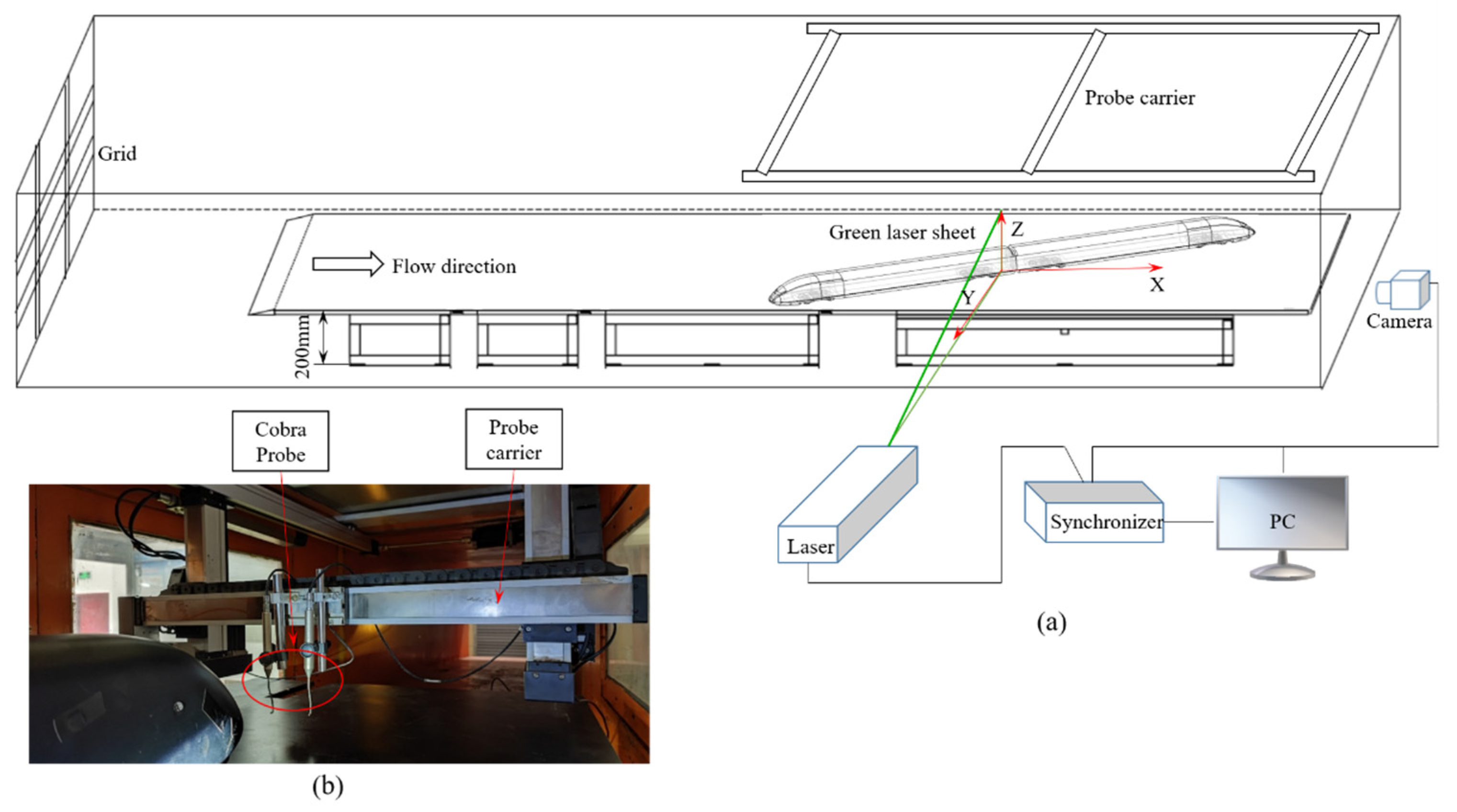
Figure 1. Schematic of experimental arrangement: (a) PIV; (b) cobra probe.
Applsci 12 12712 g001
Figure 2. Generic CRH3 model: (a) vertical projection; (b) horizontal projection.
Applsci 12 12712 g002
Figure 3. Boundary layer properties in wind tunnel: (a) velocity profile at roof of train model; (b) Ti on the roof of train model at middle position.
Applsci 12 12712 g003
Figure 4. The integral scale in wind tunnel: (a) Lx* in the x-direction; (b) Lx* in the z-direction.
Applsci 12 12712 g004
Figure 5. The computational domain: (a) boundary conditions; (b) 5 planes.
Applsci 12 12712 g005
Figure 6. The mesh of the train: (a) longitudinal cross-section; (b) lateral cross-section.
Applsci 12 12712 g006
Figure 7. Distribution of y+: (a) head car; (b) tail car.
Applsci 12 12712 g007
Figure 8. Mean aerodynamic force coefficients under smooth condition: (a) CD; (b) CS; (c) CL; (d) Cmx.
Applsci 12 12712 g008
Figure 9. Comparison of pressure at S2 plane of 5 m nose length.
Applsci 12 12712 g009
Figure 10. Time-averaged surface pressure coefficient in the five cross-sections of the train: (a) S1; (b) S2; (c) S3; (d) S4; (e) S5.
Applsci 12 12712 g010
Figure 11. Time-averaged aerodynamic force coefficient with respect to different nose lengths: (a) CD of head car; (b) CL of head car; (c) CL of tail car; (d) Cs of tail car.
Applsci 12 12712 g011
Figure 12. Velocity vector and vorticity diagram of train leeward: (a) S2 plane of Case 4; (b) S2 plane of case experimental result with 5 m train head; (c) S2 plane of Case 6; (d) S2 plane of case experimental result with 10 m head car.
Applsci 12 12712 g012
Figure 13. Streamlines and time-averaged vorticity field under 1% turbulence intensity showing the circulation regions projected onto the yz planes: (a) S1 of Case 1; (b) S3 of Case 1; (c) S5 of Case 1; (d) S1 of Case 2; (e) S3 of Case 2; (f) S5 of Case 2; (g) S1 of Case 3; (h) S3 of Case 3; (i) S5 of Case 3.
Applsci 12 12712 g013
Figure 14. Streamlines and time-averaged vorticity field under 5% turbulence intensity showing the circulation regions projected onto the yz planes: (a) S1 of Case 4; (b) S3 of Case 4; (c) S5 of Case 4; (d) S1 of Case 5; (e) S3 of Case 5; (f) S5 of Case 5; (g) S1 of Case 6; (h) S3 of Case 6; (i) S5 of Case 6.
Applsci 12 12712 g014
Figure 15. Streamlines projected on the surface of the head train: (a) Case 1; (b) Case 2; (c) Case 3; (d) Case 4; (e) Case 5; (f) Case 6.
Applsci 12 12712 g015
Figure 16. Streamlines projected on the windward side of the tail train: (a) Case 1; (b) Case 2; (c) Case 3; (d) Case 4; (e) Case 5; (f) Case 6.
Applsci 12 12712 g016
Figure 17. Spectrum analysis of horizontal measurement points near the S3 surface vortex core in wind tunnel: (a) test point arrangement; (b) v; (c) w; (d) u; (e) total pressure.
Applsci 12 12712 g017
Figure 18. Spectral analysis of the vertical points of the vortex core on the S3 surface in wind tunnel: (a) v; (b) w; (c) u; (d) total pressure.
Applsci 12 12712 g018
Figure 19. Q contours around the train with different nose lengths (Q = 60,000): (a) Case 1; (b) Case 2; (c) Case 3.
Applsci 12 12712 g019
Table 1. Spatial resolutions for 7.5 m nose length train’s three types of grids.
GridsFirst Layer Mesh ThicknessNumber of Mesh Layers in Boundary LayerBoundary Layer Grid Growth RateTotal Numbers
Coarse5.5 × 10−5 mm301.247.11 million
Medium5.0 × 10−5 mm301.270.97 million
Fine4.5 × 10−5 mm301.299.54 million
Table 2. Summary of simulations performed at a 15° yaw angle.
CaseConditionIu/(%)Lhead/(m)Total Numbersy+s+l+
1Smooth1
1
1
571.62 million0.3387.587.5
27.570.97 million0.338888
31063.31 million0.339999
4turbulence5
5
5
571.62 million0.3387.587.5
57.570.97 million0.338888
61063.31 million0.339999
Table 3. Configuration for 7.5 m nose length train’s three types of grids.
Grids C D ¯ C S ¯ C L ¯ C Mx ¯
Coarse0.12960.16250.25060.0578
Medium0.12880.16810.25720.0608
Fine0.12830.16820.25690.0597
Table 4. SDs of the overturning moment coefficient.
Case 1Case 2Case 3Case 4Case 5Case 6
Head car0.01960.01510.01560.11650.10000.0992
Middle car0.02030.02100.01970.08960.08690.0989
Tail car0.01950.01810.02430.06530.06340.0848
Publisher’s Note: MDPI stays neutral with regard to jurisdictional claims in published maps and institutional affiliations.