
Arbitrary Sampling Fourier Transform and Its Applications in Magnetic Field Forward Modeling


Abstract
1. Introduction
2. Methods
2.1. 1D AS-FT
2.2. 2D AS-FT
2.3. 3D AS-FT
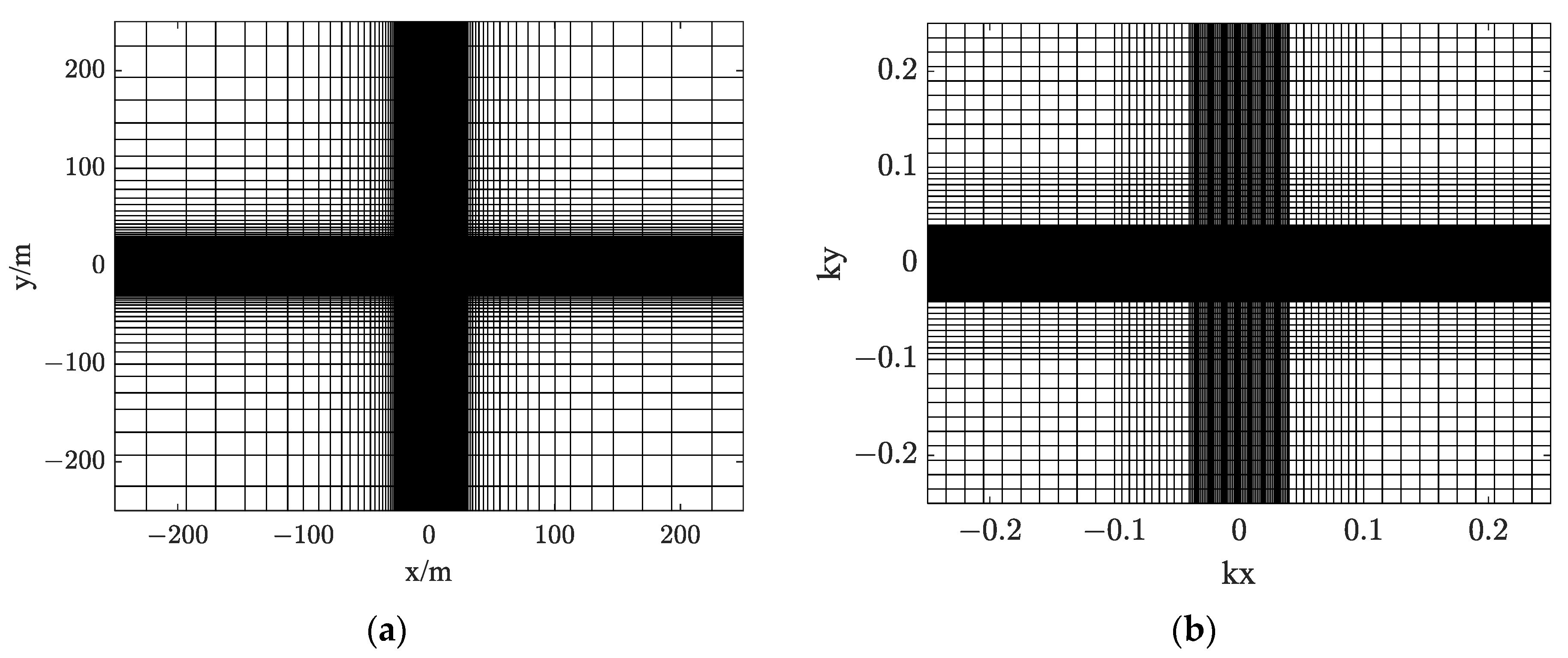
3. Sampling Rules
3.1. Forward Transform Sampling Rules
3.2. Inverse Transform Sampling Rules
4. Algorithm Analysis
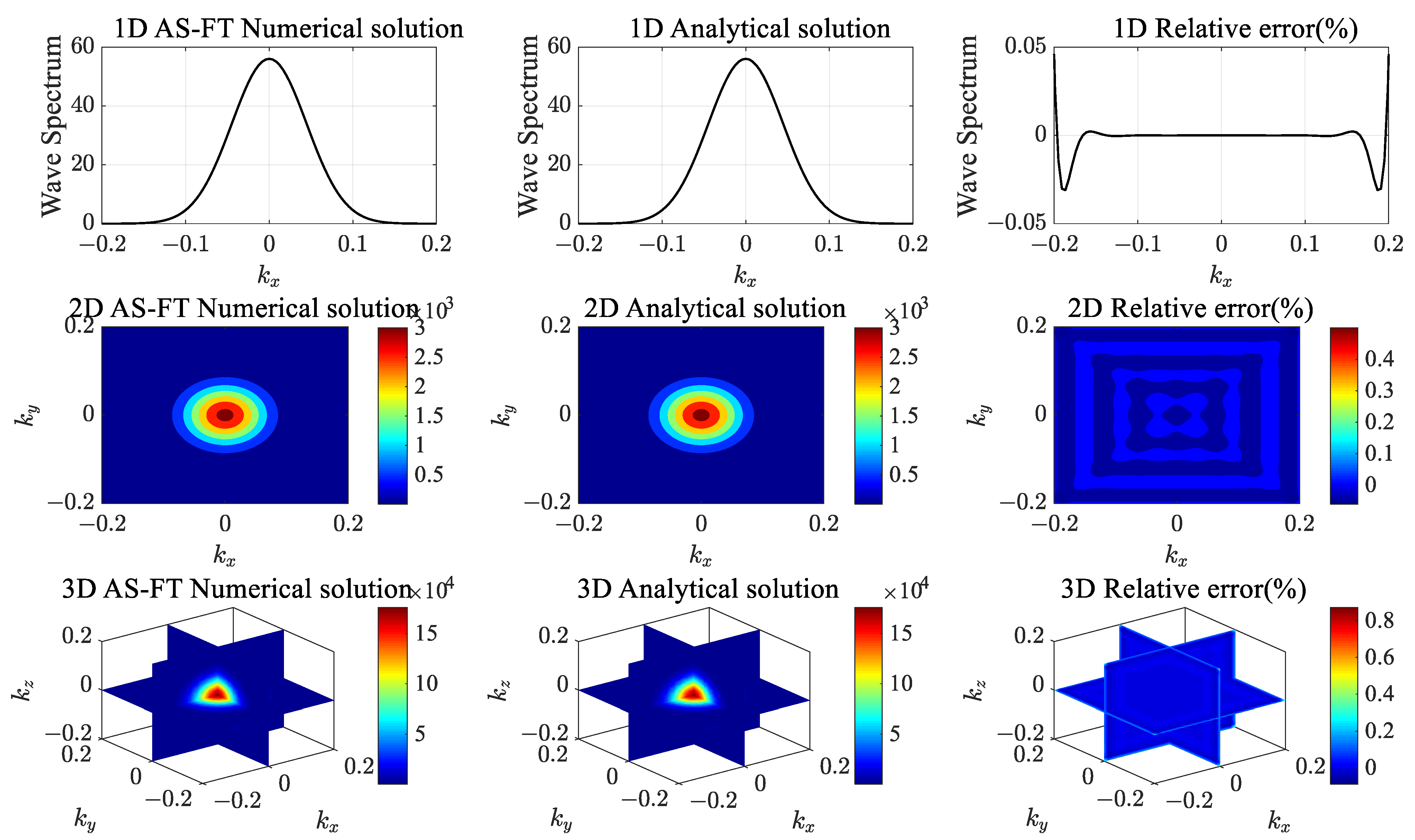
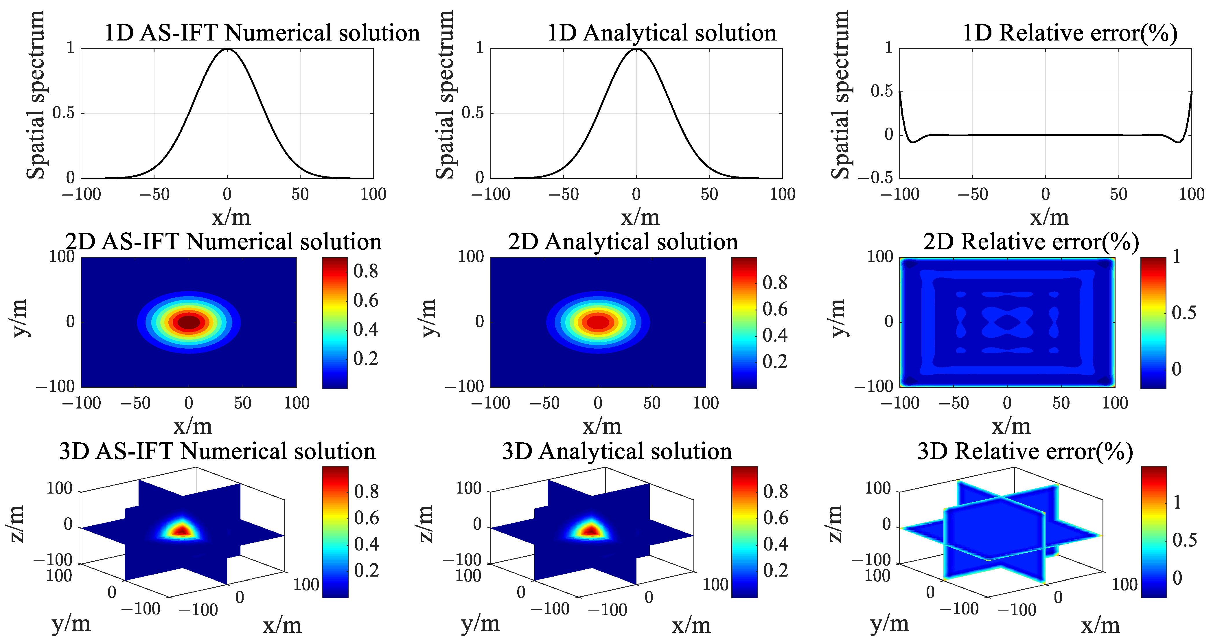
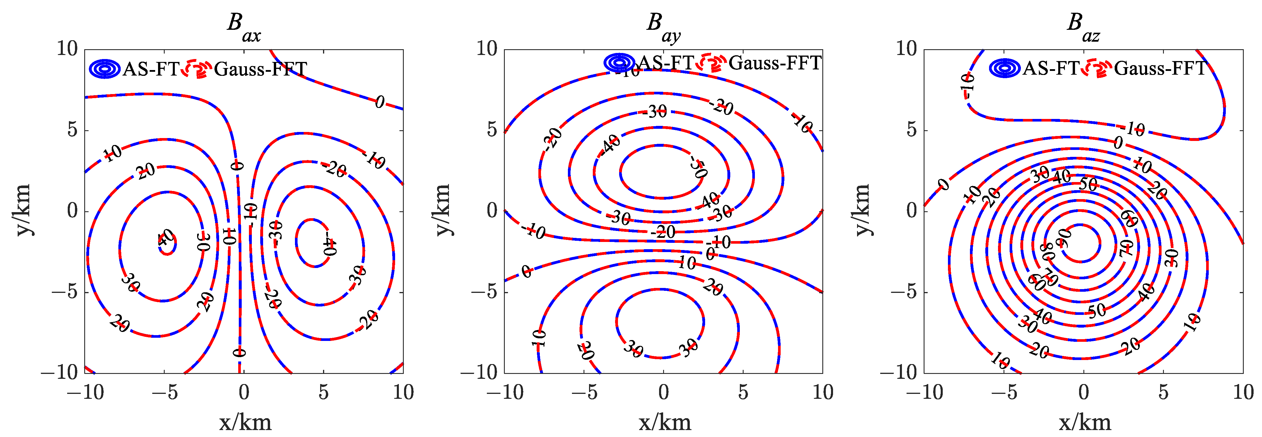
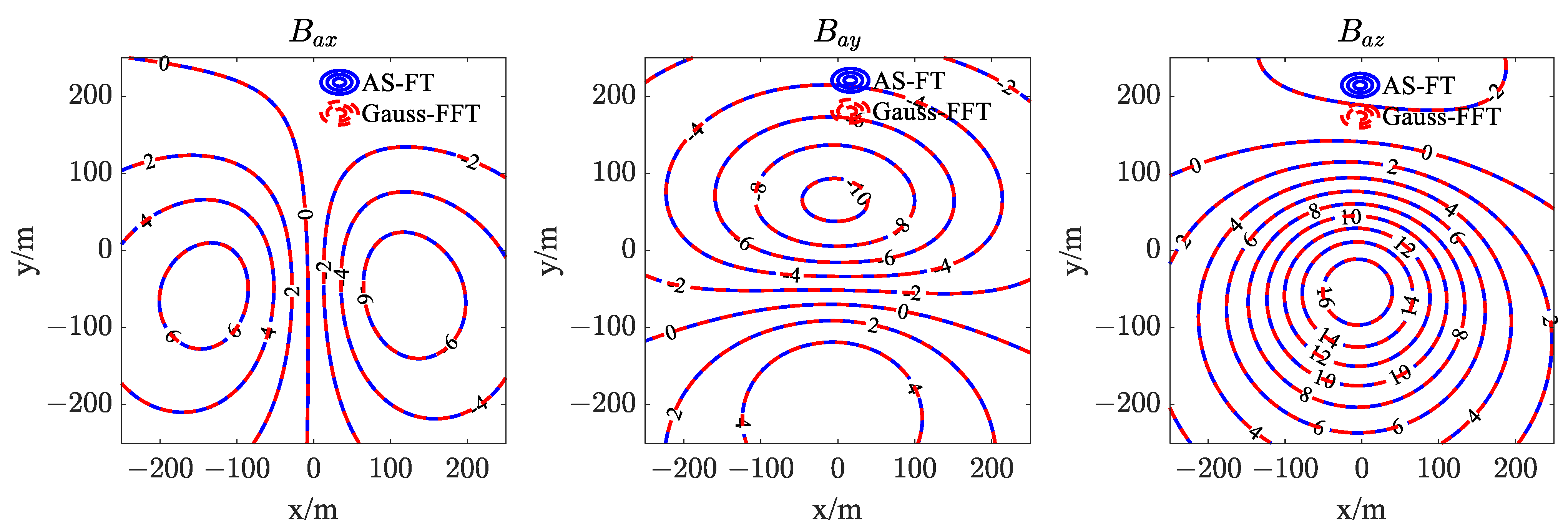
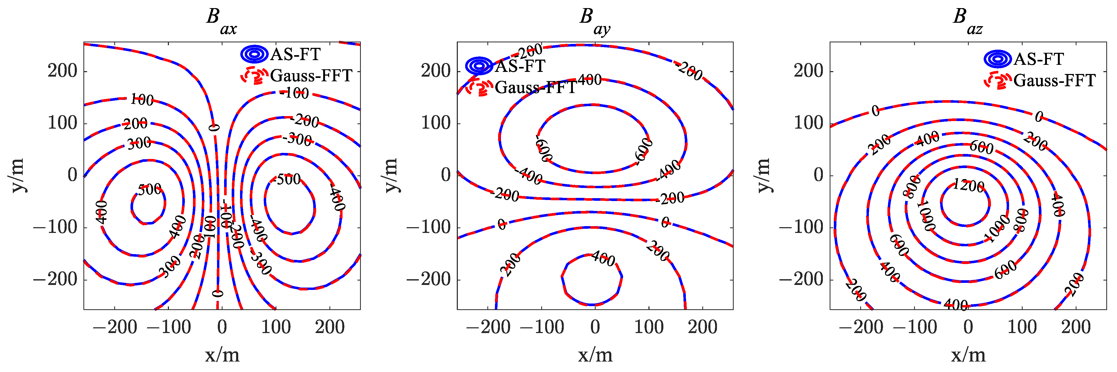
4.1. Verification of the AS-FT
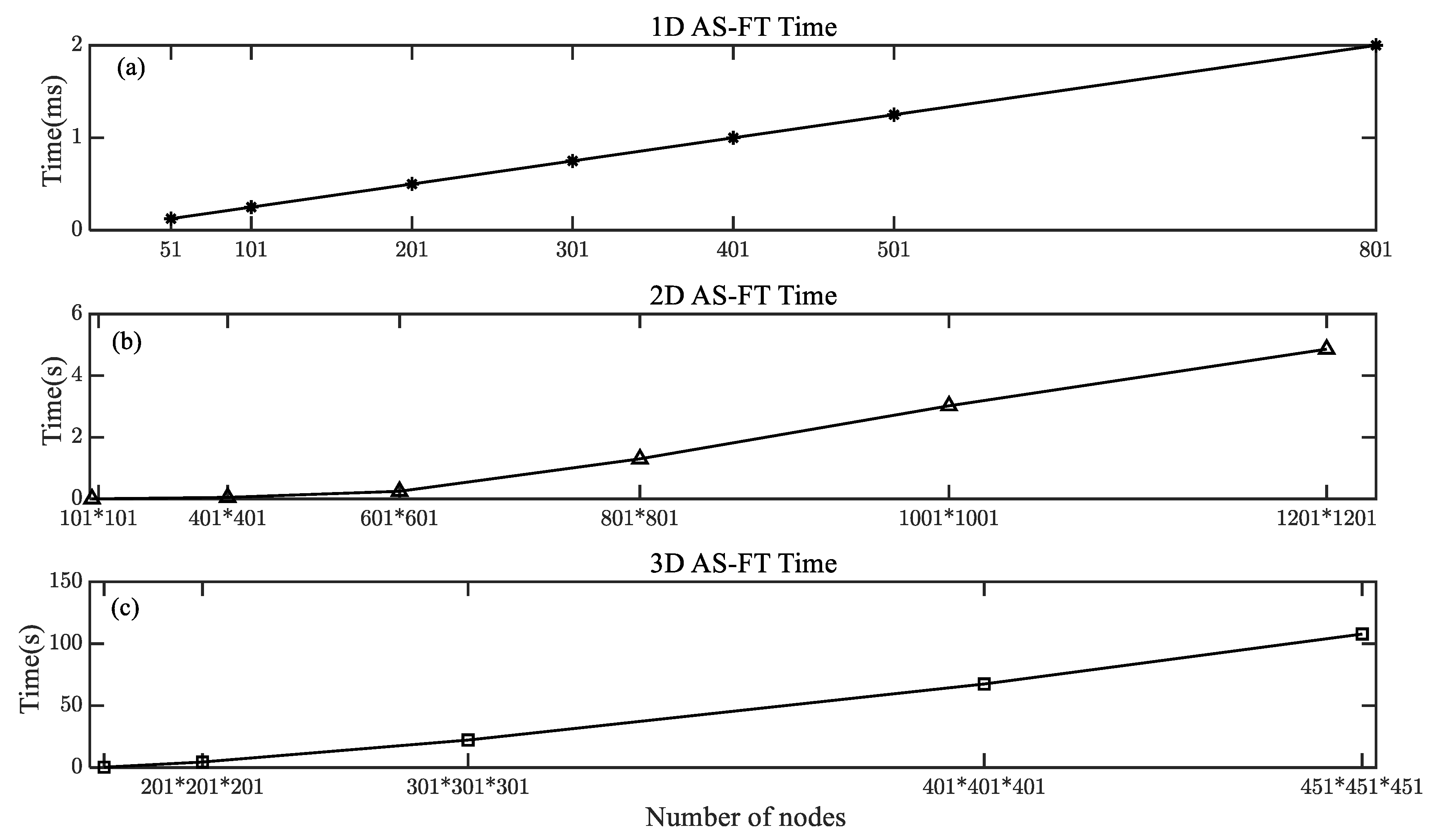
4.2. Efficiency Analysis
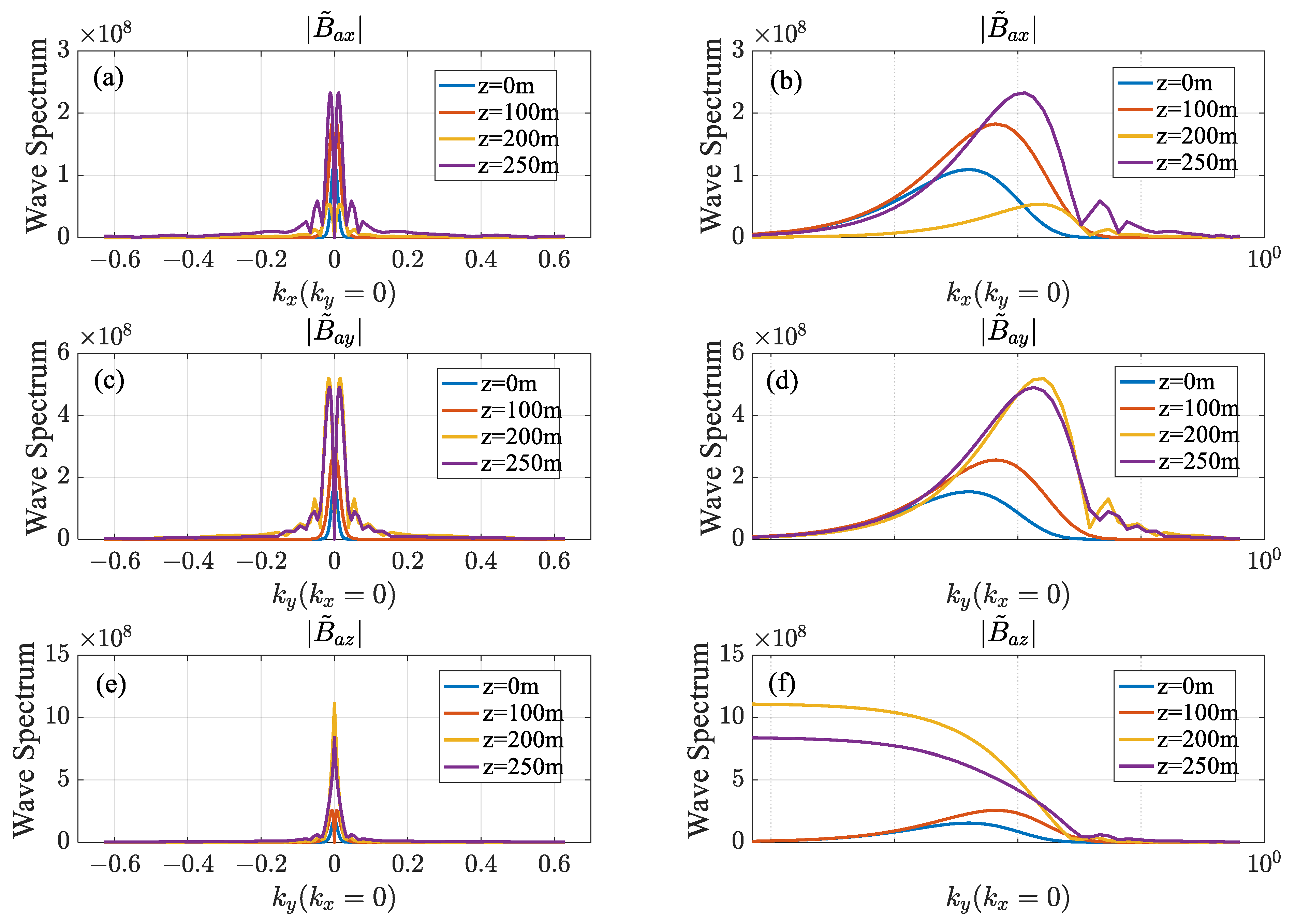
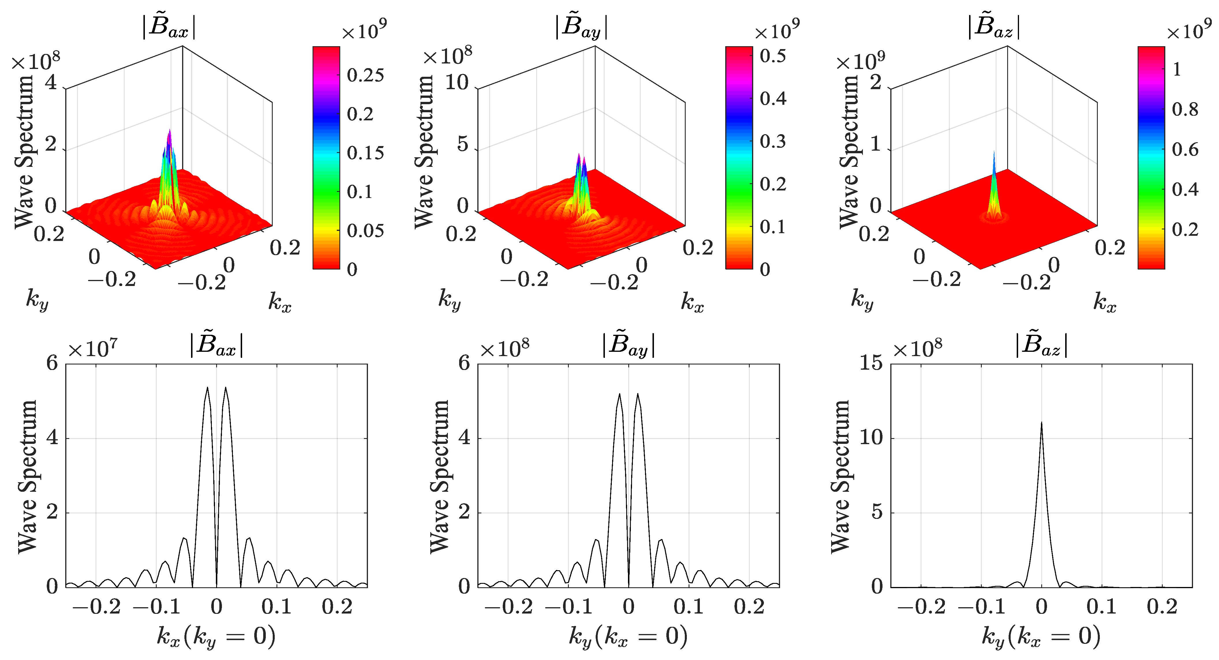
5. Results
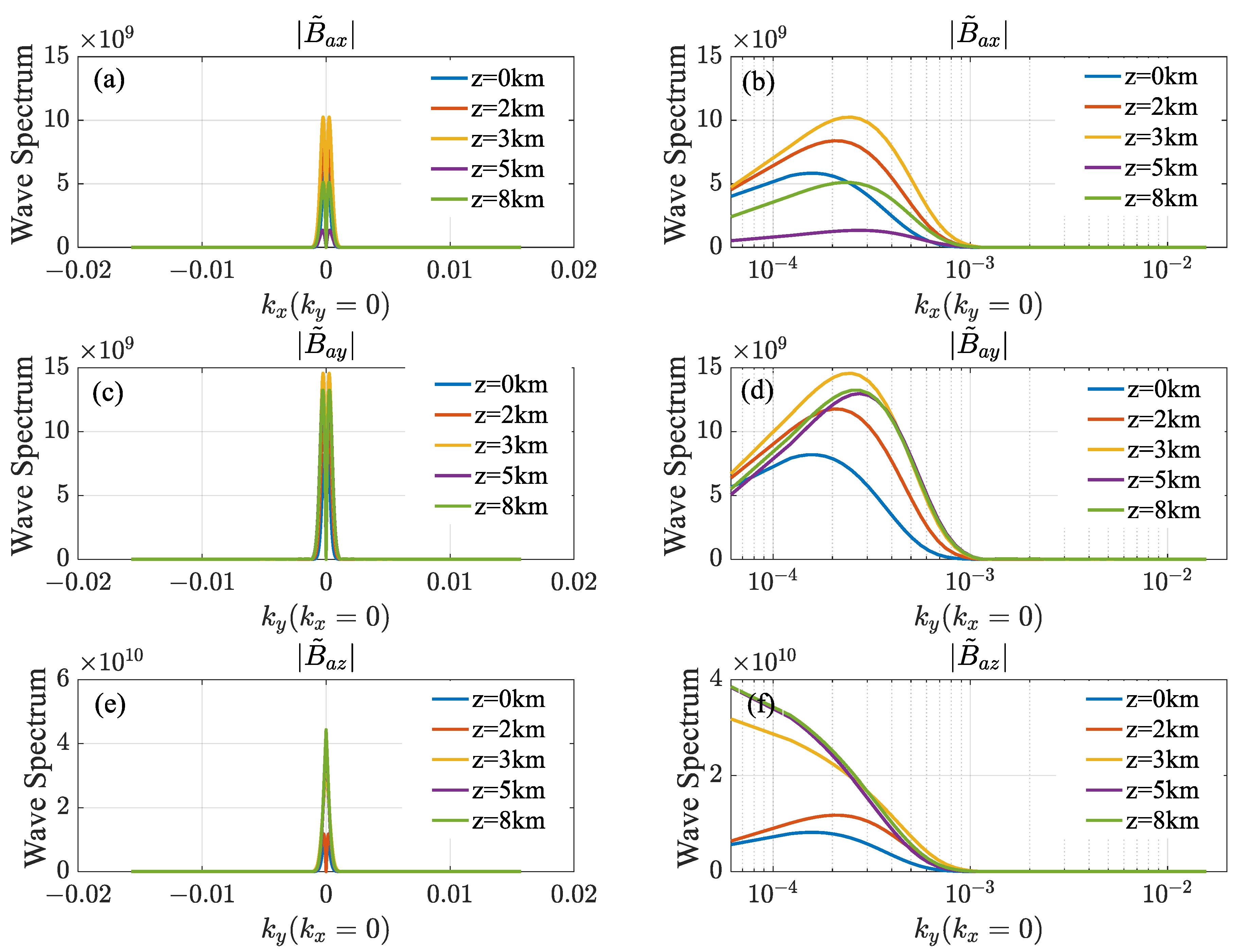
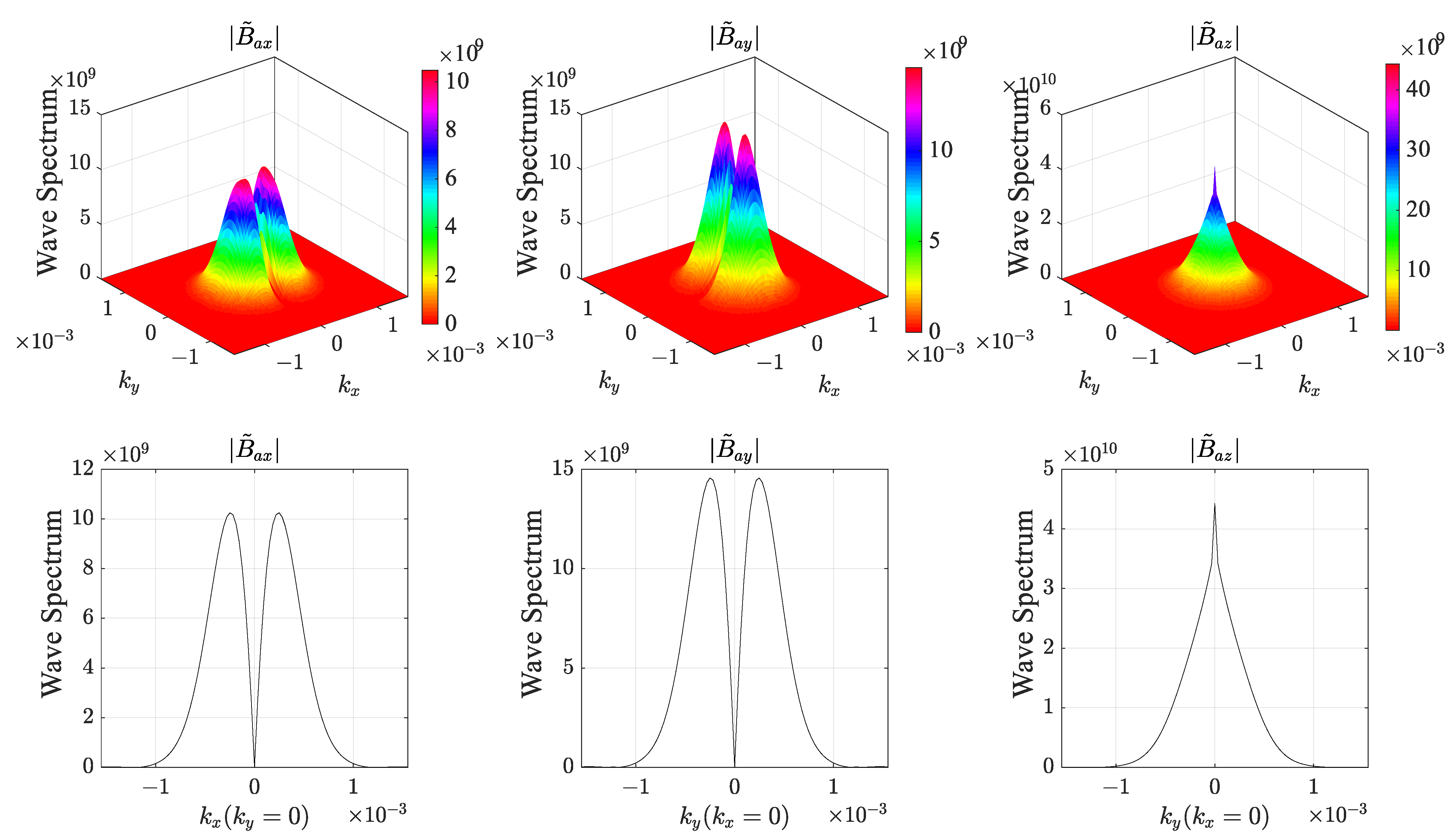
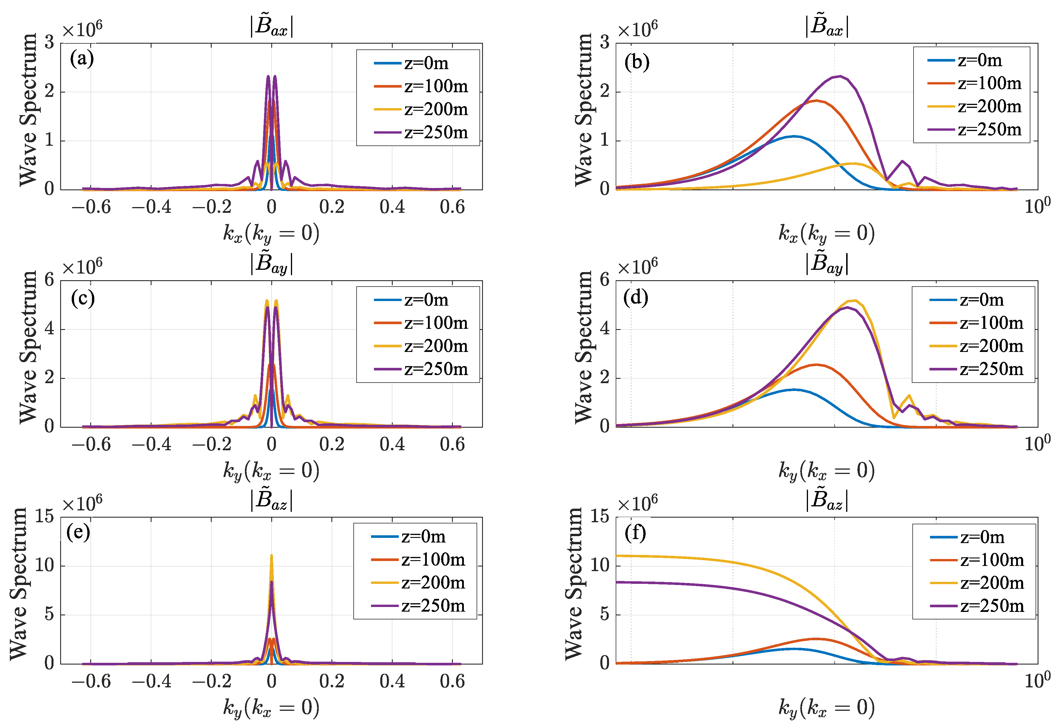
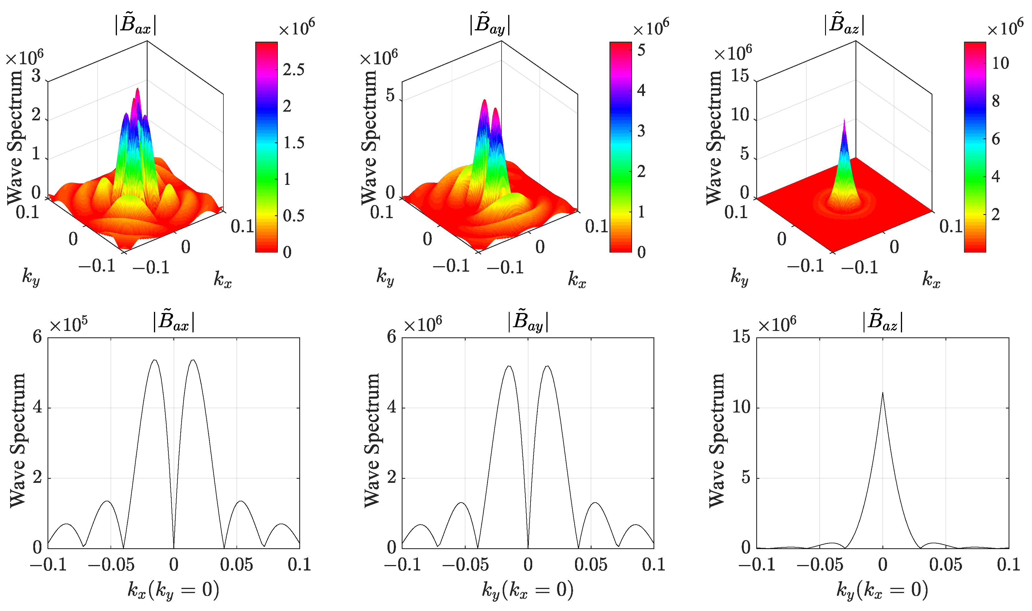
5.1. Theory of Magnetic Field Modeling in Space-Wavenumber Domain
5.2. Efficiency Comparison of Different Fourier Transform Methods
- Ke is the expansion coefficient of standard-FFT, and the expression is as follows:where S refers to the outward expansion distance from the boundary of the simulation area, and d refers to the burial depth of the abnormal body. Ke is taken as 2, 5, and 8, respectively.
- The Gauss points of Gauss-FFT are 2, 3, and 4, respectively.
- The sampling points in the spatial and wavenumber domains of AS-FT are the same and uniformly sampled.
5.3. Experiments
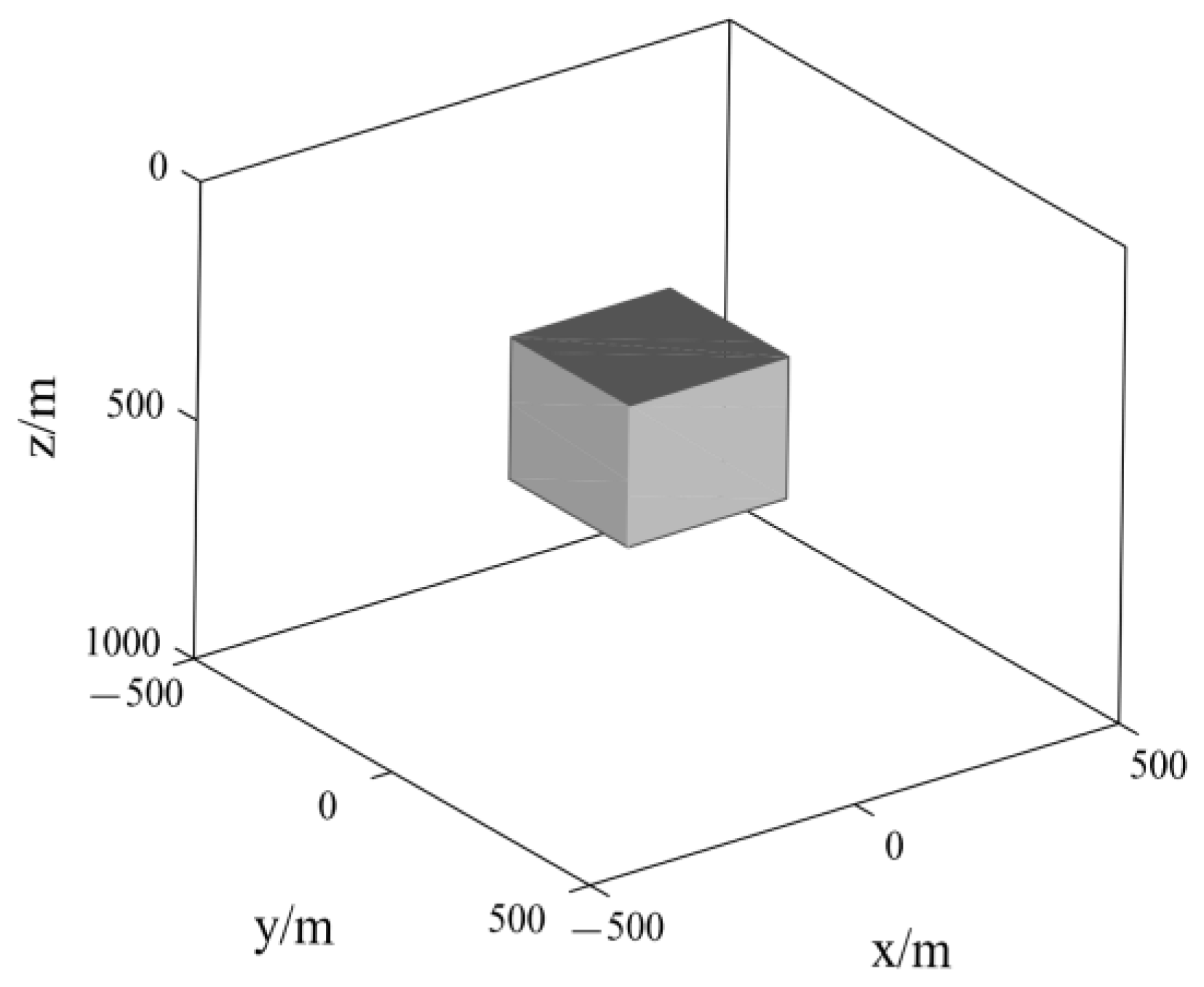
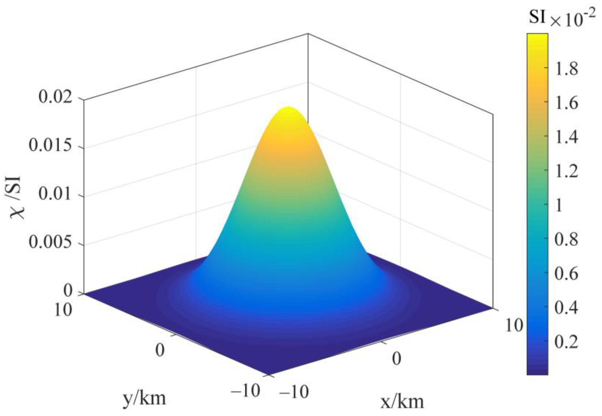
5.3.1. Weak Magnetic Continuous Medium
5.3.2. Weak Magnetic Catastrophe Medium
5.3.3. Strong Magnetic Catastrophe Medium
6. Discussion
7. Conclusions
Author Contributions
Funding
Institutional Review Board Statement
Informed Consent Statement
Data Availability Statement
Acknowledgments
Conflicts of Interest
Appendix A
References
- Bhattacharyya, B.K.; Navolio, M.E. A Fast Fourier Transform Method for Rapid Computation of Gravity and Magnetic Anomalies Due to Arbitrary Bodies*. Geophys. Prospect. 1976, 24, 633–649. [Google Scholar] [CrossRef]
- Chai, Y.P. A-E Equation of Potential Field Transformations in the Wavenumber Domain and Its Application. Appl. Geophys. 2009, 6, 205–216. [Google Scholar] [CrossRef]
- Boyd, J.P.; Marilyn, T.; Eliot, P. Chebyshev and Fourier Spectral Methods. Dover Publ. 2000, 3, 1–4. [Google Scholar] [CrossRef]
- Haskell, B. Frame-to-Frame Coding of Television Pictures Using Two-Dimensional Fourier Transforms (Corresp.). IEEE Trans. Inform. Theory 1974, 20, 119–120. [Google Scholar] [CrossRef]
- Bamberger, R.H.; Smith, M.J.T. A Filter Bank for the Directional Decomposition of Images: Theory and Design. IEEE Trans. Signal Process. 1992, 40, 882–893. [Google Scholar] [CrossRef]
- Jacquin, A.E. Image Coding Based on a Fractal Theory of Iterated Contractive Image Transformations. IEEE Trans. Image Process. A Publ. IEEE Signal Process. Soc. 1992, 1, 18–30. [Google Scholar] [CrossRef]
- Cooley, J.W.; Tukey, J.W. An Algorithm for the Machine Calculation of Complex Fourier Series. Math. Comput. 1965, 19, 297–301. [Google Scholar] [CrossRef]
- Rader, C.M. Discrete Fourier Transforms When the Number of Data Samples Is Prime. Proc. IEEE 1968, 56, 1107–1108. [Google Scholar] [CrossRef]
- Winograd, S. On Computing the Discrete Fourier Transform. Proc. Natl. Acad. Sci. USA 1976, 73, 1005–1006. [Google Scholar] [CrossRef]
- Dutt, A.; Rokhlin, V. Fast Fourier Transforms for Nonequispaced Data. SIAM J. Sci. Comput. 1993, 14, 1368–1393. [Google Scholar] [CrossRef]
- Beylkin, G. On the Fast Fourier Transform of Functions with Singularities. Appl. Comput. Harmon. Anal. 1995, 2, 363–381. [Google Scholar] [CrossRef]
- Liu, Q.H.; Nguyen, N. An Accurate Algorithm for Nonuniform Fast Fourier Transforms (NUFFT’s). IEEE Microw. Guid. Wave Lett. 1998, 8, 18–20. [Google Scholar] [CrossRef]
- Fessler, J.A.; Sutton, B.P. Nonuniform Fast Fourier Transforms Using Min-Max Interpolation. IEEE Trans. Signal Process. 2003, 51, 560–574. [Google Scholar] [CrossRef]
- Potts, D.; Steidl, G.; Nieslony, A. Fast Convolution with Radial Kernels at Nonequispaced Knots. Numer. Math. 2004, 98, 329–351. [Google Scholar] [CrossRef]
- Greengard, L.; Lee, J.Y. Accelerating the Nonuniform Fast Fourier Transform. SIAM Rev. 2004, 46, 443–454. [Google Scholar] [CrossRef]
- Frigo, M.; Johnson, S.G. The Design and Implementation of FFTW3. Proc. IEEE 2005, 93, 216–231. [Google Scholar] [CrossRef]
- Lee, J.Y.; Greengard, L. The Type 3 Nonuniform FFT and Its Applications. J. Comput. Phys. 2005, 206, 1–5. [Google Scholar] [CrossRef]
- Keiner, J.; Kunis, S.; Potts, D. Fast Summation of Radial Functions on the Sphere. Computing 2006, 78. [Google Scholar] [CrossRef]
- Keiner, J.; Kunis, S.; Potts, D. Using NFFT 3—A Software Library for Various Nonequispaced Fast Fourier Transforms. ACM Trans. Math. Softw. 2009, 36, 1–30. [Google Scholar] [CrossRef]
- Keiner, J.; Potts, D. Fast Evaluation of Quadrature Formulae on the Sphere. Math. Comp. 2008, 77, 397–419. [Google Scholar] [CrossRef]
- Barnett, A.H.; Magland, J.F.; Klinteberg, L.A. A Parallel Non-Uniform Fast Fourier Transform Library Based on an “Exponential of Semicircle” Kernel. SIAM J. Sci. Comput. 2019, 41, C479–C504. [Google Scholar] [CrossRef]
- Caratori Tontini, F.; Cocchi, L.; Carmisciano, C. Rapid 3-D Forward Model of Potential Fields with Application to the Palinuro Seamount Magnetic Anomaly (Southern Tyrrhenian Sea, Italy). J. Geophys. Res. 2009, 114, B02103. [Google Scholar] [CrossRef]
- Chai, Y.P. Shift Sampling Theory of Fourier Transform Computation. Sci. China Ser. E Technol. Sci. 1997, 40, 21–27. [Google Scholar] [CrossRef]
- Wu, L.Y.; Tian, G. High-Precision Fourier Forward Modeling of Potential Fields. Geophysics 2014, 79, G59–G68. [Google Scholar] [CrossRef]
- Wu, L. Efficient Modelling of Gravity Effects Due to Topographic Masses Using the Gauss-FFT Method. Geophys. J. Int. 2016, 205, 160–178. [Google Scholar] [CrossRef]
- Ouyang, F.; Chen, L.W. Iterative Magnetic Forward Modeling for High Susceptibility Based on Integral Equation and Gauss-Fast Fourier Transform. Geophysics 2020, 85, J1–J13. [Google Scholar] [CrossRef]
- Fan, Z.; Chen, R.S.; Chen, H.; Ding, D.Z. Weak Form Nonuniform Fast Fourier Transform Method for Solving Volume Integral Equations. Pier 2009, 89, 275–289. [Google Scholar] [CrossRef]
- Wu, L. Comparison of 3-D Fourier Forward Algorithms for Gravity Modelling of Prismatic Bodies with Polynomial Density Distribution. Geophys. J. Int. 2018, 215, 1865–1886. [Google Scholar] [CrossRef]
- Zhou, Y.M.; Dai, S.K.; Li, K. Cubic-Spline-Interpolation-Based FFT and Its Application in Forward Modeling of Gravity and Magnetic Fields. Oil Geophys. Prospect. 2020, 54, 915–922. [Google Scholar]
- Wang, X.L.; Liu, J.X.; Dai, S.K.; Guo, R.W.; Li, J.; Fan, P.Y. Fast Numerical Simulation of 2D Gravity Anomaly Based on Nonuniform Fast Fourier Transform in Mixed Space-Wavenumber Domain. J. Appl. Geophys. 2021, 194, 104465. [Google Scholar] [CrossRef]
- Ouyang, F.; Zhao, J.G.; Dai, S.K.; Chen, L.W.; Wang, S.X. Shape-Function-Based Non-Uniform Fourier Transforms for Seismic Modeling with Irregular Grids. Geophysics 2021, 86, T165–T178. [Google Scholar] [CrossRef]
- Wang, X.L.; Zhao, D.D.; Liu, J.X.; Zhang, Q.J. Efficient 2D Modeling of Magnetic Anomalies Using NUFFT in the Fourier Domain. Pure Appl. Geophys. 2022, 179, 2311–2325. [Google Scholar] [CrossRef]
- Dai, S.; Zhao, D.D.; Wang, S.G.; Xiong, B.; Zhang, Q.J.; Li, K.; Chen, L.; Chen, Q. Three-Dimensional Numerical Modeling of Gravity and Magnetic Anomaly in a Mixed Space-Wavenumber Domain. Geophysics 2019, 84, G41–G54. [Google Scholar] [CrossRef]
- Dai, S.K.; Chen, Q.R.; Li, K.; Ling, J. The Forward Modeling of 3D Gravity and Magnetic Potential Fields in Space-Wavenumber Domains Based on an Integral Method. Geophysics 2022, 87, G83–G96. [Google Scholar] [CrossRef]
- Brigham, E.O.; Morrow, R.E. The Fast Fourier Transform. IEEE Spectr. 1967, 4, 63–70. [Google Scholar] [CrossRef]
- Zienkiewicz, O.C.; Taylor, R.L.; Zhu, J.Z. The Finite Element Method: Its Basis and Fundamentals; Elsevier: Amsterdam, The Netherlands, 2005. [Google Scholar]
- Dai, S.K.; Zhao, D.D.; Zhang, Q.J.; Li, K.; Chen, Q.R.; Wang, X.L. Three-Dimensional Numerical Modeling of Gravity Anomalies Based on Poisson Equation in Space-Wavenumber Mixed Domain. Appl. Geophys. 2018, 15, 513–523. [Google Scholar] [CrossRef]
- Blakely, R.J. Potential Theory in Gravity and Magnetic Applications; Cambridge University Press: London, UK, 1996. [Google Scholar]


| Spatial Domain | Wavenumber Domain | Spatial Domain Sampling | Wavenumber Domain Sampling | |
|---|---|---|---|---|
| 1D | ||||
| 2D | ||||
| 3D |
| Methods | Nx × Ny or Nkx × Nky | N or Ke | Rrms (%) | Time (s) | ||
|---|---|---|---|---|---|---|
| Bax | Bay | Baz | ||||
| Gauss-FFT | 201 × 201 | N = 2 | 5.89 | 5.89 | 3.95 | 6.42 |
| N = 3 | 0.58 | 0.58 | 1.32 | 15.05 | ||
| N = 4 | 0.08 | 0.08 | 0.24 | 30.35 | ||
| Standard-FFT | 301 × 301 | Ke = 2 | 1.76 | 1.76 | 4.97 | 2.86 |
| 601 × 601 | Ke = 5 | 0.23 | 0.23 | 0.67 | 11.12 | |
| 901 × 901 | Ke = 8 | 0.07 | 0.07 | 0.23 | 39.51 | |
| AS-FT | 51 × 51 | / | 1.21 | 1.21 | 1.08 | 0.14 |
| 101 × 101 | / | 0.09 | 0.09 | 0.23 | 0.60 | |
| 201 × 201 | / | 0.02 | 0.02 | 0.11 | 2.53 | |
| Number of Sample | Rrms Error (%) | |||
|---|---|---|---|---|
| Spatial Domain Nx × Ny | Wavenumber Domain Nkx × Nky | Bax | Bay | Baz |
| 51 × 51 | 51 × 51 | 0.23 | 0.73 | 0.99 |
| 101 × 101 | 101 × 101 | 0.03 | 0.06 | 0.08 |
| Wavenumber Domain Sampling Methods | Rrms Error (%) | ||
|---|---|---|---|
| Bax | Bay | Baz | |
| Uniform | 0.11 | 0.17 | 0.22 |
| Log-domain uniform | 0.05 | 0.05 | 0.06 |
| Sampling Methods | Rrms Error (%) | |||
|---|---|---|---|---|
| Spatial Domain | Wavenumber Domain | Bax | Bay | Baz |
| Uniform | Uniform | 1.91 | 1.82 | 1.83 |
| Uniform | Log-domain uniform | 0.95 | 1.08 | 0.95 |
| Non-uniform | Piecewise uniform | 0.19 | 0.24 | 0.25 |
| Non-uniform | Log-domain uniform | 0.17 | 0.17 | 0.21 |
Publisher’s Note: MDPI stays neutral with regard to jurisdictional claims in published maps and institutional affiliations. |
© 2022 by the authors. Licensee MDPI, Basel, Switzerland. This article is an open access article distributed under the terms and conditions of the Creative Commons Attribution (CC BY) license (https://creativecommons.org/licenses/by/4.0/).
Share and Cite
Dai, S.; Zhang, Y.; Li, K.; Chen, Q.; Ling, J. Arbitrary Sampling Fourier Transform and Its Applications in Magnetic Field Forward Modeling. Appl. Sci. 2022, 12, 12706. https://doi.org/10.3390/app122412706
Dai S, Zhang Y, Li K, Chen Q, Ling J. Arbitrary Sampling Fourier Transform and Its Applications in Magnetic Field Forward Modeling. Applied Sciences. 2022; 12(24):12706. https://doi.org/10.3390/app122412706
Chicago/Turabian StyleDai, Shikun, Ying Zhang, Kun Li, Qingrui Chen, and Jiaxuan Ling. 2022. "Arbitrary Sampling Fourier Transform and Its Applications in Magnetic Field Forward Modeling" Applied Sciences 12, no. 24: 12706. https://doi.org/10.3390/app122412706
APA StyleDai, S., Zhang, Y., Li, K., Chen, Q., & Ling, J. (2022). Arbitrary Sampling Fourier Transform and Its Applications in Magnetic Field Forward Modeling. Applied Sciences, 12(24), 12706. https://doi.org/10.3390/app122412706