Three-Dimensional Hydrodynamic Analysis of a Flexible Caudal Fin

Abstract

A 3D fluid–structure coupled simulation of a square flexible flapper, the basic model of a caudal fin, is performed to visualize the flow field around the caudal fin. A plate immersed in a water tank is driven to oscillate vertically by its leading edge. A quantitative analysis of the thrust generated by the plate, which is difficult to explore experimentally, is performed over a range of non-dimensional flapping frequencies 0.93 $<f^{*}<$ 1.47 to explore the mechanism of thrust generation in more detail. Comparisons are made between three different flapping frequencies around the structural resonance. Numerical results at different flapping frequencies provide a reasonable estimate of the trailing edge amplitude and phase lag of the motion of the plate’s leading and trailing edges. The pressure distribution and deformation of the plate are analyzed to estimate the time evolution of the maximum and minimum thrust generation during the flapping period. Variations in pressure distribution on the plate surface are mainly due to the displacement of the trailing edge relative to the leading edge. Thrust is mainly provided by the pressure difference at the trailing edge. The maximum thrust was found to correspond to the maximum relative deformation of the trailing edge. The optimum frequency $f^{*}$ = 1.2 corresponding to the maximum thrust generation does not coincide with the structural resonance frequency, but remains at a frequency slightly higher than the resonance. These results indicate that the relative deformation of the plate plays an important role in the estimation of the flow field and the associated thrust generation. The numerical results may provide new guidelines for the design of robotic underwater vehicles.

1. Introduction

Aquatic animals and insects propel themselves through the surrounding liquid by flapping their flexible fins and wings. Many studies have focused on propulsion mechanisms with rigid or soft flappers. As a means of realizing how thrust forces are generated and better swimming performance is achieved, some recent studies use bionic robotic models of fish caudal fin [1,2,3,4,5], rigid flat plate [6], flexible fins [7] and insects in forward flight; cicada [8] and butterfly [9]. Propulsion mechanisms of aquatic animals corresponding to structural resonance have also been investigated experimentally and numerically in recent studies [10,11,12,13,14,15,16,17,18]. These aforementioned studies clearly show that the flexible panels, which operate at or near a resonant frequency, always achieve the optimal condition.

Experiments on a flexible rectangular plate in a uniform water flow by Florine Paraz et al. [10] reported that the optimum frequency for maximum thrust is achieved by tuning the actuating frequency of the flexible foil to the resonance of the system. Kato [11] also conducted an experimental study on the heaving motion of rectangular flat plates in water and reported a significant relationship between the flow pattern induced by the plates and the flapping frequency that causes the plates to oscillate. It was observed that the fluid motion induced by a heaving elastic plate was governed by the structural resonance of an elastic plate and its deformation. An experimental investigation on the propulsive performance of a heaving flexible panel showed that the time-averaged net thrust experiences localized boosts near resonant frequencies where the trailing edge amplitude is maximized [12]. Leftwich et al. [13] experimentally investigated the influence of passive tail flexibility on thrust production using a robotic lamprey. They reported that the force production could be increased when the cycle frequency was changed to the resonant frequency of the tail. A freely moving wing with active heaving in a fluid was studied experimentally and numerically by Spagnolie et al. [14]. They showed that the horizontal velocity was largest when the flapping frequency was near the immersed system’s resonant frequency.

The computations of Hoover et al. [15] presented the role of resonance in swimming performance by using a three-dimensional flexible panel heaving sinusoidally at its leading edge. This study showed that the local peaks in the normalized trailing edge amplitude achieved by the panel coincide with the local peaks in forward swimming speed. The work of Michelin et al. [16] focused on a simplified two-dimensional propulsion problem using a flexible wing of infinite span, actuated at its leading edge in a purely heaving motion. Their results indicated that the resonant frequency could induce maximum values of the mean developed thrust and power input. In the analytical work of [17], the propulsive performances were investigated using a two-dimensional foil with pitching and heaving motions about arbitrary pivot points. Their results also indicated that the local maxima in the amplitude of the flexural component of the deflection roughly correspond to local maxima in thrust and in power coefficients.

However, results from other studies in self-propelled conditions [19,20,21] reported that the optimal flapping frequency for the maximum cruising velocity and maximum propulsive efficiency appeared at a frequency below the resonance. Ramananarivo et al. [19] conducted an experimental investigation on the performance of flapping flyers with a self-propelled simplified insect model in air. Their results indicated that maximum performance was obtained at a frequency lower than the resonance. This observation coincides with the results reported by Thiria et al. [20] for a self-propelled model of flexible wing flapping in air, in which the optimum flapping frequency for the propulsive efficiency occurs below the natural relaxation frequency. Numerical simulation of a self-propelled plunging foil was conducted by Zhu et al. [21] to investigate the hydrodynamic effect of passive flexibility. They showed that the optimum performance is always achieved at a forcing frequency much lower than the resonance point. On the other hand, Masoud et al. [22] studied numerically the thrust generation of a fixed flexible body in air and reported that the propulsive efficiency reached a maximum at a certain flapping frequency above the resonant frequency. Dewey’s experiments [23] on a flexible panel oscillating in water with different elastic modulus showed that the structural resonance could not contribute to the efficient locomotion of flexible propulsors. This efficient locomotion was predicted to occur by considering both the optimum Strouhal number and structural resonant frequency. In the experimental work of Gibouin et al. [24], it was found that the thrust developed by the flexible robotic fish depend on the amplitude of tail and oscillation frequency, irrespective of whether the oscillation frequency is resonance or not. On the other hand, the mechanism of thrust generation in flapping-type propulsion is still a matter of debate.

Baba [25] experimentally investigated the flow field around the caudal fin using an elastically deformable flat plate that simulates the self-propelled motion of aquatic organisms. As a representation of geometric shape, the three types of caudal fin with different trailing edges and different aspect ratios were selected and the velocity field measurements by PIV were performed at different forcing frequencies around the resonance. It was observed that the average velocity distribution of the caudal fin induced a jet-like flow in the wake of the caudal fin, which shows the generation of thrust. For the maximum value of thrust production, it was confirmed that the flapping frequency remains in the higher frequency region and did not match the structural resonant frequency. Motivated by the earlier observations, we extend the experimental work of Baba et al. on a basic model of square-shaped flat plate in a flapping motion using three-dimensional numerical simulation for the fluid structure interaction of a flexible plate [25]. In the experimental work by [1], the authors reported that even using simple flexible foils and actuation only in heave, complex wake flows can be generated that strongly resemble fish locomotor wake patterns. A square flat plate is desirable as it allows the complex fluid structure interaction problems to be investigated. For solving the fixed and flexible boundaries, the coupled fluid structure interaction methods, which provide mathematically and computationally efficient algorithms, have been recently presented by some authors [26,27]. In the current study, simulations are conducted with a solver provided in open-source CFD software OpenFOAM. The objective of this study is to ascertain the reliability and accuracy of the current methodology in three-dimensional analysis of fluid structure interaction of a square-shaped flexible plate. A quantitative analysis of thrust force generated by the plate, which is experimentally difficult to explore, is performed over a range of flapping frequencies. The mechanism of thrust generation is explained by analyzing the pressure distributions around the flapping plate and the relative deformation of trailing edge. Comparisons are made between the three different flapping frequencies present around the structural resonance to gain insight into the mechanism of the associated thrust generation.

2. Materials and Methods

A three-dimensional numerical simulation of fluid flow around a flapping plate is conducted using a partitioned solver fsiFoam, which is implemented in an open-source CFD software OpenFOAM with a version of foam-extend-3.2. In this solver, the force and displacement are calculated from the fluid and solid fields and coupled at the fluid structure interface using the Dirichlet–Neumann procedure. A strongly coupled procedure is used to enforce the equilibrium of the force and displacement on the interface in each time step [28]. This solver uses the algorithm of Pressure Implicit with Split Operators (PISO) for the coupling of velocity and pressure. The temporal term is discretized by the first-order implicit Euler method with the time step of 0.005 s. The spatial discretization is performed with the second-order schemes: Gauss linear for gradient and divergence terms, and Gauss linear skewCorrected for Laplacian terms. The generalized geometric-algebraic multi-grid (GAMG) algorithm and pre-conditioned bi-stab conjugate Gradient (PBiCG) algorithm are applied for solving the linear system of pressure and velocity equation. More details about the governing equations for fluid and solid fields can be seen in reference [29].

2.1. Geometric Model

Figure 1 shows the schematic geometry of a square flexible flat plate, which has the same dimensions and size as that in the experiments of Baba et al. [25]. The flat plate has the dimensions of root length, $L_r$ = 40 mm, chord length, $L_c$ = 40 mm and uniform thickness of 1 mm. The flapping motion is imposed to the leading edge of the plate in a stationary fluid. The leading edge of the plate is set to vibrate vertically in the z direction and its displacement is described as follows:

$$z_r=A_{r}sin\left(2\pi \varphi \right),\varphi =ft(0<\varphi <1),$$

(1)

where $z_r$ denotes the z position of the leading edge of the plate, $A_r$ is the flapping amplitude and $\varphi$ is the non-dimensional phase. The terms f and t represent the flapping frequency and time, respectively. The flapping frequency is normalized by the natural frequency of the plate to obtain the non-dimensional frequency of $f^{*}$. The flapping amplitude is kept constant at 3 mm under different non-dimensional frequencies of $f^{*}$. The plate is made of silicone material that has a modulus of elasticity of 5.6 MPa. The simulations are carried out in a stationary fluid with a density of $\rho =1.0\times {10}^3$ kg/m${}^3$ and kinematic viscosity of $\nu =1.0\times {10}^{-6}$ m${}^2$/s.

2.2. Computational Domain and Boundary Conditions

To reduce computational burden, only half of the fluid and solid domain is considered and a symmetry plane is placed at the center of leading edge along the x-direction. Only half of the 40 cm span length of the plate (i.e., 20 cm for half of the plate) is simulated. The computational domain extends 7 mm and 145 mm in the positive and negative x-direction from the leading edge, 60 mm in the y-direction from the symmetry plane of the plate, and 75 mm above and below the plate in the z-direction. These boundaries are within the range of boundaries in the experimental tank and large enough to have negligible effects on the moving plate. The computational domain with a square-shaped flat plate as a schematic view is shown in Figure 2, with x, y and z denoting the direction of thrust, span of the plate and normal to the plane of the plate, respectively. The number of hexahedral cells in the fluid and solid domains are about 237, 860 and 1400. Computations are conducted on a PC equipped with an Intel^® Core™ i5-5257U CPU 2.70 GHz × 4 processor and it took about 22 h for the calculation of seven flapping cycles in the lower frequency range.

The symmetryPlane boundary condition is used for the front planes of the fluid and solid domains. The $\mathit{movingWallVelocity}$ and $\mathit{zeroGradient}$ boundary conditions are specified to both the velocity and pressure on the patch named as $\mathit{interface}$, which is coupled with the plate surface. For the boundary condition on the side, top and bottom patches, the $\mathit{totalPressure}$ and $\mathit{zeroGradient}$ are defined for the pressure and velocity, respectively. For the solid domain, the imposed flapping motion is applied to the leading edge of the plate and the boundary condition on the interface of the plate surface is utilized with $\mathit{tractionDisplacement}$ for the displacement.

3. Results

3.1. Validation and Grid Independence Study

To validate the $\mathit{fsiFoam}$ solver used in this paper, the motion of the plate is simulated for different non-dimensional frequencies $f^{*}$ and compared with the experimental results of Baba et al. [25]. The results are compared in terms of trailing edge amplitude and phase lag between the leading and trailing edge motion. The motion of the plate’s trailing edge can be expressed by its vertical displacement $z_t$ as;

$$z_t=A_{t}sin\left(2\pi {\varphi }_t\right),{\varphi }_t=\varphi -{\varphi }_{\mathrm{lag}},$$

(2)

where ${\varphi }_{\mathrm{lag}}$ is a phase lag between the motion of trailing edge and leading edge of the plate and $A_t$ is the amplitude of trailing edge’s motion.

Simulations are conducted for the non-dimensional frequency in the range of 0.93 $<f^{*}<$ 1.47, which is around the range of resonant frequency. The three flapping frequencies with the increment of 0.4 Hz, f = 1.4, 1.8 and 2.2 Hz, are selected for this non-dimensional frequency range and the amplitude of motion $A_r$ = 3 mm is kept constant for all cases. The computed trailing edge amplitudes $A_t$ and phase lags are compared with the corresponding experimental data as shown in Figure 3. A reasonable agreement is observed in the trend of amplitude and phase lag despite some discrepancies in the magnitude. The resonance frequency of this plate is observed to be $f_n$ = 1.5 Hz, which is close to the value of $f_n$ obtained in the experiments of Baba et al. [25]. The experimental and numerical results are also presented in

Table 1. Results of trailing edge amplitude $A_t$.

${\mathit{f}}^{*}$	Experiment	Simulation
0.93	6.54 mm	6.62 mm
1.20	5.88 mm	5.96 mm
1.47	4.98 mm	5.10 mm

and

Table 2. Results of phase lag ${\varphi }_{\mathrm{lag}}$.

${\mathit{f}}^{*}$	Experiment	Simulation
0.93	0.456 × $\pi$ rad	0.440 × $\pi$ rad
1.20	0.630 × $\pi$ rad	0.620 × $\pi$ rad
1.47	0.750 × $\pi$ rad	0.716 × $\pi$ rad

.

In order to conduct a grid independence study, the calculations are performed for three different resolutions of the computational mesh in the fluid domain; coarse mesh, medium mesh and fine mesh. The coarse mesh contains 118,744 cells, the medium mesh contains 237,860 cells and the fine mesh contains 475,880 cells. The solid domain contains 1400 elements uniformly distributed. The test case is based on the flapping frequency of f = 1.4 Hz. The effects of mesh resolution on the displacement of trailing edge are shown in Figure 4. The results show that the difference in the peak value of trailing edge displacement is about 2.65% between the medium and fine mesh. Therefore, the medium mesh is adopted for all simulations in the present study.

3.2. Hydrodynamic Analysis

3.2.1. Thrust Production

The thrust force is simply a force that advances toward the flow as a component force induced by the deformation of the plate. The thrust force, $F_T$, in the x-direction is computed as $F_T$ = 0.5 $C_T{U}^2\rho a$, where $C_T$ is the thrust coefficient, U is the maximum translational velocity of model fin, $\rho$ is the fluid density and a is the reference area of the plate. The mean thrust shown can be obtained by averaging the instantaneous thrust values over the entire flapping cycle.

In the corresponding experiments, the thrust force was calculated from the momentum integration theorem. The plate did not move while it was vibrated in the z-direction and the velocity fields around the flapping plate were measured by PIV [25]. In the present study, the thrust force $F_T$ and thrust coefficients $C_T$ are calculated using a post-processing function tool available in OpenFOAM.

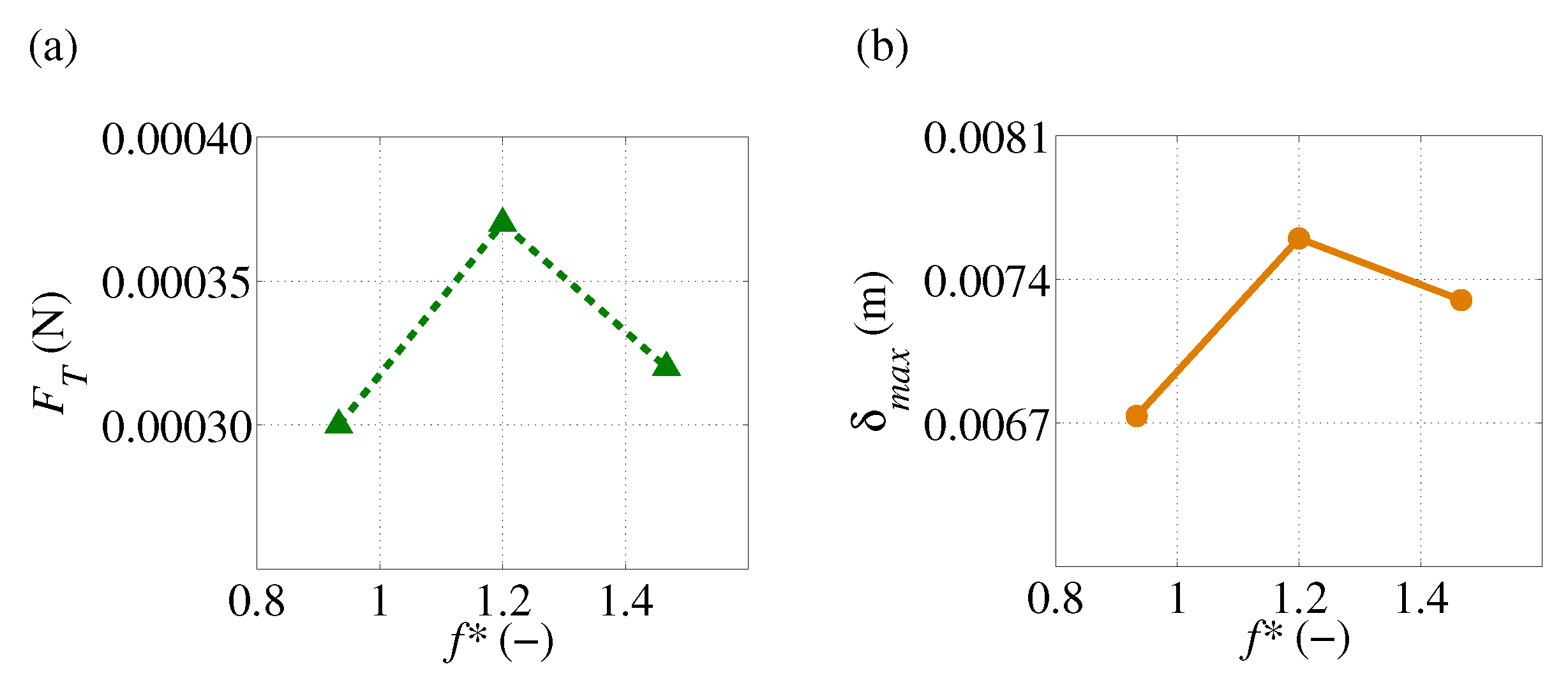
Figure 5a shows the variation of mean thrust force with different $f^{*}$, which can be used to reveal the effect of $f^{*}$ on the propulsive characteristics more clearly and quantitatively. It illustrates that the thrust gradually increases with $f^{*}$. Thrust increases with $f^{*}$ and reaches a maximum at a certain value of $f^{*}$. However, after reaching a certain value of $f^{*}$, the mean thrust of the plate decreases gradually. This presents an indication that there is an optimal value of $f^{*}$ at which the plate achieves the highest mean thrust. For the frequency range considered in our simulations, it is observed that the maximum net thrust occurs at $f^{*}$ = 1.2 and the corresponding phase lag is observed to be 0.62$\pi$ radians. The trend of variation in thrust is observed to be consistent with that in [25].

In this situation, the magnitude of trailing edge amplitude seems to be irrelevant to the generation of maximum thrust force since it decrease monotonically with flapping frequency as shown in Figure 3a. It would seem that the generation of maximum thrust force comes from the phase lag due to deformation, which makes a difference in the displacement of the trailing edge relative to the displacement of leading edge. Figure 5b shows the maximum deformation of the trailing edge relative to the leading edge for all cases. Note that the instantaneous displacement of leading edge $z_r$ is subtracted from that of trailing edge $z_t$ to obtain the instantaneous relative displacement of the trailing edge in a flapping cycle, $z_t-z_r$, from which the maximum relative deformation of trailing edge, ${\delta }_{max}$, is estimated. This means that the amplitude of the instantaneous relative displacement of trailing edge in a flapping cycle is taken as the maximum relative deformation of trailing edge ${\delta }_{max}$.

According to Figure 5a,b, the maximum net thrust is found to be associated with the maximum value in the relative deformation of trailing edge. It is evident that the phase lag is due to deformation of the plate, which makes a difference in the relative deformation of the trailing edge with respect to the leading edge, influences the generation of thrust force. Notably, the optimal value of $f^{*}$ for maximum thrust generation in this plate does not coincide with the optimal value of $f^{*}$ for the elastic structure.

Figure 6 shows the instantaneous displacement of the trailing edge relative to that of the leading edge, $z_t-z_r$, in a flapping cycle for all cases to clarify the features of maximum and minimum thrust force in a flapping cycle. In this Figure, the phase instant when the maximum and minimum thrust appears in each case is marked with red and black squares, respectively. The comparison of instantaneous thrust force, $F_T$ during one heaving cycle between different $f^{*}$ is shown in Figure 7. The results are computed from a heaving cycle that reaches a periodic steady state.

Due to the symmetric heaving motion of the plate, the result of $F_T$ in Figure 7 shows two distinct peaks in a heaving cycle. A slight value of negative thrust is observed around the reversal phase of leading-edge motion in all cases. The peak value of negative thrust is also affected by the $f^{*}$. The maximum positive thrust occurs after the start of each half cycle where the maximum amplitude of trailing edge appears in all cases. The effect of $f^{*}$ are clearly observed in the instantaneous thrust production. The largest fluctuation of $F_T$ is observed in the case of $f^{*}$ = 1.2. Two significant areas of interest are seen in Figure 7; one is at a point marked with a red square, a phase instant when a peak value of positive thrust appears in each case and the other one is at a point marked with a black square, a phase instant when a peak value of negative thrust appears in each case.

When the thrust force $F_T$ in each case is non-dimensionalized by 0.5 $U^2\rho a$, the corresponding thrust coefficient $C_T$ is obtained for each case. The variations of mean thrust coefficient with different $f^{*}$ are shown in Figure 8. Since the thrust coefficient is inversely proportional to the square of the maximum translational velocity of the leading edge, $U=2\pi f{A}_r$, the mean thrust coefficient shows a decreasing trend as the flapping frequency is increased. Interestingly, the trend of the mean thrust coefficient is nearly linear and well correlated with the declining trend of trailing edge’s amplitude through the selected frequency range. This is consistent with our previous finding for heaving rectangular plate, in which the maximum thrust force coefficient was related to the maximum non-dimensional amplitude of the trailing edge [29].

3.2.2. Pressure Distribution and Vortex Structure

In this section, the pressure distributions around the plate surfaces and the relative deformation of trailing edge are examined to investigate why the thrusts produced by the plate differ with $f^{*}$. The pressure difference between the upper and lower surface of the plate is the source of propulsion. The non-dimensional frequency of $f^{*}$ = 0.93, 1.2 and 1.47 are termed as case 1, case 2 and case 3, respectively. Figure 9 shows the pressure distributions on the spanwise symmetry plane of the plate in a half-flapping cycle for case 1 at the phase instants of $\varphi$ = 0, 0.125, 0.25, 0.375 and 0.5. In the first half-cycle, from $\varphi$ = 0 to $\varphi$ = 0.5, the leading edge of the plate shifts from its center position with the upward motion and then returns to its center position with the downward motion.

At $\varphi$ = 0.000, the plate is at the start of the first half-cycle with the maximum velocity of the leading edge and its leading edge beginning to move from its center position with upward motion. As the plate is gaining speed, a very large pressure field is observed in both positive and negative around both surface of the plate. Consequently, a high pressure difference between the two surfaces is created, which results in the generation of thrust in the positive x direction at this phase instant.

At $\varphi$ = 0.125, the leading edge continues its upward motion and the velocity of the leading edge decreases. During the decelerating phase of the leading edge, the positive- and negative-pressure regions around the leading edge seem to be decayed and distributed mostly on the region near the trailing edge of the plate as shown in the second diagram of Figure 9. With the decreasing trend of thrust in Figure 7, the pressure difference between the two surfaces of the plate is also decreasing. This demonstrates that the plate produces a smaller positive thrust than the phase instant described above, which is well correlated with the declining of thrust at this phase instant.

At $\varphi$ = 0.250, the leading edge reaches the end of its upward motion and the reversal phase with zero velocity. It is observed that a very low-pressure region is attached to the trailing edge of the plate, which results in a significant decrease in thrust force at this phase instant. A region of very low-pressure difference is also observed to be generated near the region of the leading edge, and the plate cannot force water backward adequately to produce forward motion. This is consistent with the generation of the negative value of thrust at this phase instant.

At $\varphi$ = 0.375, the leading edge is en route back to its center with the downward motion with velocity of the leading edge increasing. As the leading edge is moving downwards in the accelerating phase, the plate pushes against the water with the lower surface creating the positive-pressure region around it. Meanwhile, the plate pulls the fluid on the upper surface of the plate, which creates a negative-pressure region on the upper surface of the plate. As a result, the plate creates a larger pressure difference between the two surfaces, which leads to a larger positive thrust at this phase instant.

At $\varphi$ = 0.500, the leading edge reaches the end of the accelerating phase with downward motion to its center. As the leading edge is at the maximum velocity, the positive and negative pressures develop highly below and above the entire surface of the plate. As a result, the thrust forces are greatly enhanced at this time instant. In particular, the thrust force of the plate has already reached the maximum value before this phase instant. These phenomena are well correlated with the trend of thrust in a half-flapping cycle. After the first half-flapping cycle, the plate continues its motion for the second half-cycle, from $\varphi$ = 0.500 to $\varphi$ = 1.000.

The evolution of three-dimensional vortex structures at the corresponding phases during the half-flapping cycle are illustrated in Figure 10 as an iso-surface of the Q-criterion (Q = 30) filled with the spanwise vorticity Y. The three vortices evolved along the side, leading edge and trailing edge of the plate, respectively. Among the three vortex structures, it is found that the vortex evolved from the trailing edge of the plate (TEV) mainly produces the low-pressure region on the plate surface.

From $\varphi$ = 0.000 to $\varphi$ = 0.125, a counterclockwise TEV (red color) emerges from the trailing edge on the lower surface of the plate. Subsequently, there is a low-pressure region on the plate’s lower surface as seen in Figure 9. This TEV continues to grow in size and remains attached to the trailing edge of the plate until the velocity of the trailing edge reaches maximum. At $\varphi$ = 0.250, it can be seen that the TEV has fully developed and starts to detach from the plate. This is consistent with the circular area of the low-pressure region seen at the trailing edge on the lower surface of the plate (Figure 9). After that, the TEV detaches from the plate and sheds into the downstream flow field on the lower side of the plate.

At $\varphi$ = 0. 375, the shedding of TEV into the wake is observed, which is well correlated with a low-pressure circular region in the downstream on the lower side of the plate as seen in Figure 9. Meanwhile, the plate holds positive- and negative-pressure regions on its lower and upper surface, respectively, due to the downward motion of the plate (Figure 9). The shedding of TEV into the downstream wake coincides with the increasing trend in thrust force.

At $\varphi$ = 0.500, the shed counterclockwise TEV is losing its strength and starts to decay. In the corresponding pressure field (Figure 9), dissipation of the low-pressure circular region is still visible in the near wake region below the plate. This phenomenon can also be related to the trend of declination in thrust force. Specifically, the thrust force reaches maximum position just before this phase instant. The period of TEV shedding into the downstream wake coincides with the period of increasing thrust from the minimum position to the maximum position. Alternatively, a new clockwise TEV (blue color) starts to form at the trailing edge on the upper surface of the plate and the next half-cycle starts with the development of a new TEV.

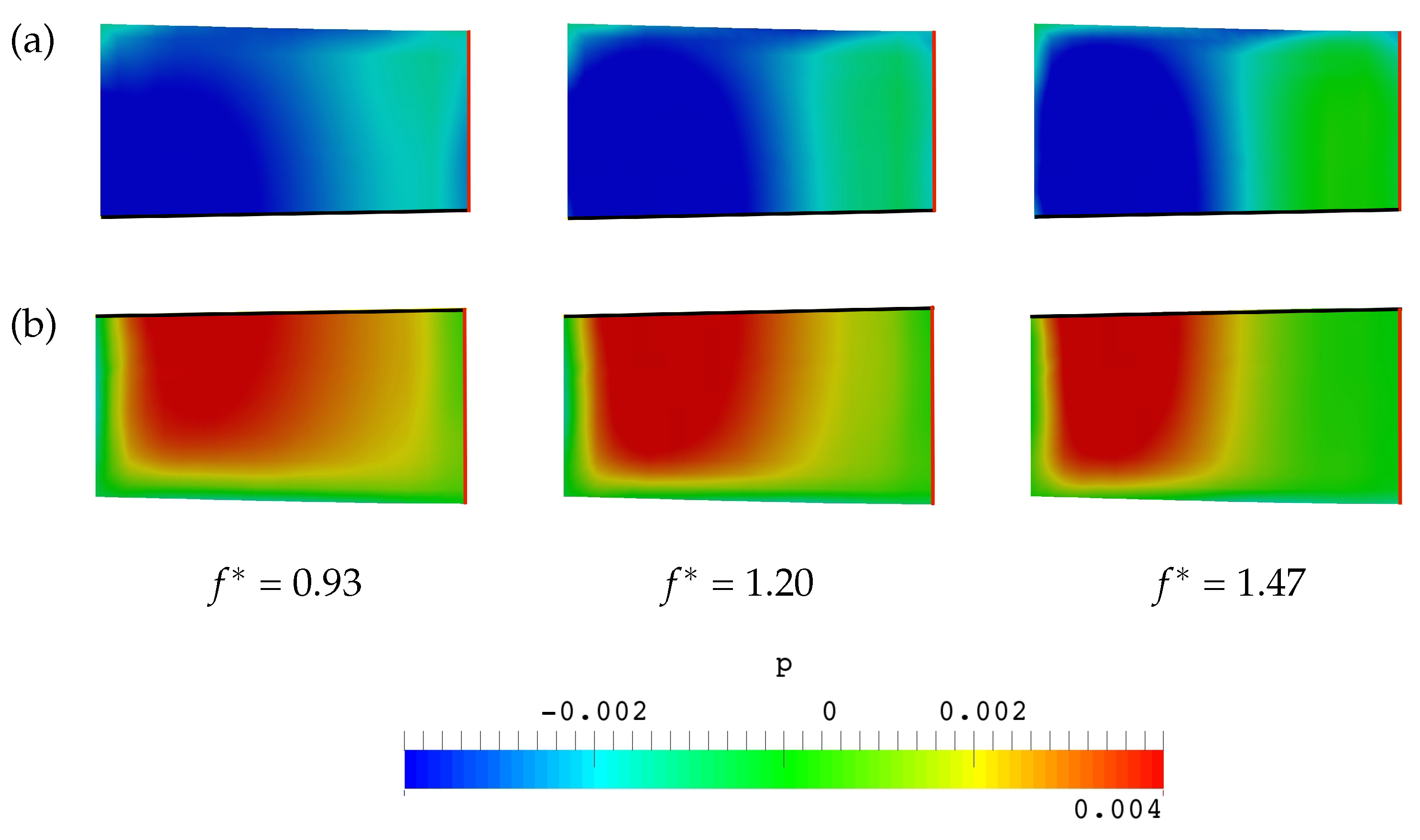
Figure 11a and Figure 12 show the comparison of pressure distribution on both sides of the plate surface for all cases at a phase instant when a peak value of positive thrust appears in all cases. The corresponding vortex structures around the plate are illustrated in Figure 11b. The phase instant at which a peak of positive thrust appears in each case can be seen in Figure 7, where points a, b and c are representative phase instants corresponding to $\varphi$ = 0.489, $\varphi$ = 0.561 and $\varphi$ = 0.611 for case 1, case 2 and case 3, respectively.

According to Figure 11a and Figure 12, the high pressure acting on the lower side of the plate in the case of an optimal frequency $f^{*}$ = 1.2 (case 2) is significantly larger than those in the other two cases. Consequently, case 2 exhibits the largest pressure difference among the three cases, which is consistent with the generation of the highest instantaneous positive thrust at the phase instant of $\varphi$ = 0.561 (point b in Figure 7) in case 2.

It is likely that the relative deformation of the trailing edge affects the distribution of pressure around the plate surface. When examining the pressure distribution on the plate surface of all cases, it is seen that the negative-pressure regions on the upper surface of the plate appear similar as seen in Figure 12a. It would seem that the positive-pressure region below the plate surface as seen in Figure 12b is creating the increase in thrust force.

In the case of $f^{*}$ = 0.93 (case 1), as shown in Figure 11a, the leading edge is at the phase instant of $\varphi$ = 0.489 and approaching the end of its acceleration phase with downward motion to its center. Meanwhile, the trailing edge is also on the way of a return stroke with downwards motion to its center in an acceleration phase. Since both the leading edge and trailing edge of the plate are in the accelerating phase with downward motion, the positive pressure is observed to be widely distributed along most of the lower surface of the plate.

From the first diagram of Figure 12b, it is seen that the positive-pressure region is enlarged from the leading edge to the trailing edge of the plate surface. Due to the relative velocity of the trailing edge and leading edge, asymmetric pressure is created on the lower surface of the plate. The positive-pressure field is more concentrated near the trailing edge region due to increasing displacement of the trailing edge. The pressure difference between the two surfaces is observed to be lowest among the three cases, which is consistent with the generation of smallest positive thrust in case 1. The lowest pressure difference in this case is attributed to the smallest relative displacement of trailing edge with that of leading edge as shown in Figure 6 (see point a).

In the cases of $f^{*}$ = 1.2 and $f^{*}$ = 1.47, the trailing edge exhibits out-of-phase motion and a shorter time of in-phase motion with the leading edge throughout most of a flapping stroke due to larger phase lag. As the $f^{*}$ increases, the high-pressure region on the lower surface of the plate shifts from the region near the leading edge to the region near the trailing edge and develops more around the trailing edge region as shown in Figure 11a.

As illustrated in Figure 11a, the leading edge of case 2 ($f^{*}$ = 1.2) is starting its second half-cycle with downward motion from its center position while the trailing edge is reversing its direction of motion to its center. Consequently, the leading edge is in a decelerating phase while the trailing edge is in an accelerating phase. Due to deceleration of the leading edge during its second half-cycle, it was observed that the positive pressure around half of the leading edge region dissipates while acceleration of the trailing edge leads to a notable development of positive pressure on most of the trailing edge region. The pressure difference between the two surfaces of the plate is observed to be the largest among the three cases, which is related to the generation of highest positive thrust at the phase instant of $\varphi$ = 0.561 (point b in Figure 7) in case 2. The reason for the largest pressure difference at this phase instant is consistent with the largest displacement of trailing edge relative to the leading edge as illustrated in Figure 6 (see point b).

As the $f^{*}$ increases, the out-of-phase motion of the trailing edge becomes more pronounced due to larger phase lag of the trailing edge. In Figure 11a, the leading edge of case 3 ($f^{*}$ = 1.47) is already on the way of its second half-cycle with downward motion from its center position while the trailing edge is at the beginning of its reverse motion to the center. Consequently, the leading edge is in a decelerating phase while the trailing edge is at the start of an accelerating phase. Deceleration of the leading edge causes most of its surrounding pressure to disappear. Meanwhile, the trailing edge is about to start its accelerating phase and delays to create a very large-pressure region along the lower surface of the plate. The positive pressure is observed to be mainly focused around the trailing edge region as shown in Figure 11a. When compared with case 2, this positive-pressure region in case 3 is observed to be smaller and hence the pressure difference in case 3 is also smaller. This seems to contribute to the lower value of maximum positive thrust in case 3 than in case 2. The above phenomenon is also reflected in the relative deformation of the trailing edge in comparison of case 2 with case 3 (see points b and c in Figure 6).

The difference in phase lag, which causes the difference in relative deformation of the trailing edge with respect to the leading edge, is found to be a key factor in estimating the flow field and associated thrust production. The optimal phase lag for maximum thrust production may be associated with the maximum relative deformation. Thrust force was shown to enhance when the motion of trailing edge is out of phase with that of leading edge.

Figure 13 shows a comparison of the pressure distribution on both sides of the plate surface for all cases at a phase instant when a peak value of negative thrust appears in each case. The phase instant at which a peak of negative thrust appears in each case is presented in Figure 7, where points d, e, and f are representative phase instants corresponding to $\varphi$ = 0.244, $\varphi$ = 0.318 and $\varphi$ = 0.358 for case 1, case 2 and case 3, respectively. The generation of negative thrust in each case is also reflected in the relative deformation of the trailing edge as shown in Figure 6, where the phase instant of the minimum thrust force in each case is marked with black squares.

At these phase instants, it is observed that the plate holds the circular low-pressure region closer to its trailing edge, which results in a significant decrease in thrust force. However, these low-pressure regions seem quite similar in all cases, especially in cases 2 and 3. This similarities can be confirmed by the TEV structure as shown in the front and top views of Figure 14a,b. It would seem that an extra increase in negative thrust arises from the pressure difference created near the leading edge region. Due to the pressure difference created near the leading edge region, the plate cannot push the water sufficiently backward to produce forward motion, which seems to cause an extra increase in negative value of thrust in cases 2 and 3 at these phase instants.

For the case of $f^{*}$ = 0.93 (case 1), the leading edge is approaching the end of its decelerating phase with upward motion from the center position and its velocity is approaching zero. This results in the decaying of the positive and negative pressure around the leading edge and a slight difference in pressure distribution is observed around the leading edge as shown in Figure 13a.

For the cases of $f^{*}$ = 1.2 and $f^{*}$ = 1.47 (case 2 and 3), the leading edge is in an accelerating phase with downward motion to its center position and its velocity is increasing to maximum. In these two cases, the generation of positive and negative pressure can be observed clearly around the leading edge as shown in Figure 13b,c. Among the three cases, the pressure difference, which is mainly developed near the leading edge, is observed to be largest in case 3. This largest pressure difference acts to push the plate backward, which is consistent with a massive increase in negative value of thrust at this phase instant of case 3. The largest value of negative thrust in case 3 is observed to be associated with the largest negative value of relative deformation as shown in Figure 6 (see point f).

4. Conclusions

The flow field of a basic caudal-fin model, a square flexible flapping plate, was simulated numerically. The leading edge of the plate was set to oscillate vertically in a stationary tank. The plate’s motion was simulated in three dimensions using open-source CFD software. The numerical analysis was performed over a range of flapping frequencies that exist near resonance. Good quantitative agreement was found between the calculated and experimental results for the trailing edge amplitude of the plate and phase lag of the trailing edge relative to the leading edge. This study provides an explanation regarding how the flexible plate obtains forward thrust in sinusoidal flapping motion.

By analyzing the pressure distribution and deformation of the plate, the generation of thrust in a sinusoidal flapping motion was clarified in detail. It was found that the formation of the pressure difference between the upper and lower surfaces of the plate is related to the generation of both positive- and negative-thrust forces during the flapping period of the plate motion. The phase difference, the difference in relative displacement between the trailing and leading edges, changes the instantaneous pressure distribution on the plate surface during the flapping period and strongly affects the generation of both positive- and negative-thrust forces. It was observed that the optimal phase difference for maximum thrust was associated with the maximum relative displacement of the trailing edge to the leading edge. Within the range of non-dimensional flapping frequencies 0.93 $<f^{*}<$ 1.47, the combination of phase difference information and relative deformation of the trailing edge may improve the thrust of a flapping plate. The results of the current simulations may provide new guidelines for improving the design of robotic underwater vehicles.

References

1. Lauder, G.V.; Anderson, E.J.; Tangorra, J.; Madden, P.G. Fish biorobotics: Kinematics and hydrodynamics of self-propulsion. J. Exp. Biol. 2007, 210, 2767–2780. [Google Scholar] [CrossRef] [PubMed] [Green Version]
2. Xin, Z.; Wu, C. Shape optimization of the caudal fin of the three-dimensional self-propelled swimming fish. Sci. China Phys. Mech. Astron. 2013, 56, 328–339. [Google Scholar] [CrossRef]
3. Ren, Z.; Hu, K.; Wang, T.; Wen, L. Investigation of fish caudal fin locomotion using a bio-inspired robotic model. Int. J. Adv. Robot. Syst. 2016, 13, 87. [Google Scholar] [CrossRef] [Green Version]
4. Li, N.; Su, Y. Fluid dynamics of biomimetic pectoral fin propulsion using immersed boundary method. Appl. Bionics Biomech. 2016, 2016, 2721968. [Google Scholar] [CrossRef] [PubMed] [Green Version]
5. Luo, Y.; Xiao, Q.; Shi, G.; Pan, G.; Chen, D. The effect of variable stiffness of tuna-like fish body and fin on swimming performance. Bioinspir. Biomim. 2020, 16, 016003. [Google Scholar] [CrossRef]
6. Arora, N.; Gupta, A.; Sanghi, S.; Aono, H.; Shyy, W. Flow patterns and efficiency-power characteristics of a self-propelled, heaving rigid flat plate. J. Fluids Struct. 2016, 66, 517–542. [Google Scholar] [CrossRef]
7. Li, R.; Xiao, Q.; Liu, Y.; Li, L.; Liu, H. Computational investigation on a self-propelled pufferfish driven by multiple fins. Ocean. Eng. 2020, 197, 106908. [Google Scholar] [CrossRef]
8. Wan, H.; Dong, H.; Gai, K. Computational investigation of cicada aerodynamics in forward flight. J. R. Soc. Interface 2015, 12, 20141116. [Google Scholar] [CrossRef] [Green Version]
9. Fei, Y.-H.J.; Yang, J.-T. Enhanced thrust and speed revealed in the forward flight of a butterfly with transient body translation. Phys. Rev. E 2015, 92, 033004. [Google Scholar] [CrossRef]
10. Paraz, F.; Schouveiler, L.; Eloy, C. Thrust generation by a heaving flexible foil: Resonance, nonlinearities, and optimality. Phys. Fluids 2016, 28, 011903. [Google Scholar] [CrossRef]
11. Kato, K. PIV Measurements in Complex Flows Bounded by Deforming Surface. Master’s Thesis, Keio University, Yokohama, Japan, 2010. [Google Scholar]
12. Quinn, D.B.; Lauder, G.V.; Smits, A.J. Scaling the propulsive performance of heaving flexible panels. J. Fluid Mech. 2014, 738, 250–267. [Google Scholar] [CrossRef] [Green Version]
13. Leftwich, M.C.; Tytell, E.D.; Cohen, A.H.; Smits, A.J. Wake structures behind a swimming robotic lamprey with a passively flexible tail. J. Exp. Biol. 2012, 215, 416–425. [Google Scholar] [CrossRef] [Green Version]
14. Spagnolie, S.E.; Moret, L.; Shelley, M.J.; Zhang, J. Surprising behaviors in flapping locomotion with passive pitching. Phys. Fluids 2010, 22, 041903. [Google Scholar] [CrossRef] [Green Version]
15. Hoover, A.P.; Cortez, R.; Tytell, E.D.; Fauci, L.J. Swimming performance, resonance and shape evolution in heaving flexible panels. J. Fluid Mech. 2018, 847, 386–416. [Google Scholar] [CrossRef] [Green Version]
16. Michelin, S.; Llewellyn Smith, S.G. Resonance and propulsion performance of a heaving flexible wing. Phys. Fluids 2009, 21, 071902. [Google Scholar] [CrossRef] [Green Version]
17. Fernandez-Feria, R.; Alaminos-Quesada, J. Analytical results for the propulsion performance of a flexible foil with prescribed pitching and heaving motions and passive small deflection. J. Fluid Mech. 2021, 910. [Google Scholar] [CrossRef]
18. Floryan, D.; Rowley, C.W. Clarifying the relationship between efficiency and resonance for flexible inertial swimmers. J. Fluid Mech. 2018, 853, 271–300. [Google Scholar] [CrossRef] [Green Version]
19. Ramananarivo, S.; Godoy-Diana, R.; Thiria, B. Rather than resonance, flapping wing flyers may play on aerodynamics to improve performance. Proc. Natl. Acad. Sci. USA 2011, 108, 5964–5969. [Google Scholar] [CrossRef] [PubMed] [Green Version]
20. Thiria, B.; Godoy-Diana, R. How wing compliance drives the efficiency of self-propelled flapping flyers. Phys. Rev. E 2010, 82, 015303. [Google Scholar] [CrossRef] [PubMed] [Green Version]
21. Zhu, X.; He, G.; Zhang, X. Numerical study on hydrodynamic effect of flexibility in a self-propelled plunging foil. Comput. Fluids 2014, 97, 1–20. [Google Scholar] [CrossRef]
22. Masoud, H.; Alexeev, A. Resonance of flexible flapping wings at low Reynolds number. Phys. Rev. E 2010, 81, 056304. [Google Scholar] [CrossRef] [Green Version]
23. Dewey, P.A.; Boschitsch, B.M.; Moored, K.W.; Stone, H.A.; Smits, A.J. Scaling laws for the thrust production of flexible pitching panels. J. Fluid Mech. 2013, 732, 29–46. [Google Scholar] [CrossRef]
24. Gibouin, F.; Raufaste, C.; Bouret, Y.; Argentina, M. Study of the thrust–drag balance with a swimming robotic fish. Phys. Fluids 2018, 30, 091901. [Google Scholar] [CrossRef] [Green Version]
25. Baba, N.; Obi, S. Experimental study on modeled caudal fins propelling by elastic deformation. In Proceedings of the ASME 2018 5th Joint US-European Fluids Engineering Summer Conference, Montreal, QC, Canada, 15–20 July 2018; Volume 51555, p. V001T02A007. [Google Scholar]
26. Karimnejad, S.; Delouei, A.A.; Basagaoglu, H.; Nazari, M.; Shahmardan, M.; Falcucci, G.; Lauricella, M.; Succi, M. A Review on contact and collision methods for multi-body hydrodynamic problems in complex flows. Commun. Comput. Phys. 2022, 32, 899–950. [Google Scholar] [CrossRef]
27. Afra, B.; Delouei, A.A.; Mostafavi, M.; Tarokh, A. Fluid–structure interaction for the flexible filament’s propulsion hanging in the free stream. J. Mol. Liq. 2021, 323, 114941. [Google Scholar] [CrossRef]
28. Tukovic, Ž.; Karač, A.; Cardiff, P.; Jasak, H.; Ivankovic, A. OpenFOAM finite volume solver for fluid-solid interaction. Trans. FAMENA 2018, 42, 1–31. [Google Scholar] [CrossRef]
29. Khin, M.H.W.; Kato, K.; Sung, H.J.; Obi, S. Fluid flow induced by an elastic plate in heaving motion. ASEAN Eng. J. 2022, 12, 1–9. [Google Scholar] [CrossRef]
Figure 1. Schematic view of a square flexible plate. The leading edge is indicated by the red line and the trailing edge is indicated by the blue line.
Applsci 12 12693 g001
Figure 2. (a) Schematic view of a computational domain. (b) Grid generation. The leading edge and symmetry plane of the plate are indicated by red and yellow lines, respectively. The origin of coordinate is at the center of the leading edge of the plate.
Applsci 12 12693 g002
Figure 3. Comparison between the simulation and experiment for different: (a) Trailing edge amplitude A t . (b) Phase lag of the plate ϕ l a g .
Applsci 12 12693 g003
Figure 4. Comparison on the displacement of trailing edge with three different mesh resolutions.
Applsci 12 12693 g004
Figure 5. (a) Mean thrust. (b) The maximum relative deformation of trailing edge δ m a x for different non-dimensional frequencies f * .
Applsci 12 12693 g005
Figure 6. Displacement of the trailing edge relative to the leading edge, z t z r , for different f * in a flapping cycle.
Applsci 12 12693 g006
Figure 7. Instantaneous thrust variation with different f * in a flapping cycle.
Applsci 12 12693 g007
Figure 8. Variation of mean thrust coefficient with different f * .
Applsci 12 12693 g008
Figure 9. Pressure distributions on the spanwise symmetry plane of the plate during a half-flapping cycle for the case of f * = 0.93 (case 1).
Applsci 12 12693 g009
Figure 10. Three-dimensional vortex structures around the plate during a half-flapping cycle for the case of f * = 0.93 (case 1).
Applsci 12 12693 g010
Figure 11. (a) Pressure distributions on the spanwise symmetry plane of the plate and (b) three-dimensional vortex structures at the phase instant when a peak value of thrust appears in each case.
Applsci 12 12693 g011
Figure 12. Pressure distributions on the; (a) top and (b) bottom surfaces of the plate at a phase instant when a peak value of positive thrust appears in each case (The symmetry plane and leading edge are represented by a black line and red line, respectively).
Applsci 12 12693 g012
Figure 13. Pressure distributions on the spanwise symmetry plane of the plate at a phase instant when a peak value of negative thrust appears for the case of: (a) f * = 0.93. (b) f * = 1.2. (c) f * = 1.47.
Applsci 12 12693 g013
Figure 14. (a) Front view and (b) bottom view of three-dimensional vortex structures at the phase instant when a peak value of thrust appears for the cases of; f * = 0.93, f * = 1.20 and f * = 1.47.
Applsci 12 12693 g014