Off-Axis Holographic Interferometer with Ensemble Deep Learning for Biological Tissues Identification

Abstract

This paper proposes a method with an off-axis interferometer and an ensemble deep learning (I-EDL) hologram-classifier to interpret noisy digital holograms captured from the tissues of flawed biological specimens. The holograms are captured by an interferometer, which serves as a digital holographic scanner to scan the tissue with 3D information. The method achieves a high success rate of 99.60% in identifying the specimens through the tissue holograms. It is found that the ensemble deep learning hologram-classifier can effectively adapt to optical aberration coming from dust on mirrors and optical lens aberrations such as the Airy-plaque-like rings out-turn from the lenses in the interferometer. The deep learning network effectively adapts to these irregularities during the training stage and performs well in the later recognition stage without prior optical background compensations. The method does not require an intact sample with a full outline shape of the specimens or the organs to understand the objects’ identities. It demonstrates a new paradigm in object identification by ensemble deep learning through a direct wavefront recognition technique.

1. Introduction

The advancements in optics and computing technologies have enabled digital holograms of physical three-dimensional (3D) objects to be captured and analyzed at high speed and achieve close to real-time response performance. Holograms can be displayed with a spatial light modulator to reconstruct a visible image and is an ideal solution for recording, storing, and displaying 3D objects in the digital world. However, a hologram comprises high-frequency fringe patterns and is almost impossible to recognize with traditional computer vision methods. Furthermore, in many practical situations, intact extraction of a biological specimen or organ is not feasible, and therefore the object’s identity cannot be inferred directly from its outline shape. However, a digital holographic interferometer is an effective hologram-capturing device to examine the microstructure inside a specimen. Furthermore, the off-axis configuration simplifies the difficulties of separating a hologram’s zero-order image from the two conjugate virtual and real images in Fourier space.

During the early stage of optical hologram classification methods, almost all methods were based on correlation, where a targeted hologram is matched against a library of reference hologram templates. The matching is generally realized with optical correlation and only results in a high matching score if a pair of objects have similar poses and depth. Most of these approaches are sensitive to positional shifts and deformations. The methods and the problems are described in detail by VanderLugt works in [1] and the articles in [2,3,4,5]. The hologram classifier employed in this paper is EDL-IOHC [6], in which a modern deep learning approach is employed. The feature extraction process of the deep learning approach is fully automated. The method solves most of the shift-invariant problems within a single framework with the capability to handle occlusion problems effectively.

Nowadays, some researchers are using the common term Hologram interchangeably with the terms ‘Raw Hologram’ and ‘Digital Hologram’. In order to avoid potential confusion, the following definitions explicitly state the difference in their meanings. ‘Raw Hologram’ is the intensity map recorded on a camera or a film, and usually, this intensity map will be used for the object wavefront reconstruction, as Dennis Gabor showed in his works in 1948 [7]. ‘Digital Hologram’ is a representation of the complex optical wavefront diffracted from an object. The complex wavefront is either generated directly by a computer or reconstructed digitally from a ‘Raw Hologram’. A computer-generated hologram is often referred to as wavefront-based CGH [8], Computer Generated Hologram, starting from the works by J.W. Goodman and R.W. Lawrence [9] during the period of the mid-1960s.

A basic tool in two-dimensional digital signal processing used in digital holography is DFT (discrete Fourier transform) and the corresponding IDFT (inverse discrete Fourier transform), making fast computation possible. For raw holograms captured by a modern digital camera, their corresponding frequency spectrums are also discrete. The DFT transforms the raw hologram from the spatial domain to the frequency domain in a discrete manner. The raw hologram spectrum and the corresponding object wavefront extraction methods have been reported in detail in numerous works in the literature, such as [10,11,12,13]. In the frequency domain of a raw hologram, the spectrums of the zero-order image, virtual image, and real image are shifted and separated by the off-axis configuration. As a result, the object wavefront (digital hologram) can be extracted relatively easily.

In this paper, we have proposed a novel technique for identifying biological samples based on their tissues’ digital holograms. The paper is organized as follows. In Section 2, a detailed optical setup of a single-shot off-axis digital holographic interferometer, an outline of the digital hologram-classifier EDL-IOHC in [14], and the workflow of converting a raw hologram to a digital hologram are described. Experimental results are presented in Section 3. A conclusion summarizing the essential findings is given in Section 4.

2. Method

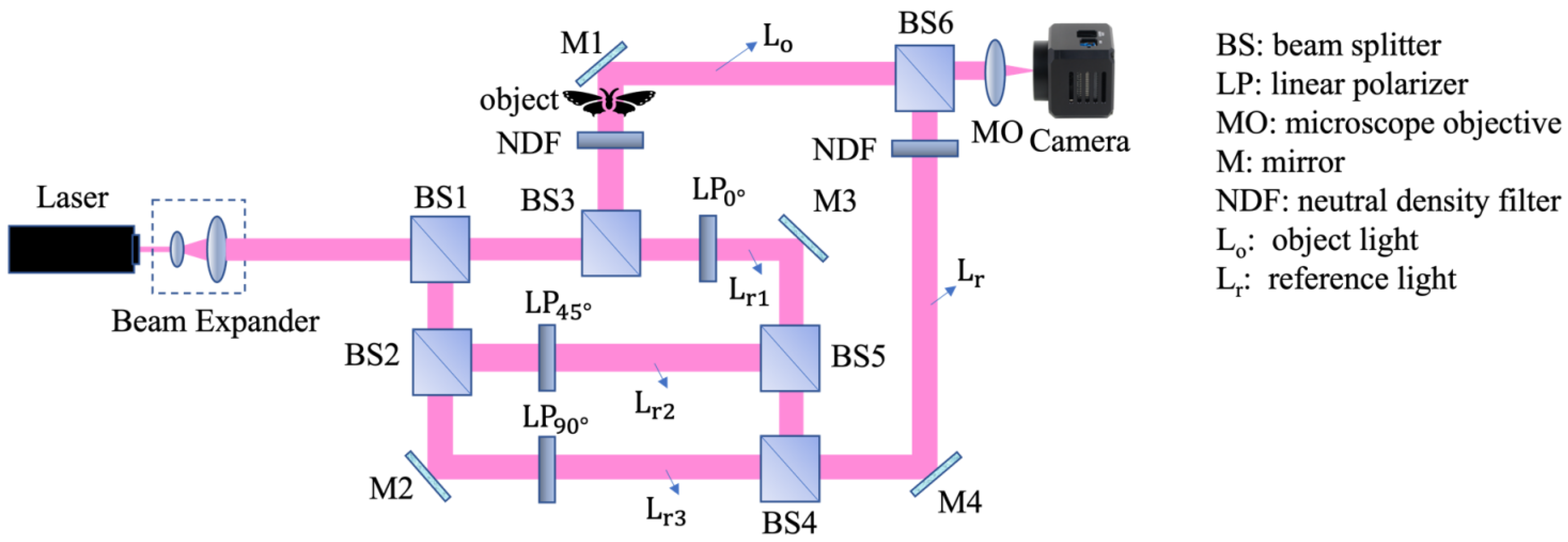
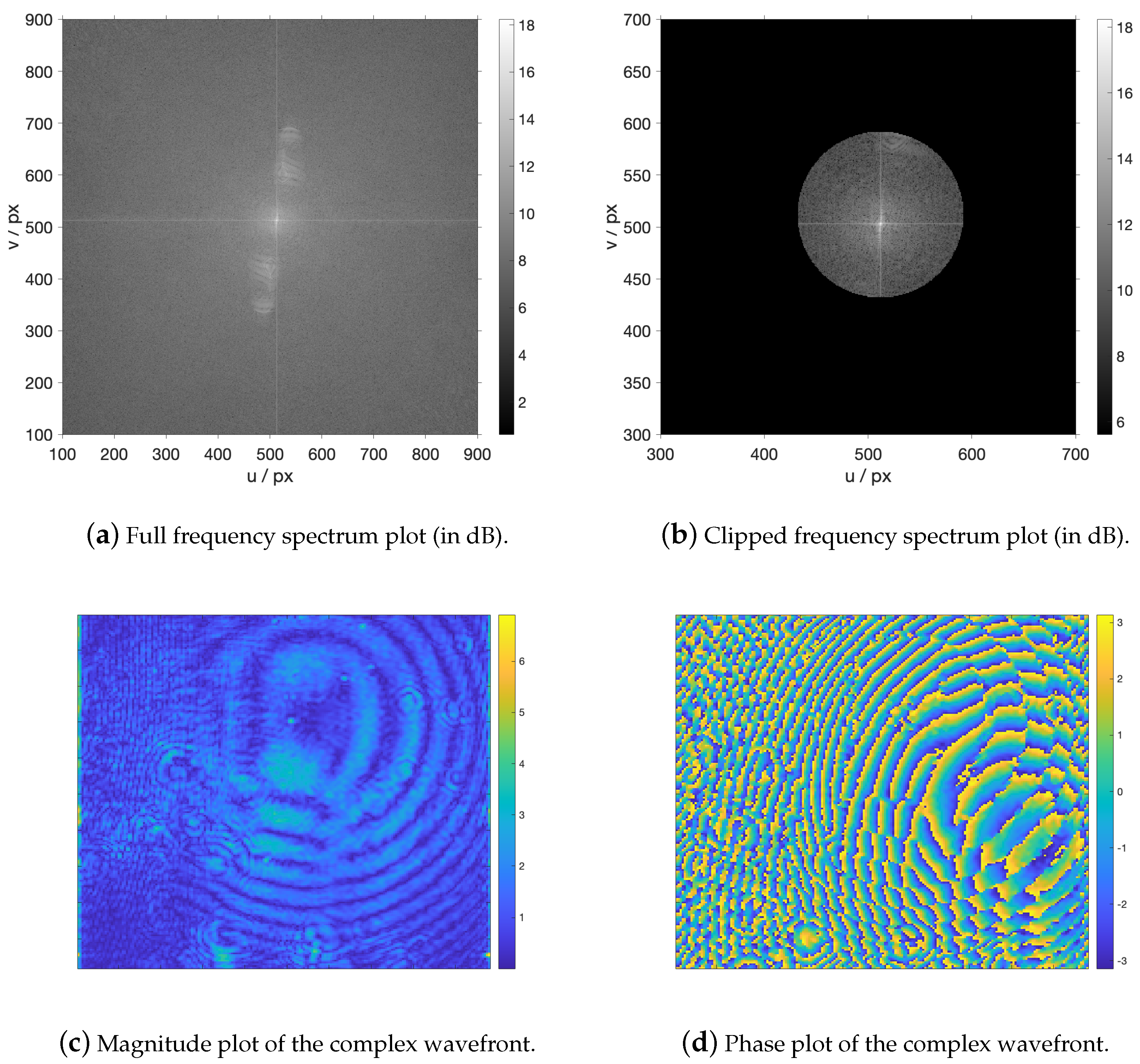
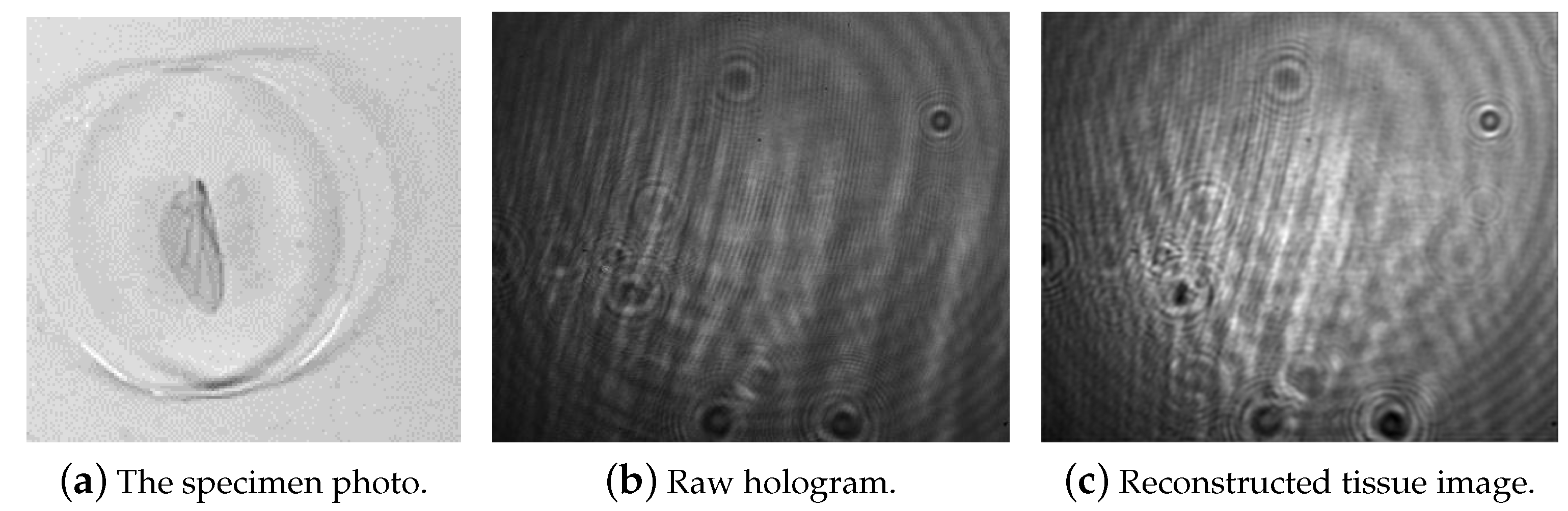
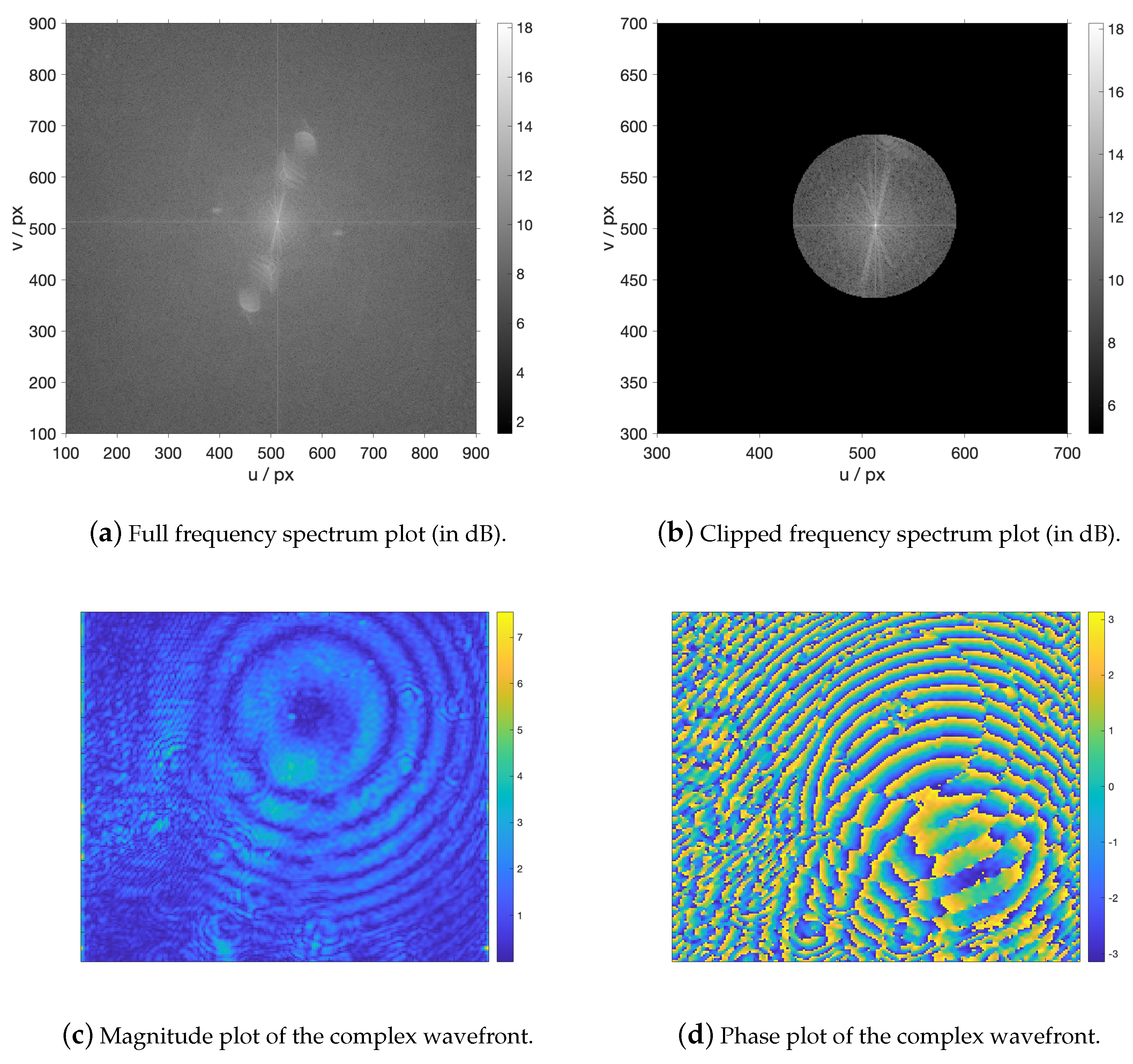
2.1. Single-Shot Off-Axis Digital Holographic Interferometer

Our proposed interferometer and ensemble deep learning (I-EDL) method consisted of a single-shot off-axis digital holographic interferometer and an ensemble deep learning system for raw hologram capturing and complex object wavefront recognition. The interferometer provides off-axis holograms with a shifted spectrum of the object’s real image that can be easily extracted and processed by the fast Fourier transform method, which is explained in detail by [10,11]. The optical setup is based on the principle of spatial coherence and is installed on a curtain-enclosed optical table [15]. The coherent light source is a red He-Ne laser with a wavelength of $632.8$ nm [14], and the laser beam is approximately 2 mm in diameter. The object light formed by a laser beam passes through the tissue specimen and records the object information related to it. Change the specimen positions in x-y directions and record hundreds of experimental data images. The holograms are captured by a CMOS camera equipped with a Nikon Plan microscope objective [16]. The following Figure 1 shows a schematic diagram of the optical setup in detail, where MO is a microscopic objective, and NDF is a neutral density filter. The reference light is separated by several beam splitters (BS2, BS3) into three light beams and polarized by three linear polarizers (LP$0^{\circ }$, LP${45}^{\circ }$, and LP${90}^{\circ }$) under 0${}^{\circ }$, 45${}^{\circ }$, and 90${}^{\circ }$, respectively. Then, they are combined by BS4 and BS5 and interfere with the object light to form the fringe image. The system employs two neutral density filters in the object light beam (Lo) and references light beam (Lr) to adjust the light intensity from overexposure. The raw hologram of the object is recorded by the camera. Compared with a standard off-axis system, the setup can get raw holograms with different polarization states in a single shot, reduces image degradation due to light scatterings, and has higher imaging efficiency. The extra polarization information is capable of image denoising and more details can be found in [17].

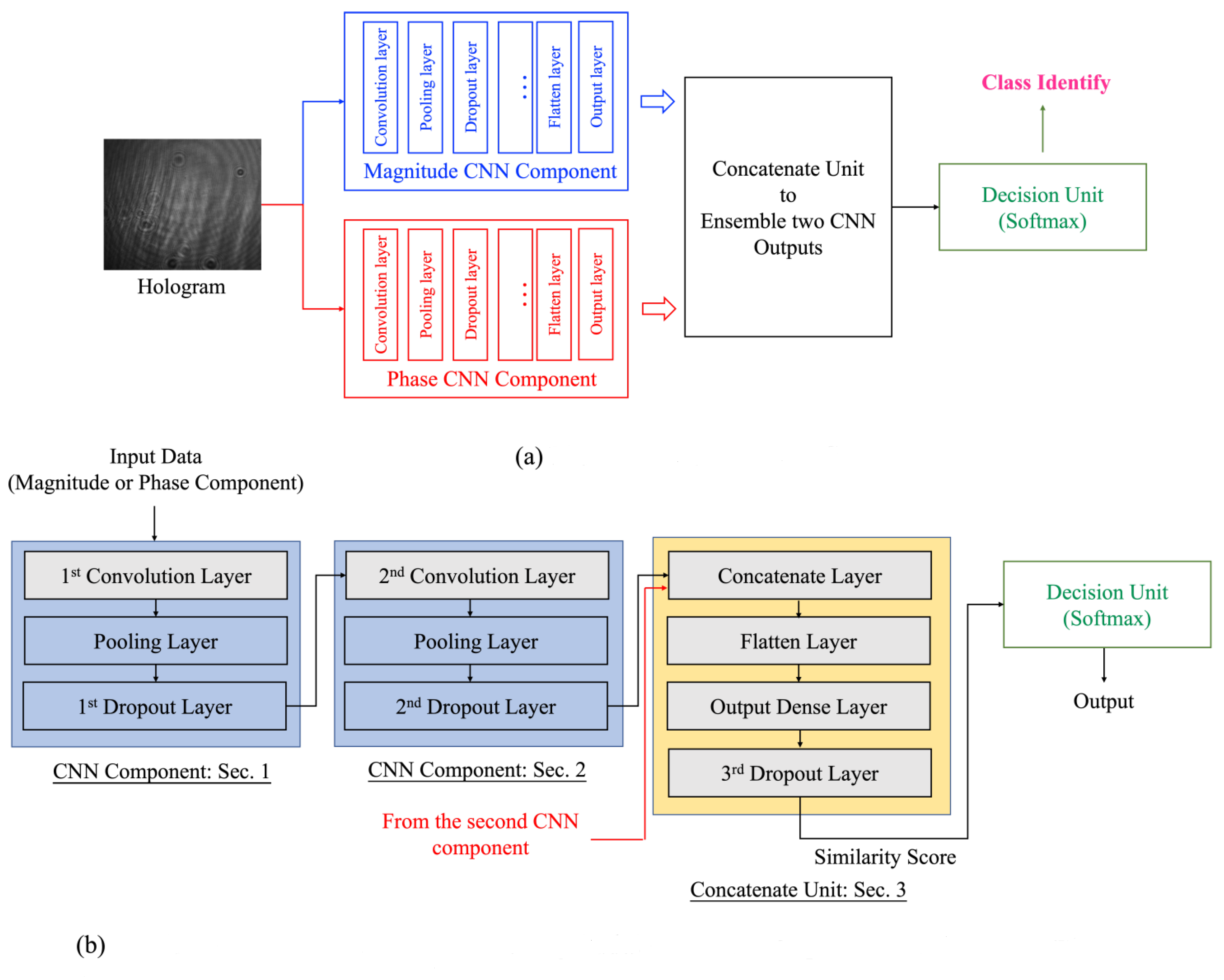
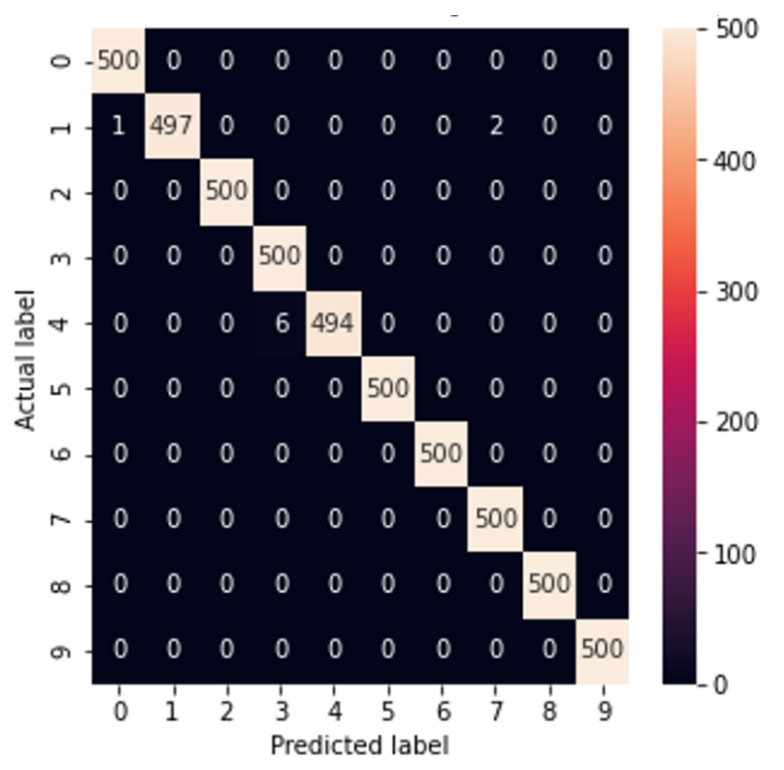
2.2. Ensemble Deep-Learning Network

The hologram-classifier employed in this paper is EDL-IOHC. The approach in the articles [18,19] opens a new paradigm for digital hologram recognition directly by wavefront analysis. The choice of EDL-IOHC is due to its robustness and high accuracy under noisy conditions with occlusion compared to its predecessors in [18,19]. For clarity of explanation, the hologram-classifier EDL-IOHC, a complex wavefront recognition system, is outlined below.

In reference to Figure 2a, which shows the structure of EDL-IOHC in [6] for recognizing digital holograms with the powerful capability to handle occluded objects contaminated with speckle noise. The input of the network is the reconstructed hologram with both magnitude and phase information, as shown in Figure 2a. The first and second CNN, known as the Magnitude CNN and the Phase CNN, accept the magnitude and phase components of the digital hologram, which is structurally the same but trained with different components’ information. The architecture of both CNNs, as shown in Figure 2b, can be divided into three sections. Section 1 and Section 2 have identical structures but different hyper-parameters, containing a convolution layer for local feature extraction, max-pooling, and dropout layers. Section 3 is a shared section for both the CNNs, and it is a “Concatenate Unit” to ensemble output information from the two CNNs. The concatenate unit ensembles all the extracted phase features and magnitude features into a combined flatten features vector before fitting into the “Output Dense Layer” for the decision unit to output the identity of the input digital hologram.

This study employs the hologram-classifier EDL-IHC to identify the tissue object wavefronts (digital holograms) reconstructed from the raw intensity fringe patterns.

Fringe pattern intensity is referred to as a raw hologram; $\Gamma$ is a real number quantity and can be obtained as the result of measuring the intensity that results from the linear superposition of a diffracted object wavefront ‘O’ and a reference wavefront ‘R’. Mathematically, the recorded intensity image can be expressed as follows:

$$\Gamma (m,n)={∥R(m,n)+O(m,n)∥}^2$$

(1)

where $\Gamma (m,n)$ is the intensity of the captured hologram with a size of M columns × N rows. $R(m,n)$ is the reference wavefront, and $O(m,n)$ is the object wavefront.

Expanding Equation (1) is as follows:

$$\begin{array}{cc}\hfill \Gamma (m,n)=& {∥R(m,n)∥}^2+{∥O(m,n)∥}^2\hfill \\ & +O(m,n)R^{*}(m,n)+O^{*}(m,n)R(m,n)\hfill \end{array}$$

(2)

where * is the complex conjugate operation for complex numbers, ${∥R(m,n)∥}^2$ is the square magnitude of the reference wavefront, and ${∥O(m,n)∥}^2$ is the square magnitude of the object wavefront. $\Gamma$ is a set of dark and bright fringes that embeds the amplitude and the phase information of the corresponding complex object wavefront.

Discrete Fourier Transform (DFT) is performed on the off-axis raw hologram and generates the four terms in the frequency domain. The DFT transforms the raw hologram from the spatial domain to the frequency domain in a discrete manner. After performing DFT on Equation (2) and getting Equation (3), as below.

$$\begin{array}{cc}\hfill H(u,v)=& A^{2}MN\delta (u,v)+DFT\left\{{∥O(m,n)∥}^2\right\}\hfill \\ & +DFT\left\{O\left(m,n\right)R^{*}(m,n)+O^{*}\left(m,n\right)R(m,n)\right\}\hfill \end{array}$$

(3)

where $u,v$ are the frequency axis, $\delta (*)$ is the delta function, and A is the reference wave’s amplitude.

In the frequency domain, the spectral locations of the frequency components separated by the recorded off-axis hologram provide easy means to separate specific wavefront information in the Fourier space. The spectrum in the third term is extracted by a masking method, and the zero-order low-frequency spectrum and the twin image spectrum are removed. The third term extracted spectrum $DFT\left\{O\left(m,n\right)R^{*}(m,n)\right\}$, as shown in Equation (3), is centered (the masking method and centering algorithm is introduced in [10] with great detail), and then inverse Fourier transform is performed and get the scaled complex object wavefront $AO(m,n)$, which is the object wavefront multiplied by the reference wave with amplitude A. Then, a ‘min-max’ normalization algorithm [20] is applied to A. This method of normalization algorithm used in the machine learning community scales the values in a data array from [minimum value, maximum value] to [$-1$, 1] through a linear mapping. It normalizes the effect of the scalar multiplication by the reference wave for recognition. The normalization provides a robust pre-processing method for recognition purposes. In the following Figure 3 illustrates the procedures to get the object wavefront (the digital hologram) for training the EDL-IOHC deep learning network.

Raw holograms of the tissue are captured from the biological samples. Fast DFT transforms the raw holograms from the spatial domain to the frequency domain. The spectrums of the object wavefronts are extracted, and fast IDFT restores the spectrums into the object wavefronts. The object wavefront extraction methods from raw holograms have been reported in [10,11,12,13] with details. The object wavefront extracted from the above process is a complex quantity that contains both the magnitude and phase components of the object wave $O(m,n)$, a digital hologram. The full dataset is split into an in-training train set and an out-training test set. The EDL-IOHC is trained with the train set and tested by the test set. It is found that aberrations have come from dust on optical lenses and mirrors, Airy-plaque-like rings [21] out-turn from the system’s lenses. However, the deep learning network can adapt to these background irregularities during the first training stage and continue to perform well in the later recognition stage without any necessary background compensation.

Ten different types of tissues are captured from ten different types of flawed biological specimens, which are Cucurbita Stem, Pine Stem, Corn (Zea Mays) Seed, House Fly Wing, Honeybee Wing, Bird Feather, Corpus Ventriculi, Liver Section, Lymph Node and Human Chromosome with their class labels shown in

Table 1. The class labels for different specimens.

Specimen Class	Class Label
Cucurbita Stem	0
Pine Stem	1
Corn (Zea mays) Seed	2
House Fly Wing	3
Honeybee Wing	4
Bird Feather	5
Corpus Ventriculi	6
Liver Section	7
Lymph Node	8
Human Chromosome	9

.

Five hundred raw holograms are captured from tissues of each class of the ten biological specimens and result in a total dataset size of 5000 digital holograms (object wavefront). They are used to train the hologram-classifier EDL-IOHC. Then, the trained hologram-classifier is used to identify the type of biological specimens by recognizing the tissues’ digital holograms.

3. Experiments

The system consisted of a computer equipped with an i-7 Intel processor, Nvidia RTX 2080 Super GPU with 384 Tensor cores, the interferometer, a microscope objective, and a CMOS camera. The hologram-classifier uses the same set of hyperparameters of the EDL-IOHC reported in [6]. The new optical parameters for the digital holographic interferometric system are shown in

Table 2. Optical parameters of the digital holographic interferometer system.

Optical Parameters	Values
Wavelength of light	$632.8$ nm
Pixel size	3.45 $\mathsf{\mu }$m
Size of hologram	2056 rows × 2546 columns
Off-axis angle	1.5 degrees

.

As illustrations, Figure 4, Figure 5, Figure 6, Figure 7 and Figure 8 show examples from the human chromosome and the house fly wing datasets. Figure 4 and Figure 6 are the corresponding images. Figure 5 and Figure 7 are 3D plots of the spectrums and complex wavefront as a better means of visualization as they are not typical interpretable visual images but are a 2D array of complex phasors. The chromosome is close to transparent, and it is one of the most challenging samples to be separated if not using a hologram-classifier. The house fly wing is semitransparent, and the phase information can complement the magnitude information to build better decision boundaries for the deep learning network.

From the full dataset of size 5000 capture raw holograms, 5000 digital holograms (complex object wavefront) are extracted. Then 4000 out of the 5000 are taken as the in-training dataset, while the remaining out-training dataset is used as a test set. The ensemble CNN is trained with 3200 in-training set data, and the remaining 800 are used as a validation set to stop the training process by an early stopping mechanism. Finally, both the in-training dataset and the out-training dataset are used to evaluate the hologram-classifier. Training is stopped by the validation set when the change of the validating accuracy is less than 0.01%.

The ensemble CNN is trained by the dataset with cosine smoothing on the phase components, the validating set stops the training epoch, and the actual epoch run is 16. In each epoch, the holograms in the in-training set of the dataset are used to train the deep learning structure. The trained structure is then applied to classify the datasets. The following confusion matrix in Figure 8 shows that eight out of the ten classes are correct with very high overall classification accuracy, as shown in

Table 3. Success rates for classifying the out-training test set and the complete dataset by the EDL-IOHC hologram-classifier.

Dataset	Success Rate
Test set	99.60%
Complete set (both out- and in-training sets)	99.82%

.

The results in Table 3 reflect that in classifying the object, EDL-IOHC can maintain a high success rate of 99.60% for the out-training test set and 99.82% for the entire dataset. The performance is better than the benchmarking experiment conducted in [6] on partially occluded digit objects with speckle noise contamination.

4. Conclusions

This paper proposes a hologram-classifier on the digital hologram obtained by an off-axis interferometer from biological specimen tissues. The method does not require an intact sample with a complete outline shape of the specimens or the organs to understand the objects’ identities and achieves a high success rate of 99.60% on the out-training test set, and is able to adapt for optical aberrations from lenses and mirrors without prior background compensations. The result demonstrates that the hologram-classifier EDL-IOHC is robust under noisy and imperfect holography optical processes, and the off-axis interferometer is effective for scanning the microstructure of the tissues from the specimens. The simplicity of direct application in recognition of biological specimen tissue by EDL-IOHC, without any changes in architectural or hyperparameters, verified the generality of EDL-IOHC. In passing, more potential applications such as pollutant plastics, defective glasses, or identification of infected red blood cells from normal cells will be feasible by using EDL-IHC with a similar interferometer. Intuitively the biological specimen tissue hologram looks noisy and challenging. However, it is numerically not more challenging than the occluded simple digit patterns with speckle noise tested in the EDL-IOHC. Furthermore, for potential applications that require more compact size and lower cost but could accept lower performance, a smaller on-axis inline interferometer could also be considered. The method demonstrates a new paradigm in object identification by ensemble deep learning through the EDL-IOHC wavefront recognition technique.

References

1. Lugt, A.V. Signal detection by complex spatial filtering. IEEE Trans. Inf. Theory 1964, 10, 139–145. [Google Scholar] [CrossRef]
2. Poon, T.C.; Kim, T. Optical image recognition of three-dimensional objects. Appl. Opt. 1999, 38, 370–381. [Google Scholar] [CrossRef] [PubMed] [Green Version]
3. Kim, T.; Poon, T.C. Extraction of 3-D location of matched 3-D object using power fringe-adjusted filtering and Wigner analysis. Opt. Eng. 1999, 38, 2176–2183. [Google Scholar] [CrossRef]
4. Kim, T.; Poon, T.C. Three-dimensional matching by use of phase-only holographic information and the Wigner distribution. JOSA A 2000, 17, 2520–2528. [Google Scholar] [CrossRef] [PubMed]
5. Park, S.C.; Lee, K.J.; Lee, S.H.; Kim, S.C.; Kim, E.S. Robust recognition of partially occluded 3-D objects from computationally reconstructed hologram by using a spatial filtering scheme. In Proceedings of the Practical Holography XXIII: Materials and Applications; SPIE: Bellingham, WA, USA, 2009; Volume 7233, pp. 254–262. [Google Scholar]
6. Lam, H.; Tsang, P.; Poon, T.C. Hologram classification of occluded and deformable objects with speckle noise contamination by deep learning. JOSA A 2022, 39, 411–417. [Google Scholar] [CrossRef] [PubMed]
7. Gabor, D. A new microscopic principle. Nature 1948, 161, 777–778. [Google Scholar] [CrossRef] [PubMed] [Green Version]
8. Sahin, E.; Stoykova, E.; Mäkinen, J.; Gotchev, A. Computer-generated holograms for 3D imaging: A survey. ACM Comput. Surv. (CSUR) 2020, 53, 1–35. [Google Scholar] [CrossRef] [Green Version]
9. Goodman, J.W.; Lawrence, R. Digital image formation from electronically detected holograms. Appl. Phys. Lett. 1967, 11, 77–79. [Google Scholar] [CrossRef]
10. Leal-León, N.; Medina-Melendrez, M.; Flores-Moreno, J.; Álvarez-Lares, J. Object wave field extraction in off-axis holography by clipping its frequency components. Appl. Opt. 2020, 59, D43–D53. [Google Scholar] [CrossRef] [PubMed]
11. Cuche, E.; Marquet, P.; Depeursinge, C. Spatial filtering for zero-order and twin-image elimination in digital off-axis holography. Appl. Opt. 2000, 39, 4070–4075. [Google Scholar] [CrossRef] [PubMed]
12. Kreis, T. Handbook of Holographic Interferometry: Optical and Digital Methods; John Wiley & Sons: Heppenheim, German, 2006. [Google Scholar]
13. Sirico, D.; Cavalletti, E.; Miccio, L.; Bianco, V.; Pirone, D.; Memmolo, P.; Sardo, A.; Ferraro, P. Holographic tracking and imaging of free-swimming Tetraselmis by off-axis holographic microscopy. In Proceedings of the 2021 International Workshop on Metrology for the Sea, Learning to Measure Sea Health Parameters (MetroSea). Reggio Calabria, Italy, 4–6 October 2021; pp. 234–238. [Google Scholar]
14. Thorlabs, I. HeNe Lasers: Red. Available online: https://www.thorlabs.com/newgrouppage9.cfm?objectgroup_id=1516 (accessed on 7 December 2022).
15. Thorlabs, I. Laser Safety Curtain System Kits. 2021. Available online: https://www.thorlabs.com/newgrouppage9.cfm?objectgroup_id=10720 (accessed on 7 December 2022).
16. Microscope Central. Available online: https://microscopecentral.com/products/nikon-be-plan-40x-microscope-objective (accessed on 7 December 2022).
17. Zhu, Y.; Yeung, C.H.; Lam, E.Y. Digital holography with polarization multiplexing for underwater imaging and descattering. In Proceedings of the 2021 International Workshop on Metrology for the Sea, Learning to Measure Sea Health Parameters (MetroSea). Reggio Calabria, Italy, 4–6 October 2021; pp. 219–223. [Google Scholar]
18. Lam, H.; Tsang, P.W. Invariant classification of holograms of deformable objects based on deep learning. In Proceedings of the 2019 IEEE 28th International Symposium on Industrial Electronics (ISIE), Vancouver, BC, Canada, 12–14 June 2019; pp. 2392–2396. [Google Scholar]
19. Lam, H.; Tsang, P.; Poon, T.C. Ensemble convolutional neural network for classifying holograms of deformable objects. Opt. Express 2019, 27, 34050–34055. [Google Scholar] [CrossRef] [PubMed]
20. Cao, X.H.; Stojkovic, I.; Obradovic, Z. A robust data scaling algorithm to improve classification accuracies in biomedical data. BMC Bioinform. 2016, 17, 359. [Google Scholar] [CrossRef] [PubMed]
21. Mach-Zehnder Interferometers. 2021. Available online: https://www.sciencedirect.com/topics/engineering/mach-zehnder-interferometer (accessed on 7 December 2022).
Figure 1. Schematic diagram of the single-shot off-axis digital holographic interferometer.
Applsci 12 12674 g001
Figure 2. The structure of (a) EDL-IOHC and (b) the expansion structure of CNN components and their connection with the concatenate unit.
Applsci 12 12674 g002
Figure 3. The workflow diagram for the processing steps from the biological samples to get the object wavefront.
Applsci 12 12674 g003
Figure 4. Sample image and experimental results for human chromosome sample.
Applsci 12 12674 g004
Figure 5. Frequency spectrum and reconstructed wavefront images of human chromosome sample.
Applsci 12 12674 g005
Figure 6. Sample image and experimental results for house fly wing sample.
Applsci 12 12674 g006
Figure 7. Frequency spectrum and reconstructed wavefront images of house fly wing sample.
Applsci 12 12674 g007
Figure 8. The classification confusion matrix labels 0–9 correspond to the ten specimen classes as shown in Table 1 ‘Class Label’ column.
Applsci 12 12674 g008