Abstract
The objective of this study was to develop a deep learning-based tree species identification model using pollen grain images taken with a camera mounted on an optical microscope. From five focal points, we took photographs of pollen collected from tree species widely distributed in the Japanese archipelago, and we used these to produce pollen images. We used Caffe as the deep learning framework and AlexNet and GoogLeNet as the deep learning algorithms. We constructed four learning models that combined two learning patterns, one for focal point images with data augmentation, for which the training and test data were the same, and the other without data augmentation, for which they were not the same. The performance of the proposed model was evaluated according to the MCC and F score. The most accurate classification model was based on the GoogLeNet algorithm, with data augmentation after 200 epochs. Tree species identification accuracy varied depending on the focal point, even for the same pollen grain, and images focusing on the pollen surface tended to be more accurately classified than those focusing on the pollen outline and membrane structure. Castanea crenata, Fraxinus sieboldiana, and Quercus crispula pollen grains were classified with the highest accuracy, whereas Gamblea innovans, Carpinus tschonoskii, Cornus controversa, Fagus japonica, Quercus serrata, and Quercus sessilifolia showed the lowest classification accuracy. Future studies should consider application to fossil pollen in sediments and state-of-the-art deep learning algorithms.
Keywords:
AlexNet; Caffe; deep learning; F score; focal point; GoogLeNet; MCC; pollen grain images; tree species identification 1. Introduction
Pollen analysis involves examining the types and amounts of spores in sediments and pollen grains to elucidate vegetation and climatic changes, contrast geologic strata, and explore for resources [1]. Typical analytical methods use an optical microscope to identify and count pollen spores at densities ranging from 300 to 1000 grains per sample. The identification of single pollen grains with a high degree of accuracy requires a high skill level and large amounts of measurement time [2]. Therefore, the automation of pollen grain identification would allow more rapid progress in pollen analysis research, contributing greatly to various fields of study [2,3]. To achieve this objective, it is necessary to obtain digital images of pollen specimens; however, to date, progress in digitizing plant fossil and pollen grain specimens in Japan has been much slower than that of algae, amphibians, reptiles, invertebrates, mammals, birds, and vertebrate fossils [4], despite their similar representation in natural history collections in Japan [5]. Despite the low digitization rate (~10%) of plant fossil and pollen grain specimens, 99% of the digitized data have been made available through public portal sites, which is the highest rate among all specimen types [4]. At present, the main obstacles to digitization are the lack of funding and staff time, and the large volume of work required [4]. Because much of this workload consists of tagging and labeling digital images, automating the process of identifying pollen to species would be very beneficial. Pollen identification from images has been attempted using supervised machine learning methods based on pattern recognition in images; these include decision trees, neural networks, support vector machines, and k-nearest neighbor methods. These methods identify pollen grains through the extraction of morphological and geometric features such as area, perimeter, convexity, and circularity, as well as textural features [6,7,8,9,10]. Generally, image analysis extracts various image features [11] and performs image recognition using supervised learning by machine learning methods such as neural networks [12]. In this approach, the types of features used have a big impact on classification accuracy; however, these features vary among subjects and cannot be easily specified. Therefore, feature extraction is often highly dependent on the experience of the researchers and developers who perform image recognition [13]. Previous studies have defined various relevant features for pollen grain classification; although classification accuracy is higher for texture features than for morphological and geometric features, it is still insufficient for texture features alone; therefore, it is necessary to combine many features in the machine learning algorithm [7]. Texture features also require complex image processing, which requires greater effort and more time than other feature types. Deep learning methods have also exhibited powerful image recognition capability. In most conventional image recognition methods, image features used for identification are extracted in advance and input as training data. By contrast, deep learning uses a large amount of data as input, allowing the computer to extract features, learn, and discriminate, eliminating the need for an analyst to define and input features from the image [14]. Many recent studies have applied deep learning to pollen images to identify tree species [15,16,17,18,19,20,21,22]. Some pollen identification studies have used images of pollen grain floating in the air as monitoring for pollinosis control (e.g., [20]). Object detection has also been applied to detect multiple pollen grains in digital images (e.g., [11]). Many studies have used segmented images to identify pollen grains, such as the POLEN23E dataset [23] and POLLEN13K dataset [24], which does not require image processing by an analyst. In this dataset, pollen occupies the entire image and, therefore, cannot be used to analyze pollen size. However, because pollen size is a key factor in pollen grain identification by human analysts, it is important to validate model results using images that reflect pollen size. In addition, image segmentation requires processing techniques such as filtering, which are difficult to perform at large scales without automation.
Therefore, the objective of this study was to develop a deep learning-based tree species identification model using pollen grain images obtained using a camera mounted on an optical microscope. In our previous study involving tree species identification from leaf images using deep learning [25], leaf scans were successfully processed as planar images, despite the thinness of the leaf. However, because pollen grains are generally spherical, images vary according to the focus of the microscope during imaging. Many previous studies have focused on determining whether pollen grains can be identified from images using different techniques, and did not report detailed classification accuracy assessments based on differences among image focal points. Therefore, in this study, we obtained pollen grain images using different focal points and compared the discrimination accuracy of the model based on these images. When the focal point is the same, multiple small pollen grains may be detected in an image; removing these small confounding pollen grains from the image requires a great deal of effort. In this study, although care was taken to ensure that only one pollen grain was clearly visible during imaging, other pollen grains were not removed in image processing; although this method may have reduced our pollen classification accuracy, it reduced the image processing workload. Pollen morphology is generally classified based on the shape and number of germination openings, number of grains, and number of air sacs [26]. In this study, we evaluated the accuracy of tree species identification according to pollen type and trends in species misidentification. Although deep learning does not require defining features, it does require the preparation of large volumes of training data, which is highly labor-intensive, leading to the development of several efficient deep learning methods that require fewer data such as data augmentation and transfer learning [13,27,28]. In this study, we applied a data augmentation algorithm [28] and evaluated its classification accuracy by comparing its results with those obtained using a model without data augmentation.
2. Materials and Methods
2.1. Materials
The samples used in this study were selected from pollen specimens in the collection of the Forest Vegetation Dynamics Laboratory at Kyoto Prefectural University. We used 20 broadleaf pollen species widely distributed in the Japanese archipelago (Table 1, Figure 1). These pollen specimens underwent alkali treatment with potassium hydroxide and acetolysis [29] and were sealed in silicone oil. We used modern pollen specimens rather than fossil specimens after confirming that deep learning could distinguish pollen grains from various tree species using images of these specimens. Many previous studies have used modern pollen grain images; therefore, the use of these specimens allowed us to compare and discuss the results of this study with those of previous studies.

Table 1.
Description of the pollen samples used in this study.
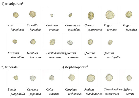
Figure 1.
Example pollen grain images used for analysis. The backgrounds of the images have been transparency-treated for easier viewing. 1 Pollen types (Morita ([26])).
2.2. Image Processing and Data Augmentation
The images used for analysis were taken as red–green–blue (RGB) color model images at 400× magnification with an image size of 1600 × 1200 pixels and resolution of 72 dots per inch (dpi), with a single pollen grain visible at the center of the image. Images were taken at five different levels, varying the focal point from the pollen surface closest to the objective lens (A in Figure 2) to that furthest away from the lens (E in Figure 2). Pollen from 100 individuals of each tree species was extracted and photographed at the five focal points to obtain 500 pollen images per tree species, for a total of 10,000 pollen images. For data augmentation, each image was rotated clockwise by 90°, 180°, or 270° to create four images from each photograph, or 2000 images per tree species, for a total of 40,000 images of 20 species with an image size of 1200 × 1200 pixels. The ImageJ software [30] was used for image processing, including image size conversion and rotation. The image size was set to 1200 × 1200 pixels because the deep learning model used in this study requires an image size of 256 × 256 pixels for training; however, the image size was automatically converted during training. Although deep learning algorithms can use various image sizes, in recent years, more algorithms have been developed to handle image sizes larger than 256 × 256 pixels; therefore, we retained the image size to the extent possible. Pollen images were captured using an optical microscope (BX51; Olympus, Tokyo, Japan) and a digital microscope camera (DP20; Olympus).
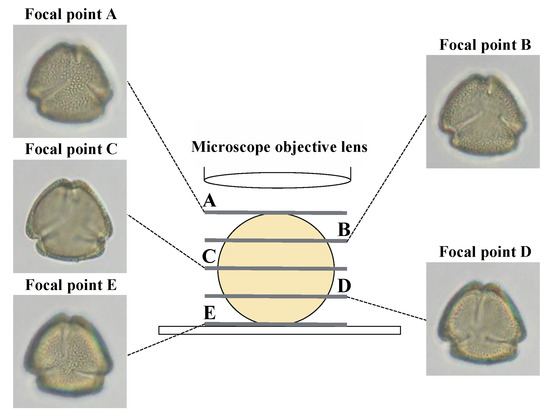
Figure 2.
Differences among captured images according to focal point position.
2.3. Learning Models, Learning Algorithms, and Learning Environment
CNNs are deep learning algorithms that are mainly composed of convolutional, pooling, and fully connected layers. The CNN model AlexNet exhibited vastly superior image identification accuracy at the 2012 ImageNet Large Scale Visual Recognition Challenge (ILSVRC) [31], which brought deep learning into the spotlight; since then, CNNs have become common in the field of image recognition. A CNN consists mainly of repeated convolution operations in the convolution and pooling layers, and then fully connected layers output the final processing results [13]. Among the various CNN algorithms, we used AlexNet and GoogLeNet, which were the winning models at ILSVRC in 2012 and 2014, respectively [32]. AlexNet consists of 11 layers: 5 convolutional layers, 3 max-pooling layers, and fully connected layers, with a linear layer with softmax activation at the output. GoogLeNet consists of 22 layers, including nine inception modules consisting of multiple convolution and pooling layers, and the ReLU activation function is applied to all convolution layers [32]. Both algorithms apply dropout regularization to overcome overfitting in the fully connected layers. The learning environment for the CNNs was a Linux operating system (Ubuntu 18.04 LTS), Intel CPU (Core i5-8400K), and GPU (NVIDIA GeForce RTX 2080 Super GPU) [33]. We used CUDA 11.6 and cuDNN 8.3.2 to support the GPU with deep learning. We used Caffe 0.17.3 (Convolutional Architecture for Fast Feature Embedding) as the learning framework for DIGITS 6.1.1 (NVIDIA deep learning GPU training system), which enables web-based learning. Caffe is a leading deep learning framework that supports numerous operating systems and has a rapid execution speed and hyperparameter tuning [34].
2.4. Simulation Conditions and Performance Evaluation
We divided pollen grain images into 10 equal sets, each of which included all 20 species. We devised four learning models, two patterns with and without data augmentation, and two patterns where the focal point image of the test data was the same as or different from the training data. The four learning models were as follows: Model 1 consisted of nine sets of training data and one set of test data, without data augmentation. Model 2 consisted of nine sets of training data and one set of test data, without data augmentation; however, as test data it used an image with a different focal point than the one used in the training data. Thus, if the training case had focal point A, the test data had focal points B–E. Model 3 was the same as Model 1 with data augmentation. Model 4 was the same as Model 2 with data augmentation. Models 3 and 4 with data augmentation were not divided into separate training and test datasets; i.e., the training and testing datasets were completely independent. The reasons for using different focal point images for the training and test data in Models 2 and 4 were as follows: We evaluated the effectiveness of the focal point images by comparing the classification accuracy of tree species identification at different focal points. If we had applied deep learning to various pollen grain images, the placement of the focal point in some of these images would have been unclear. Using images with different focal points allowed us to consider which types of images were desirable for use as training data, which may contribute to improving pollen grain images in the future. For all learning models, we conducted 10 model iterations without duplication. The average of the 10 simulation results was used in the analysis. We conducted 50, 100, and 200 epochs for all learning models. Thus, this study performed 360 simulations for Models 1 and 3 (360 = 6 focal point patterns (A through E, plus a dataset with all the focal points summarized) × 10 iterations × 2 data augmentations (with or without) for the training algorithm (AlexNet or GoogLeNet) × 3 epochs (50, 100 and 200)) and 1200 cases for Models 2 and 4 (1200 = 20 focal point patterns (5 focal points × 4) × 10 iterations × 2 data augmentations (with or without) the training algorithm (AlexNet or GoogLeNet) × 3 epochs (50, 100 and 200)).To evaluate the performance of the proposed models, we calculated the F score to quantify the classification accuracy of individual tree species, and the MCC, which measures overall classification accuracy [35,36,37]. In a classification model that uses contingency tables, TP is true positive, which is a correctly classified positive example; TN is true negative, which is a correctly classified negative example; FP is false positive, when the outcome is incorrectly predicted to be positive although it is actually negative; and FN is false negative, when the outcome is incorrectly predicted to be negative although it is actually positive. Equation (1) presents the precision (number of cases predicted to be positive that are actually positive), whereas Equation (2) presents the recall (the number of cases that were actually correct and predicted to be positive). Both are expressed as follows:
Both equations may be used as indices to evaluate the classification accuracy; however, they imply trade-offs [36,37]. We used the F score as an overall indicator; the F score is the harmonic mean of precision and recall, as follows:
The MCC indicates whether the classification is unbiased [35]. The MCC ranges from −1 to 1 and can be defined by a confusion matrix C for K classes [38], as follows:
where is the number of times class k actually occurred in the C of K,
is the number of times k was estimated in the C of K,
is the total number of samples correctly estimated, and
is the total number of samples [38].
3. Results
3.1. Tree Species Classification Accuracy for Test Data with Varying Focal Points
Table 2 shows the classification accuracy of tree species identification for test data with varying focal points. Among focal points without data augmentation, the highest MCC was 0.9070 (focal point D, AlexNet, 200 epochs), and the lowest MCC was 0.7486 (focal point D, GoogLeNet, 50 epochs). The difference between the maximum and minimum values for each focus point ranged from 0.0740 (focal point E) to 0.1584 (focal point D). Focal point D showed the largest variation among learning models, at approximately double that of focal point E. With the exception of two cases, classification accuracy tended to improve as the number of epochs increased. Among images with the same focal point and same number of epochs, classification accuracy tended to be higher with the AlexNet algorithm than with GoogLeNet, except in two cases. Among focal points with data augmentation, the highest MCC was 0.9286 for focal point E (GoogLeNet, 200 epochs), and the lowest MCC was 0.8274 for focal point A (AlexNet, 50 epochs). The difference between the maximum and minimum values at each focus ranged from 0.0579 (focal point C) to 0.0885 (focal point A), such that the overall variability was lower than without data augmentation. In seven cases, increasing the number of epochs decreased rather than improved the classification accuracy. Notably, the classification accuracy of focal points B, C, D, and E tended to decrease when the number of epochs in AlexNet increased from 100 to 200. Unlike our data augmentation results, for the same focal point and the same number of epochs, with data augmentation, GoogLeNet tended to yield higher classification accuracy than AlexNet. Using all data without data augmentation, the highest MCC was 0.9017 (AlexNet, 100 epochs), and the lowest MCC was 0.8182 (GoogLeNet, 50 epochs). GoogLeNet showed higher classification accuracy than the average value for focal points A–E with 50 epochs, whereas the average value showed higher accuracy as the number of epochs increased. For AlexNet, the MCC of all data was higher than the average value when the number of epochs was small, whereas the difference between the MCC of all data and that of the average value decreased as the number of epochs increased, and the MCC values were nearly equal at 200 epochs. When all data were used with data augmentation, the highest MCC was 0.9159 (GoogLeNet, 200 epochs), and the lowest MCC was 0.7844 (AlexNet, 50 epochs). For all data, GoogLeNet showed higher classification accuracy than the average value for focal points A–E at 200 epochs, whereas AlexNet showed higher accuracy at all epochs.
Table 2.
Tree species classification accuracy in terms of Matthews correlation coefficient (MCC), calculated from the sum of 10 simulation results. Numbers 1 and 2 indicate without and with data augmentation, respectively.
3.2. Tree Species Classification Accuracy for Images at Different Focal Points when Training Data Were Used as Test Data
Table 3 shows the tree species classification accuracy of the models for images at different focal points when training data were used as test data, with 200 epochs. We subtracted the MCC obtained when the training data were used as test data from that obtained when the training and test data consisted of different images (Diff). We also calculated the average of this value (Avg Diff), as well as the average difference calculated for each focal point image in each training model (Avg) and the average of this value (Overall Avg).
Table 3.
Tree species classification accuracy results for images taken at different focal points between the training and test data. The epoch number was 200 for all cases.
All Diff values were negative except for one case, suggesting that classification accuracy was decreased by using focal point images that were not included in the training data. The highest Diff value was −0.1939, and the lowest was −0.0010. Generally, Diff tended to increase as the distance between the focal points of the training and test images increased. If the focal points of the training and test images were adjacent (e.g., the focal point of a training image was B and that of the test image was A or C), then Diff was relatively small; however, when the focal points of the training and test images were separated by two or more points, Diff often reached large values, suggesting extremely low classification accuracy. Thus, focal point C, at the midpoint of our five focal points, resulted in the smallest decrease in classification accuracy when different focal point images were used as training and test data. By contrast, when the focal points of the training and test images were at opposite extremes of the range of five points, the lowest classification accuracy was obtained. For both GoogLeNet and AlexNet, Diff tended to be slightly larger with data augmentation than without data augmentation.
3.3. Tree Species Classification Accuracy according to Focal Points
Table S1 shows the variation in tree species classification accuracy results according to focal points. For focal point A, the highest F score was 0.995 (C.cr.) and the lowest was 0.545 (F.j.) without data augmentation, whereas the highest F score was 0.996 (C.cr.) and the lowest was 0.576 (C.t.) with data augmentation. The tree species that showed the highest and lowest F scores more than once (excluding averages) were C.cr., F.s., and Q.c. (without data augmentation) and C.co., C.t., and F.j. (with data augmentation), respectively. For focal point B, the highest F score was 0.995 (Q.c.) and the lowest was 0.619 (C.o.) without data augmentation, whereas the highest F score was 0.996 (Q.c.) and the lowest was 0.499 (C.o.) with data augmentation. Tree species showing the highest and lowest F scores more than once were C.cr. and Q.c. (without data augmentation) and C.co., Q.ser., and Q.ses. (with data augmentation), respectively. For focal point C, the highest F score was 0.990 (Q.c.) and the lowest was 0.470 (G.i.) without data augmentation, whereas the highest F score was 0.994 (C.cr.) and the lowest was 0.530 (C.co.) with data augmentation. Tree species showing the highest and lowest F scores more than once were C.cr., F.s., and Q.c. (without data augmentation) and C.co., G.i., Q.ser., and Q.ses. (with data augmentation), respectively. For focal point D, the highest F score was 0.980 (Q.c.) and the lowest was 0.209 (C.t.) without data augmentation, whereas the highest F score was 0.995 (C.cr.) and the lowest was 0.527 (G.i.) with data augmentation. Tree species showing the highest and lowest F scores more than once were F.s. and Q.c. (without data augmentation) and C.co., G.i., Q.ser., and Q.ses. (with data augmentation), respectively. For focal point E, the highest F score was 0.985 (Q.c.) and the lowest was 0.600 (C.co.) without data augmentation, whereas the highest F score was 0.991 (C.cr.) and the lowest was 0.591 (G.i.) with data augmentation. Tree species showing the highest and lowest F scores more than once were C.cr. and Q.c. (without data augmentation) and C.co., G.i., and Q.ser. (with data augmentation), respectively. For all data, the highest F score was 0.993 (Q.c.) and the lowest was 0.531 (G.i.) without data augmentation, whereas the highest F score was 0.992 (Q.c.) and the lowest was 0.370 (C.t.) with data augmentation. Tree species showing the highest and lowest F scores more than once were C.cr. and Q.c. (without data augmentation) and C.co., Q.ser., Q.ses., and C.t. (with data augmentation), respectively. Comparing the average values of the 20 tree species for each epoch showed that classification accuracy tended to improve as the number of epochs increased. However, when the number of epochs increased from 100 to 200, classification accuracy decreased slightly in some cases.
3.4. Misclassification Patterns according to Tree Species and Pollen Type
Based on the results presented in Table 2, we created heatmaps of the highest and lowest MCC values to visualize misclassification patterns according to tree species and pollen type, for models run with and without data augmentation, based on a contingency table of classification results for 10 simulations (Figure 3 and Figure 4). Figure 3 shows that all Q.c. and C.si. specimens were correctly classified, and C.cr. (1 total misclassification) and F.s. (2) specimens were almost all correctly classified. By contrast, species such as C.co. (19), F.c. (19), G.i. (18), Q.ser. (15), and Q.ses. (17) showed higher misclassification rates. The most commonly misclassified species were C.co. (9), Q.ser. (7), and F.c., G.i., and Q.ses. (5 each). Other tree species that were commonly misclassified as true positives were Q.ses. (8), Q.ser. (7), and A.j. and B.p. (6 each). We also found that F.c. (0) and C.cu. and J.m. (1 each) had low classification accuracy but were not frequently misclassified as positives. Among the most common misclassifications were Cam.j. to F.j. (8), G.i. to A.j. (8), Q.ses. to Q.ser. (8), and Z.s. to U.d. (8).
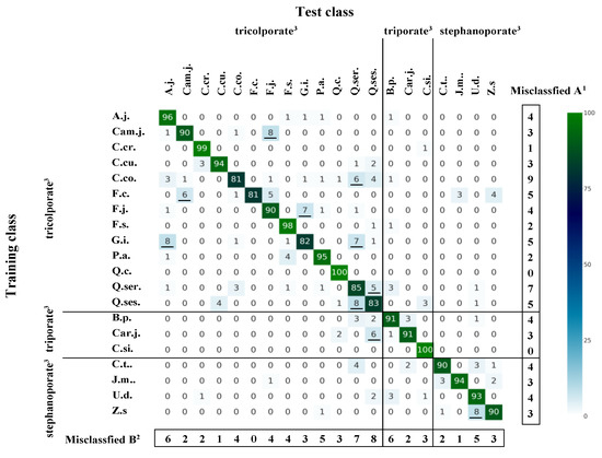
Figure 3.
Heatmap of misclassification patterns according to tree species and pollen type. Results were obtained using the AlexNet algorithm without data augmentation using focal point D and 200 epochs. Values are the sums of 10 simulation results. Underlining indicates the 10 most frequent cases. 1 Number of tree species misclassified, 2 number of times a species was misclassified as a positive example of another tree species, 3 pollen types (Morita [26]).
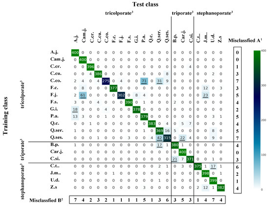
Figure 4.
Heatmap of misclassification patterns according to tree species and pollen type. Results were obtained using the GoogLeNet algorithm with data augmentation using focal point E and 200 epochs. Values are the sums of 10 simulation results. Underlining indicates the 10 most frequent cases. 1 Number of tree species misclassified, 2 number of times a species was misclassified as a positive example of another tree species, 3 pollen types (Morita [26]).
Figure 4 shows that A.j., Cam.j., and Car.j. were all correctly classified, and C.cr. (4), J.m. (2), and U.d. (1) were nearly always correctly classified. By contrast, species such as C.co. (125), F.j. (98), and Q.ses. (85) showed higher misclassification results. The most commonly misclassified species were C.co. and Q.ses. (7), C.t. (6), and F.j. and P.a. (5). Other tree species that were commonly misclassified as positives were A.j. and U.d. (7), Q.ses. (6), and P.a., Q.ser., and Car.j. (5 each). By contrast, although F.c., F.j., F.s., G.i., Q.c., and C.t. (1 each) had low classification accuracy, they were not frequently misclassified as positives. Among the most common misclassifications were C.co. to P.a. (71), F.j. for Cam.j. (61), Q.ses. for Q.ser. (42), and C.co. for Q.ser. (8).
Table 4 shows misclassification rates according to pollen type, normalized by the number of trees per pollen type, based on the results shown in Figure 3 and Figure 4. Based on the results shown in Figure 3 (without data augmentation, focal point D, AlexNet, 200 epochs), tricolporate and stephanoporate pollen grains were the pollen types least likely to be misidentified, whereas triporate pollen was the most frequently misidentified pollen type, and most often as tricolporate pollen. The tree species that were not misclassified when misclassified to different pollen types were Car.j. (triporate) and C.t. (stephanoporate) in the case of tricolporate, 10 species (tricolporate, except for Q.c., Q.ser., and Q.ses.) and 3 species (stephanoporate, except for U.d.) in the case of triporate, and 8 species (tricolporate, except for C.cr., F.j., P.a., Q.ser., and Q.ses.) in the case of stephanoporate.
Table 4.
Misclassification rates for each pollen type, normalized by the number of trees per pollen type.
Based on the results shown in Figure 4 (with data augmentation, focal point E, GoogLeNet, 200 epochs), triporate and stephanoporate were the pollen types least likely to be misidentified, whereas tricolporate was the most frequently misidentified pollen type, most often as triporate or stephanoporate pollen. The tree species that were not misclassified when misclassified to different pollen types were C.t. (stephanoporate) in the case of tricolporate, 10 species (tricolporate, except for A.j., Q.ser., and Q.ses.) and 3 species (stephanoporate, except for U.d.) in the case of triporate, and 9 species (tricolporate, except for F.c., P.a., Q.ser., and Q.ses.) and B.p. and C.si. (triporate) in the case of stephanoporate.
4. Discussion
Tree species classification accuracy was generally higher with data augmentation, and classification with focal point E showed the highest MCC value both with and without data augmentation (Table 2). Focal point D (AlexNet, 200 epochs) had the highest MCC value without data augmentation; however, MCC values were often lower for other focal points at low epoch numbers, and the lowest MCC values were obtained for average values. Without data augmentation, the focal point showing the highest classification accuracy differed among training models and epoch numbers, making it difficult to determine an optimal focal point. Conversely, with data augmentation, the classification accuracy of each focal point did not differ significantly among training models or epoch numbers, with focal point E showing the highest overall accuracy. Focal points E and A generally captured the surface structure of the pollen grains. We hypothesized that images where the focus is on the contour or membrane structure of the pollen grain (e.g., focal point C) would have higher classification accuracy than those where many features on the spherical grain are unclear (e.g., focal points B and D). However, the classification accuracy was not consistently lower for images taken with focal points B and D. Focal point C showed a slight tendency toward lower classification accuracy compared with the other focal points. Therefore, it appears that higher classification accuracy may be obtained when the focal point is closer to the pollen grain surface. Images that focused on the pollen surface tended to have higher classification accuracy, suggesting that differences in surface structure may have a significant effect; if this is the case, then misclassification should occur more frequently among species with similar pollen surface structures. For example, the pollen surfaces of F.s. and G.i. have a reticulate structure, whereas those of U.d. and Z.s. has a similar intricate, ridged structure. As shown in Figure 4, the most frequently misclassified species were C.cu. for F.s. (4 misclassifications, 0 for G.i.), A.j. for G.i. (18 misclassifications, 0 for F.s.), Q.ser. for U.d. (1 misclassification, 0 for Z.s.), and J.m. for Z.s. (12 misclassifications, 1 for Z.s.). Thus, we did not observe more misclassifications among tree species with similar pollen surface structures. Although species classification was not based on pollen surface structure alone, decisions based on images with a clear pollen surface structure were more accurate than those without such images.
Table 3 shows that tree species classification accuracy generally decreased when the focal point images differed between the training and test datasets, and that classification accuracy decreased as the distance increased between the focal points of the images used for training and testing. When images with different focal points were used for training and testing, there was less classification accuracy loss when focal point C was selected for the training data; therefore, it may be more effective to train data using an intermediate focal point when the focal point of the pollen grain image to be identified is unknown. However, focal point C tended to show lower classification accuracy than all other focal points; therefore, in accumulating a new pollen grain image dataset, it is appropriate to create images at focal point A or E, because these capture the pollen surface structure in a manner associated with high classification accuracy, and to apply a learning model created using images taken at focal point C to identify pollen grain images with unknown focal points.
In our previous studies on tree species identification by deep learning based on leaf images, GoogLeNet tended to show higher classification accuracy for most training patterns, regardless of whether data augmentation was applied [25,39,40]. In this study, GoogLeNet tended to have higher classification accuracy than AlexNet for many models. Due to similar results in tree species identification based on leaf images [12,41], GoogLeNet is regarded as one of the most effective deep learning algorithms. Since GoogLeNet has more layers than AlexNet, we consider that GoogLeNet can achieve higher discrimination accuracy. Many deep learning algorithms tend to improve classification performance when the number of layers is increased [13]. In this study, AlexNet showed higher classification accuracy than GoogLeNet in many cases, especially in learning without data augmentation. Progress has been made in developing deep learning algorithms with more convolutional and pooling layers, and models with more layers often have higher classification performance. Each deep learning algorithm has different constraints (image type and image size) on the input data for each algorithm. In particular, as the number of layers is increased, factors such as the method of combining layers, selection of activation functions to be applied, and adjustment of hyperparameters become more complex. Because it is not always clear which learning algorithm should be applied to the object to be identified in deep learning, it is necessary to consider various learning algorithms, and it is not always sufficient to select a model with a large number of layers. Furthermore, in many deep learning models, the learning time increases as the layer number increases, such that running various patterns (e.g., in this study, we varied the focal point and epoch number) can require enormous amounts of effort and time. Therefore, it is preferable to use a training model with as short a training time as possible and with high classification performance. As the AlexNet algorithm can be trained in less than half of the time required by GoogLeNet under the same training environment, we expect that AlexNet will be sufficient without data augmentation.
The classification accuracy of the training data also increased as the number of epochs increased, reaching almost 100% for most of the training models at an epoch number of 200. However, excessive learning can result in overfitting, which reduces classification accuracy [42]. In this study, when the epoch number was increased from 50 to 100, classification accuracy was greatly improved in some models, whereas when the epoch number was increased from 100 to 200, classification accuracy decreased slightly in some models, which may indicate overfitting.
As shown in Table S1, the classification accuracy results were generally similar to the tendency of misclassification patterns but differed slightly according to focal points. In this study, C.cr., F.s., and Q.c. showed the highest classification accuracy, whereas C.co., F.j., G.i., Q.ser., Q.ses., and C.t. showed the lowest classification accuracy. The results shown in Figure 3 (without data augmentation, focal point D, AlexNet, 200 epochs) were generally consistent with these results, although the trend varied depending on the learning model; A.j., Cam.j., C.cr., F.s., Q.c., and C.si. showed the highest classification accuracy, whereas C.co., F.j., G.i., and Q.ses. showed the lowest classification accuracy. Our results obtained without data augmentation cannot be used to interpret misclassification trends clearly due to the small number of overall data; however, based on our results with data augmentation (Figure 4), P.a. and Q.ser. were candidates for misclassification in many cases. Because we maintained a constant magnification level in this study, pollen grain size may have influenced these results. For example, C.cr. may have shown higher classification accuracy because its pollen grains are smaller than those of other tree species. However, our tree species classification accuracy results have not been verified in detail, and the issue of pollen size remains to be addressed in a future study.
Misclassification frequently occurred between species with the same pollen type (Figure 3 and Table 4). However, pollen grain misclassification rates were particularly high for certain tree species. For example, tricolporate was misidentified to Car.j. of triporate and C.t. of stephanoporate, triporate was misidentified to Q.c., Q.ser., and Q.ses. of tricolporate and U.d. of stephanoporate, and stephanoporate was misidentified to P.a., Q.ser. Q.ser., and Q.ses. of tricolporate and B.p. of triporate. In our previous studies on tree species identification using deep learning based on leaf images [39,40], these three groups were classified according to leaf morphological characteristics, and misclassification tended to occur most frequently (but not always) within the same group. However, as 100% identification is difficult, it is expected that even manual pollen identification can misclassify pollen grains among tree species with the same pollen type. Therefore, although it may be desirable to identify 100% of pollen grains to species, it is necessary to consider an evaluation method that assumes that misclassification will occur. For example, mean reciprocal ranking, which evaluates classified results in terms of probability and outputs them as ranks [41], may be effective for analyzing final classification results. Therefore, when constructing a practical identification system, it is necessary to consider several candidates in terms of the probability that the output matches the actual pollen grain, rather than presenting a single pollen grain type as the classified result.
Comparing our results with those of previous pollen identification studies using deep learning, we found F values of 0.967 [15], 0.963 [17], and 0.978 [18], which were higher than those reported in this study. However, these studies differed in various ways, including the implementation of a database of preprocessed pollen images; the application of fine-tuning [43], which is a method for re-training and adjusting parameters using weights from a model already trained on another image set; transfer learning [27], in which only the output layer is trained using hyperparameters from a trained model; or image preprocessing. Any of these methods could improve classification accuracy, such that our results cannot be compared directly with those of the cited studies.
5. Conclusions and Future Work
The objective of this study was to develop a deep learning-based tree species identification model using pollen grain images taken with a camera mounted on an optical microscope. Because pollen grains are roughly spherical, we evaluated the tree species classification accuracy of deep learning algorithms using images of the same pollen grains taken with different focal points. Although classification accuracy varied among tree species and it was difficult to identify all tree species without error, the best model showed an MCC value > 0.9 and was therefore found to have high accuracy. Future studies should evaluate learning models using pollen grains from more tree species and sedimentary fossil pollen and consider the application of other deep learning models. In this study, we verified the classification accuracy when the pollen analyst performs identification using various focal points, assuming that the material is actually used for pollen analysis. Since we focused on whether the materials used in this study could be identified, the deep learning model has not been fully verified. Currently, there are powerful networks, such as ResNet [44] and DenseNet [45], that have more layers than AlexNet or GoogLeNet. Generally, deep learning tends to upgrade image classification performance as the number of layers increases [13]. In addition, deep learning algorithms with many layers need a huge amount of computation as the number of layers increases, which causes long training times [43]. In addition, problems such as overfitting [42] and vanishing gradient problem [46] are also known. Therefore, it is preferable to consider the optimal type of learning model for different problem sets, rather than simply using a model with many layers. However, tree species identification was possible using deep learning from actual pollen data used in the pollen analysis. We believe that future validation using more powerful networks such as ResNet and DenseNet is necessary.
Supplementary Materials
The following supporting information can be downloaded at: https://www.mdpi.com/article/10.3390/app122412626/s1, Table S1: Tree species classification accuracy in terms of the F score for various focal points. Single and double underlining indicates minimum and maximum values, respectively, in terms of the number of epochs.
Author Contributions
Conceptualization, Y.M.; methodology, Y.M. and H.T.; software, Y.M.; validation, Y.M., K.S. and H.T.; formal analysis, Y.M. and K.S.; investigation, K.S.; resources, K.S. and H.T.; data curation, Y.M., K.S. and H.T.; writing—original draft preparation, Y.M. and K.S.; writing—review and editing, Y.M. and H.T.; visualization, Y.M.; supervision, Y.M.; project administration, Y.M. All authors have read and agreed to the published version of the manuscript.
Funding
This research received no external funding.
Institutional Review Board Statement
Not applicable.
Informed Consent Statement
Not applicable.
Data Availability Statement
Not applicable.
Acknowledgments
We thank the Forest Vegetation Dynamics Laboratory, Kyoto Prefectural University, and the collectors of specimens held in the laboratory, for allowing us to use their pollen samples in this study. Four anonymous referees provided valuable comments on earlier drafts of the manuscript.
Conflicts of Interest
The authors declare no conflict of interest.
Abbreviations
The following abbreviations are used in this manuscript:
| CNN | convolutional neural network |
| MCC | Matthews correlation coefficient |
| TP | true positive |
| TN | true negative |
| FP | false positive |
| FN | false negative |
| A.j. | Acer japonicum |
| B.p | Betula platyphylla |
| C.co. | Cornus controversa |
| C.cr. | Castanea crenata |
| C.cu. | Castanopsis cuspidata |
| C.si. | Celtis sinensis |
| C.t. | Carpinus tschonoskii |
| Cam.j. | |
| Car.j. | Carpinus japonica |
| F.j | Fagus japonica |
| F.c | Fagus crenata |
| F.s. | Fraxinus sieboldiana |
| G.i. | Gamblea innovans |
| J.m. | Juglans mandshurica |
| P.a. | Phellodendron amurense |
| Q.c | Quercus crispula |
| Q.ser | Quercus serrata |
| Q.ses | Quercus sessilifolia |
| U.d. | Ulmus davidiana var. japonica |
| Z.s. | Zelkova serrata |
References
- Nakamura, J. Pollen Analysis; Kokonsyoin: Tokyo, Japan, 1967. [Google Scholar]
- Stillman, E.; Flenley, J.R. The needs and prospects for automation in palynology. Quat. Sci. Rev. 1996, 15, 1–5. [Google Scholar] [CrossRef]
- Holt, K.A.; Bennett, K.D. Principles and methods for automated palynology. New Phytol. 2014, 203, 735–742. [Google Scholar] [CrossRef] [PubMed]
- Nakae, M.; Hosoya, T. Status survey of digitization of natural history collections in Japan. Jpn. Soc. Degit. Arch. 2019, 3, 345–349. [Google Scholar]
- GBIF Survey. 2015. Available online: https://science-net.kahaku.go.jp/contents/resource/GBIF_20151005_questionnaire.pdf (accessed on 21 April 2022).
- Li, P.; Flenley, J.R. Pollen texture identification using neural networks. Grana 1999, 38, 59–64. [Google Scholar] [CrossRef]
- Marcos, J.V.; Nava, R.; Cristóbal, G.; Redondo, R.; Escalante-Ramírez, B.; Bueno, G.; Dénizc, Ó.; González-Porto, A.; Pardoe, C.; Chung, F.; et al. Automated pollen identification using microscopic imaging and texture analysis. Micron 2015, 68, 36–46. [Google Scholar] [CrossRef]
- Daood, A.; Ribeiro, E.; Bush, M. Pollen recognition using a multi-layer hierarchical classifier. In Proceedings of the 2016 23rd International Conference on Pattern Recognition (ICPR), Cancun, Mexico, 4–8 December 2016; pp. 3091–3096. [Google Scholar]
- Gonçalves, A.B.; Souza, J.S.; da Silva, G.G.; Cereda, M.P.; Pott, A.; Naka, M.H.; Pistori, H. Feature extraction and machine learning for the classification of Brazilian Savannah pollen grains. PLoS ONE 2016, 11, e0157044. [Google Scholar] [CrossRef]
- France, I.; Duller, A.W.G.; Duller, G.A.T.; Lamb, H.F. A new approach to automated pollen analysis. Quat. Sci. Rev. 2000, 19, 537–546. [Google Scholar] [CrossRef]
- Takagi, M.; Shimoda, H. Handbook of Image Analysis—Revised Edition; University of Tokyo Press: Tokyo, Japan, 2004. [Google Scholar]
- Ghazi, M.M.; Yanikoglu, B.; Aptoula, E. Plant identification using deep neural networks via optimization of transfer learning parameters. Neurocomputing 2017, 235, 228–235. [Google Scholar] [CrossRef]
- Yamashita, T. An Illustrated Guide to Deep learning; Kodansha: Tokyo, Japan, 2016. [Google Scholar]
- Makino, K.; Nishizaki, H. Deep Learning to Begin with the Arithmetic and Raspberry Pi; CQ Shuppansha: Tokyo, Japan, 2018. [Google Scholar]
- Sevillano, V.; Aznarte, J.L. Improving classification of pollen grain images of the POLEN23E dataset through three different applications of deep learning convolutional neural networks. PLoS ONE 2018, 13, e0201807. [Google Scholar] [CrossRef]
- Gallardo-Caballero, R.; García-Orellana, C.J.; García-Manso, A.; González-Velasco, H.M.; Tormo-Molina, R.; Macías-Macías, M. Precise pollen grain detection in bright field microscopy using deep learning techniques. Sensors 2019, 19, 3583. [Google Scholar] [CrossRef]
- Mahbod, A.; Schaefer, G.; Exker, R.; Ellinger, I. Pollen grain microscopic image classification using an ensemble of fine-tuned deep convolutional neural networks. In Proceedings of the ICPR 2021: Pattern Recognition. ICPR International Workshops and Challenges, Virtual Event, 10–15 January 2021. [Google Scholar]
- Sevillano, V.; Holt, K.; Aznarte, J.L. Precise automatic classification of 46 different pollen types with convolutional neural networks. PLoS ONE 2020, 15, e0229751. [Google Scholar] [CrossRef] [PubMed]
- Kubera, E.; Kubik-Komar, A.; Piotrowska-Weryszko, K.; Skrzypiec, M. Deep learning methods for improving pollen monitoring. Sensors 2021, 21, 3526. [Google Scholar] [CrossRef] [PubMed]
- Boldeanu, M.; Cucu, H.; Burileanu, C.; Mărmureanu, L. Multi-input convolutional neural networks for automatic pollen classification. Appl. Sci. 2021, 11, 11707. [Google Scholar] [CrossRef]
- Ortega-Cisneros, S.; Ruiz-Varela, J.M.; Rivera-Acosta, M.A.; Rivera-Dominguez, J.; Moreno-Villalobos, P. Pollen grains classification with a deep learning system GPU-trained. IEEE Lat. Am. Trans. 2022, 20, 22–31. [Google Scholar] [CrossRef]
- Chen, X.; Ju, F. Automatic classification of pollen grain microscope images using a multi-scale classifier with SRGAN deblurring. Appl. Sci. 2022, 12, 7126. [Google Scholar] [CrossRef]
- POLEN23E. 2013. Available online: https://www.quantitative-plant.org/dataset/polen23e (accessed on 3 June 2022).
- Battiato, S.; Ortis, A.; Trenta, F.; Ascari, L.; Politi, M.; Siniscalco, N. POLLEN13K: A large scale microscope pollen grain image dataset. In Proceedings of the 2020 IEEE International Conference on Image Processing (ICIP), Abu Dhabi, United Arab Emirates, 25–28 October 2020. [Google Scholar]
- Minowa, Y.; Nagasaki, Y. Convolutional neural network applied to tree species identification based on leaf images. J. For. Plan. 2020, 26, 1–11. [Google Scholar] [CrossRef]
- Morita, Y. Classification, Morphological Categories, General Structure and Names of Pollen and Spores—Encyclopedia of Pollen Science; Asakurashoten: Tokyo, Japan, 1994. [Google Scholar]
- Shavlik, J. Transfer Learning. 2009. Available online: https://ftp.cs.wisc.edu/machine-learning/shavlik-group/torrey.handbook09.pdf (accessed on 25 August 2021).
- Perez, L.; Wang, J. The effectiveness of data augmentation in image classification using deep learning. arXiv 2017, arXiv:1712.04621. [Google Scholar]
- Faegri, K.; Iversen, J. Textbook of Pollen Analysis, 4th ed.; Faegri, K., Kaland, P.E., Krzywinski, K., Eds.; John Wiley & Sons Ltd.: New York, NY, USA, 1989. [Google Scholar]
- NIH. ImageJ. 2004. Available online: https://imagej.nih.gov/ij/ (accessed on 5 January 2022).
- Krizhevsky, A.; Sutskever, I.; Hinton, G.E. ImageNet classification with deep convolutional neural networks. Adv. Neural Inf. Process. Syst. 2012, 25, 1097–1105. [Google Scholar] [CrossRef]
- Szegedy, C.; Liu, W.; Jia, Y.; Sermanet, P.; Reed, S.; Anguelov, D.; Erhan, D.; Vanhoucke, V.; Rabinovich, A. Going deeper with convolutions. In Proceedings of the IEEE Conference on Computer Vision and Pattern Recognition, Boston, MA, USA, 7 June 2015; pp. 1–12. [Google Scholar]
- NVIDIA. 2016. Available online: https://developer.nvidia.com/cuda-toolkit/ (accessed on 5 January 2022).
- Jia, Y.; Shelhamer, E.; Donahue, J.; Karayev, S.; Long, J.; Girshick, R.; Guadarrama, S.; Darrell, T. Caffe: Convolutional architecture for fast feature embedding. In Proceedings of the 22nd ACM International Conference on Multimedia, Orlando, FL, USA, 3–7 November 2014; pp. 675–678. [Google Scholar]
- Matthews, B.W. Comparison of the predicted and observed secondary structure of T4 phage lysozyme. Biochim. Et Bio-phys. Acta (BBA)—Protein Struct. 1975, 405, 442–451. [Google Scholar] [CrossRef]
- Motoda, H.; Tsumoto, S.; Yamaguchi, T.; Numao, M. Fundamentals of Data Mining; Ohmsha: Tokyo, Japan, 2006. [Google Scholar]
- Witten, I.H.; Frank, E.; Hall, M.A. Data Mining, Practical Machine Learning Tools and Techniques, 3rd ed.; Morgan Kaufmann Publishers: Burlington, NJ, USA, 2011; pp. 163–180. [Google Scholar]
- Scikit-Learn. 2007. Available online: https://scikit-learn.org/stable/modules/model_evaluation.html#matthews-corrcoef (accessed on 5 February 2022).
- Minowa, Y.; Kubota, Y. Identification of broad-leaf trees using deep learning based on field photographs of multiple leaves. J. For. Res. 2022, 27, 246–254. [Google Scholar] [CrossRef]
- Minowa, Y.; Kubota, Y.; Nakatsukasa, S. Verification of a deep learning-based tree species identification model using images of broadleaf and coniferous tree leaves. Forests. 2022, 13, 943. [Google Scholar] [CrossRef]
- Goëau, H.; Bonnet, P.; Joly, A. LifeCLEF plant identification task 2015. CLEF (Working Notes). In Proceedings of the Working Notes for CLEF 2014 Conference, Sheffield, UK, 15–18 September 2014. [Google Scholar]
- Raschka, S.; Mirjalili, V. Python Machine Learning Programming; Impress: Tokyo, Japan, 2018. (In Japanese) [Google Scholar]
- Li, Z.; Hoiem, D. Learning without forgetting. IEEE Trans. Pattern Anal. Mach. Intell. 2017, 40, 2935–2947. [Google Scholar] [CrossRef] [PubMed]
- He, Z.; Zhang, Z.; Ren, S.; Sun, J. Deep residual learning for image recognition. In Proceedings of the Proceedings of the IEEE Conference on Computer Vision and Pattern Recognition, Boston, MA, USA, 7–12 June 2015. [Google Scholar]
- Huang, G.; Liu, Z.; Maaten, L.; Weinberger, K.Q. Densely connected convolutional networks. In Proceedings of the Proceedings of the IEEE Conference on Computer Vision and Pattern Recognition, Las Vegas, NV, USA, 27–30 June 2016. [Google Scholar]
- Okatani, T. On deep learning. J. Robotics. Soc. Jpn. 2015, 33, 92–96. [Google Scholar] [CrossRef]
Publisher’s Note: MDPI stays neutral with regard to jurisdictional claims in published maps and institutional affiliations. |
© 2022 by the authors. Licensee MDPI, Basel, Switzerland. This article is an open access article distributed under the terms and conditions of the Creative Commons Attribution (CC BY) license (https://creativecommons.org/licenses/by/4.0/).