Article

Multi-Objective Antenna Design Based on BP Neural Network Surrogate Model Optimized by Improved Sparrow Search Algorithm

School of Electronic and Communication Engineering, Guangzhou University, Guangzhou 510006, China
*
Author to whom correspondence should be addressed.
Appl. Sci. 2022, 12(24), 12543; https://doi.org/10.3390/app122412543
Submission received: 26 October 2022 / Revised: 2 December 2022 / Accepted: 5 December 2022 / Published: 7 December 2022
(This article belongs to the Topic Artificial Intelligence Models, Tools and Applications)

Abstract

:
To solve the time-consuming, laborious, and inefficient problems of traditional methods using classical optimization algorithms combined with electromagnetic simulation software to design antennas, an efficient design method of the multi-objective antenna is proposed based on the multi-strategy improved sparrow search algorithm (MISSA) to optimize a BP neural network. Three strategies, namely Bernoulli chaotic mapping, inertial weights, and t-distribution, are introduced into the sparrow search algorithm to improve its convergent speed and accuracy. Using the Bernoulli chaotic map to process the population of sparrows to enhance its population richness, the weight is introduced into the updated position of the sparrow to improve its search ability. The adaptive t-distribution is used to interfere and mutate some individual sparrows to make the algorithm reach the optimal solution more quickly. The initial parameters of the BP neural network were optimized using the improved sparrow search algorithm to obtain the optimized MISSA-BP antenna surrogate model. This model is combined with multi-objective particle swarm optimization (MOPSO) to solve the design problem of the multi-objective antenna and verified by a triple-frequency antenna. The simulated results show that this method can predict the performance of the antennas more accurately and can also design the multi-objective antenna that meets the requirements. The practicality of the method is further verified by producing a real antenna.

1. Introduction

Antennas are indispensable devices in modern life and are widely used in radio communications, radar, and navigation. With the diversification of antenna applications, some antennas must simultaneously satisfy more than one objective. The structure of the antennas is more complicated than before and designing the antenna has become a challenging problem [1,2,3]. Currently, the traditional design process of antenna optimization usually requires applying electromagnetic simulation software, which can accurately evaluate the antenna’s performance, such as return loss and gain. The accuracy of the electromagnetic simulation is high. However, it has some problems, such as extensive calculations and time-consuming [4].
To address the defects of traditional methods, some scholars have begun to study new methods of antenna design. That is to use the surrogate model to replace standard simulation software. This method builds a nonlinear relationship between the size and performance of the antenna, making the antenna design more efficient and less complicated. The surrogate models commonly used in antenna design include support vector regression (SVR) [5,6], kriging model (KM) [7,8,9], and artificial neural network (ANN) [10,11,12,13,14,15,16], etc. Literature [5,6] constructed a surrogate model based on support vector regression (SVR). However, when experimental data are small, it will lead to inaccurate modeling and some errors in predicting antenna performance. Literature [7,8,9] used the Kriging algorithm to construct surrogate models for the antenna design. This method is a random interpolation method based on the general least-square way, and the prediction accuracy of data with large fluctuations needs further improvement.
Artificial neural networks represent structures created by neural nodes capable of establishing a nonlinear relationship between input and output data to predict the input data. This solid nonlinear prediction ability also makes artificial neural network surrogate models widely used in antenna design. Classical artificial neural networks include multi-layer perception (MLP) [10,11], radial basis function (RBF) [12,13], and BP neural networks (BPNN) [14,15,16]. However, BPNN has the benefits of self-learning capability, time-saving calculation, and strong generalization ability [16], and it has been widely used in many fields. Gao, Y. [14] used BPNN to build the state of charge (SOC) estimated model of the electric vehicle battery, and the feedback of BPNN was used to correct the error. And the average error of the estimated model is less than 0.5%. Hu, W. [15] proposed a BPNN steering angle prediction method to obtain the front wheel’s steering angle. The results show that the mean square error is less than 0.66, indicating that the method works well. Dong, J. [16] optimized the structure of BPNN because of its redundant connection and a lot of calculations, built the surrogate model based on l1-BPNN, and improved the efficiency of antenna design.
Although BPNN has achieved good results in different areas, there are still some drawbacks. The structural parameters determine its output. Usually, using random parameters will make the neural network unstable, and it is not easy to achieve the global optimum during optimization, resulting in insufficient prediction accuracy [17,18,19]. This requires optimizing its parameters, such as adding a dynamic learning rate to the original BP algorithm to correct the deficiency and enhance the prediction performance [20]. However, this gradient-based algorithm has limitations in global search capability [21]. In recent years, the emergence of intelligent bionic algorithms has overcome this limitation. For example, the sparrow search algorithm [22] is a relatively novel intelligent algorithm discovered by Xue. It has the characteristics of less variable parameters, strong stability, simple operation, and strong global searchability. It performs well in optimizing the parameters of BPNN. In the literature [23], the sparrow search algorithm (SSA) and particle swarm algorithm (PSO) are used to optimize BPNN, and the experiments show that the model of SSA-BPNN has higher accuracy for the prediction and classification of water sources. In reference [24], tent chaotic map is introduced to improve SSA, which is used to optimize BPNN. After optimization, the number of iterations of the model is reduced by 75%, and the predicted value is more accurate.
However, in the late stage of solving complex optimization problems, SSA has a slow convergent speed and reduces the population’s diversity, making optimizing the situation challenging. Given the existing problems of SSA, many scholars have conducted in-depth research on it. Nguyen et al. [25] used a reverse learning method to dispose of the problems of the population and added the firefly algorithm to improve the exploration capability of the algorithm. Wu et al. [26] introduced a greedy algorithm to deal with the shortage of the population and then used the strategies of genetic operators and sine-cosine search to update the population and searchers to augment the robustness of SSA. Yan et al. [27] proposed a variable helical factor strategy and a local iterative search strategy. At the same time, it improved the control of boundary, which improved the problem of low accuracy in the SSA search process and the convergent accuracy. L. Jianhua et al. [28] introduced the chaos map to enhance the singleness of the population. They used “dispersion” to update the search rules so that the algorithm could reach the ideal target solution faster. Although the above scholars have proposed some improvements to SSA, which have enhanced some of the capabilities of the algorithm, effective strategies are still needed to improve the initialization of the population and convergent accuracy.
For the above reasons, this paper proposes a multi-strategy improved sparrow algorithm (MISSA) to improve the shortcomings of BPNN. The optimized BPNN has a stronger ability for prediction. First, the Bernoulli chaotic map draws in the sparrow population to address the lack of abundance of the primitive population. In the meantime, the inertia weight of the finder’s position update equation strengthens the capability of search and increases its performance. Finally, the adaptive t- distribution is added. The distribution interferes with the individual, so the algorithm is more active when searching and reaches the ideal target value. The effectiveness of MISSA is verified by comparing MISSA with the particle swarm algorithm (PSO) [29], grey wolf algorithm (GWO) [30], whale optimization algorithm (WOA) [31], and SSA on ten benchmark functions for optimal performance. The improved MISSA-BP surrogate model has better performance than others. Meanwhile, the design case of the microstrip antenna also confirms the practicality and efficiency of the method in the paper.
The other parts of this article are as follows. Section 2 describes the problem of designing the multi-objective antenna. Section 3 introduces the sparrow search algorithm and its improved strategies. Section 4 describes the constructed surrogate model based on MISSA-BP and the design method for multi-objective antennas based on this model. Section 5 utilizes the benchmark function to test the performance of the improved sparrow search algorithm and uses a design example of a planar microstrip antenna to verify the availability of the proposed method. Section 6 summarizes the content of this paper.

2. Problem Description

The following equation can express the problem of optimizing the multi-objective of the antenna:
min   F ( x ) = [ f 1 ( x ) , f 2 ( x ) , , f n ( x ) ] T s . t .   x X             X R m
In the equation, a design variable x = [ x 1 , x 2 , , x m ] T X R m is a group of determined vectors. It represents m structural sizes of the antenna that need to be processed in this paper. X is the space of parameters that is decided by the boundary of the structural parameters of the antenna. f j ( x ) , ( j = 1 , 2 , , n ) are n objective functions to be optimized. The main objective of antenna design is to reduce the reflection coefficient of a specific frequency band. Still, other indicators of the antenna have high demands in many cases. The different indicators will have clashed, making it difficult to reach the optimal solution simultaneously. At this time, we demand an answer in the middle to solve the problem, which is called the non-dominated solution set. All solutions in the non-dominated solution set constitute the Pareto front (PF) [32]. In this paper, PF is the solution we need to get. PF represents the intermediate answer to the multi-objective antenna, and we can design the antenna according to it.

3. Improved Sparrow Search Algorithm

3.1. Sparrow Search Algorithm

The sparrow search algorithm is a bionic intelligent algorithm proposed based on the influence of two different behaviors of sparrows in the process of finding food. It is more advantageous than existing algorithms in operational accuracy and global optimization. Sparrows are separated into two groups when looking for food: the finder and the follower. In SSA, the top-ranked part of fitness is the finder. The finders need to find the food and share the information about the food with all sparrows. The remaining sparrows will need to follow the directions of the finder to forage for food. For one thing, followers will plunder resources to find more food for themselves when the finders find an area rich in resources. For another, when a part of the sparrow is alerted to danger, it will send a cautionary message and quickly move to safe places to avoid predatory behavior.
Supposing there are N sparrows in d-dimensional space, each sparrow’s position and fitness value are X = [ x 1 , x 2 , , x D ] and F = f [ x 1 , x 2 , , x D ] . The SSA consists of three core parts, which will be introduced in the following paragraphs.
In the SSA, the finders must seek food and direct the followers’ behavior. The location of the finder is updated as below:
X m , d t + 1 = X m , d t exp ( m α T ) , R 2 < S T X m . d t + Q L , R 2   S T
where X m , d means the location information; t + 1 represents the present evolutionary algebra; T denotes the maximal evolutionary algebra; Both α and Q are uncertain figures, where is α between (0, 1] and Q is distributed according to N(0, 1); L is an array with 1 row and D columns, the value of each column is 1; R 2 represents the alert value, which is a numerical value between [0, 1]; S T expresses a secure value between [0.5, 1]. While R 2 < S T , it means that there is no danger nearby at this time, so the sparrows with higher fitness can get a supply of more prosperous food. In addition to this case, it indicates that some sparrows sense dangerous signals and give a warning, while the rest will go to new places to look for food.
The updated equation of the follower’s position is as follows:
X m , d t + 1 = Q exp ( X worst t X m , d t m 2 ) , m > n 2 X best t + 1 + X m , d t X best t + 1 A + L , m n 2
where X b e s t t + 1 and X w o r s t t represent the contrary meaning, indicating the best and worst information of position at the corresponding evolution times. A is a matrix with 1 row and d columns, all elements are ± 1 , and the condition A + = A T ( A A T ) 1 is satisfied. When m > n / 2 the mth individual with poor fitness can’t find food, they must go to a new place to find food; in another case, it represents that the mth sparrow is foraging near the ideal position.
Some sparrows are in charge of surveillance, alerting remaining individuals when danger is found approaching. The number of early-warning sparrows is usually slightly more than one-tenth of the population. The mathematical expression is as follows:
X m , d t + 1 = X best t + β ( X m , d t X best t ) , f m f g X m , d t + K ( X m , d t X w o r s t t f m f w + e ) , f m = f g
where β and K both are random numbers, where β is a random number according to N(0,1), representing the step size; K is within [−1,1]. e is an infinitely small number, preventing the dividend from being meaningless. When f m f g , it means some individuals are about to leave the range of food seeking, and the danger is serious. If f m = f g , this indicates that some individuals near the middle position have been aware of the threat, and this population of the sparrows must avoid risk and move to the safe place.

3.2. Improved Strategies

3.2.1. Chaos Mapping Strategy

Chaos is a common phenomenon in nonlinear systems. It is often applied to intelligent swarm optimization algorithms due to pseudo-random and ergodic characteristics [33]. Since the population of the sparrow is randomly generated when SSA is initialized, it will cause problems, such as reduced diversity of the population and low convergent accuracy in the later stage of solving complex optimization problems. Therefore, using chaotic mapping to process the population can achieve better results, and this is also commonly used in algorithms. The widely used chaotic mappings include logistic mapping, tent mapping, Bernoulli mapping, etc. The distribution histograms of the three mappings are shown in Figure 1. From Figure 1, it can be known that the distribution of logistic mapping values in the range of [0, 0.1] and [0.9, 1] is relatively large. That is, the density of the mapping points on both sides is high, and the density in the middle is low, reducing the operational speed and other indicators of performance. Although the distribution of tent mapping is more uniform than that of logistic mapping, and the convergent speed is faster, tent mapping has irregular periods and is prone to problems at fixed points. The distribution of Bernoulli mapping values is more uniform. There will be no problems at fixed points, and the convergent speed is faster. Therefore, Bernoulli mapping is applied in SSA to deal with the defects of the population in this paper. The expression of Bernoulli mapping is as follows:
Z k + 1 = Z k / ( 1 λ ) , Z k ( 0 , 1 λ ]   ( Z k 1 + λ ) / λ , Z k ( 1 λ , 1 ]  

3.2.2. Weight Strategy

It can be seen from Equation (2) that when R 2 S T , the finder will move according to the distribution set by the algorithm. Its value will converge to the ideal value. If R 2 < S T , the change of the finder’s position is not excellent, the equation is as follows:
y = exp ( x α T )
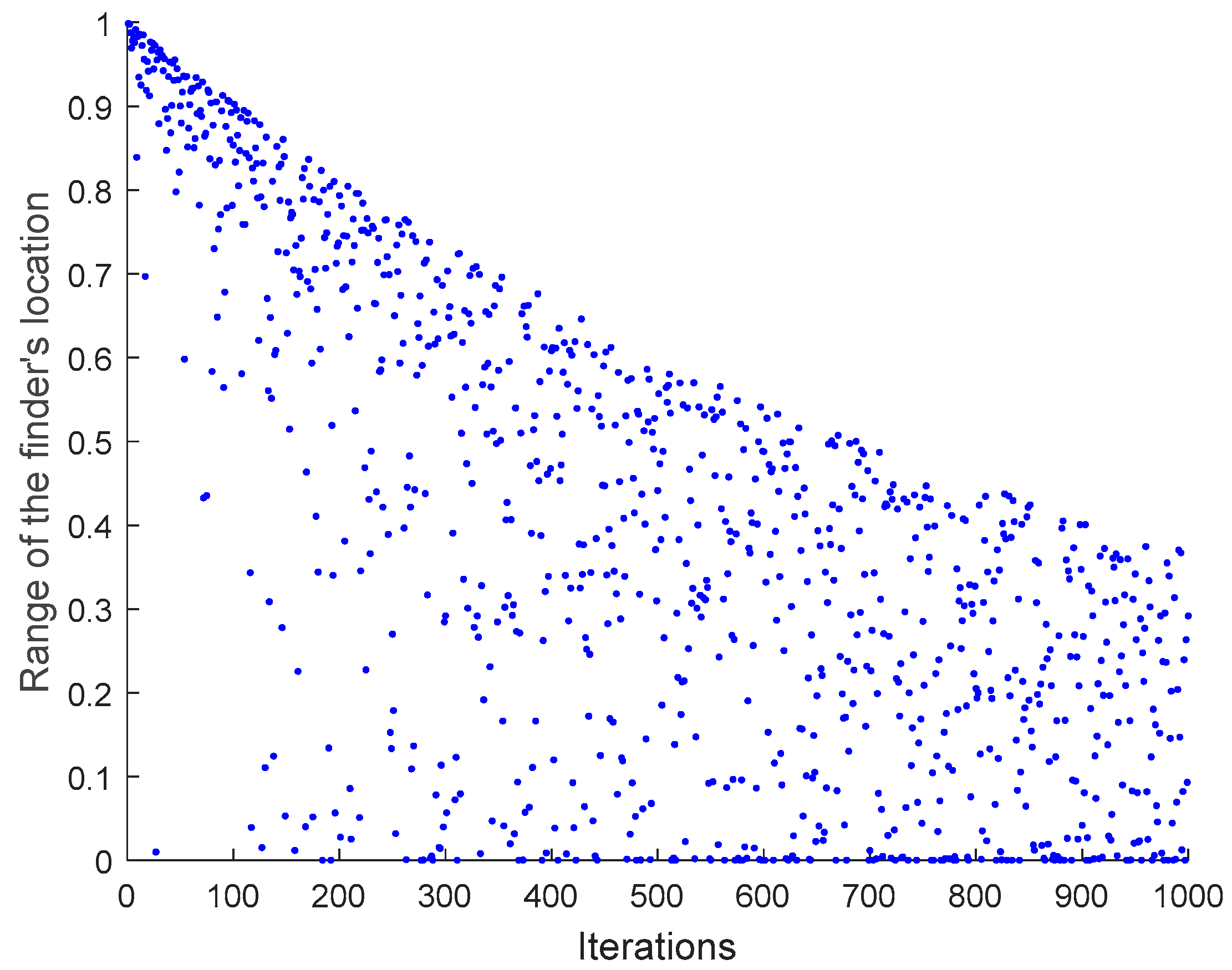
where x means the current number of evolutions, T is an upper evolutionary threshold set by the algorithm, and y is the variation range of the finder’s location. When T is 1000, the image of Equation (6) is shown in Figure 2.
Figure 2 shows the change in the location of the finder. As x increases, y gradually decreases, and its value range becomes (0, 0.4). When x approaches 0, the distribution of y is uneven, and the probability of nearly 1 is high. As x increases, y shows a uniform distribution. Therefore, when R 2 < S T , the variation range of individuals in the algorithm becomes smaller and smaller and gradually approaches 0. This search strategy enhances the local search ability of SSA. However, it is hard to achieve the desired value in later iterations.
To further improve the optimization performance of SSA, adaptive inertia weight is added to the updated equation of the finder’s position. The new updated equation is as follows:
X m , d t + 1 = X m , d t exp ( m w α T ) , R 2 < S T X m . d t + Q L , R 2   S T
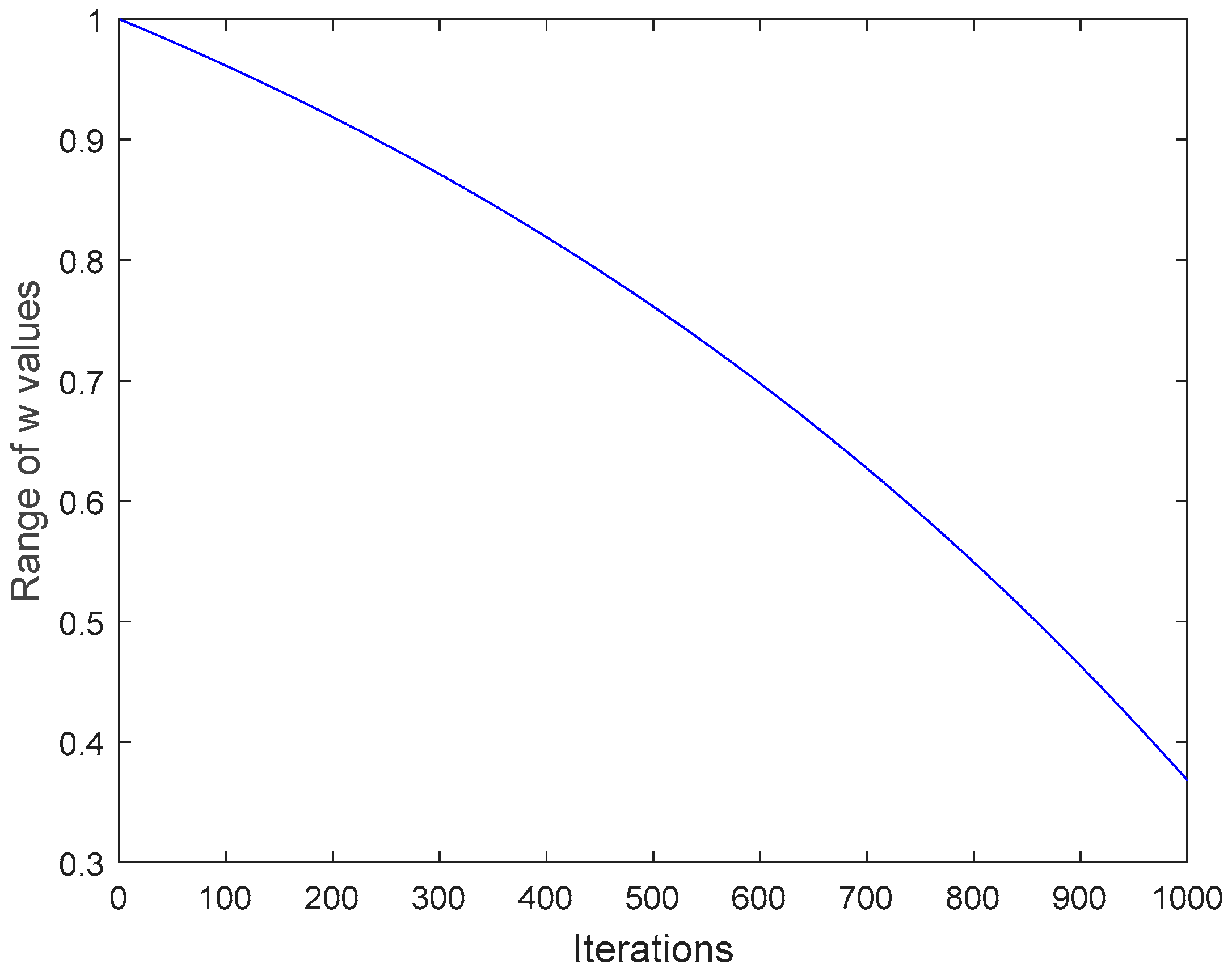
where   w = 1 exp ( t / T ) 1 exp ( 1 )
where w is an adaptive inertia weight, its value will gradually decrease along with t increases. Figure 3 indicates its image features. One knows that its value is relatively large in the early stage of the iteration of w, i.e., the initial algorithm will perform a large-scale search. When the t in the algorithm changes by adding 1, the value of w gradually decreases, strengthening SSA’s partial performance in the later stage of evolution, such as convergent accuracy.

3.2.3. Adaptive t-Distribution Strategy

In the later stage of SSA iteration, sparrows will move nearer to the optimum individual step by step. This leads to a decrease in the number of sparrows, and the algorithm may converge prematurely. This paper introduces adaptive t-distribution to optimize SSA to solve this problem. The t-distribution, Cauchy distribution, and Gaussian distribution are classical distributions in mathematics. The t-distribution is a particular distribution that can be converted between the Cauchy distribution and the Gaussian distribution, and it only needs to change its parameter n. When n = 1, the t-distribution is identical to the Cauchy distribution C (0, 1), and when n ≥ 30, the t-distribution is equivalent to the Gaussian distribution N (0, 1) [34]. The update equation for the location changes of sparrows using this strategy is described as below:
X m t + 1 = X m t + X m t t ( i t e r )
where   t ( i t e r ) = G a m i t e r + 1 2 i t e r π G a m i t e r 2 1 + x 2 i t e r i t e r + 1 2 ,   < x <
where X m t + 1 stands for the new location information of the mth sparrow after t-distribution variation, and X m t means the location information of the mth sparrow in the tth generation. t ( i t e r ) is a t-distribution, and its degrees of freedom is the number of iterations of the SSA. Gam(x) is the Gamma function.
The mutational update equation first uses the sparrow’s position in the current period. It adds the disturbance of the adaptive t-distribution, and its degree of freedom changes with the iteration of SSA. In the early stage of iteration, the t-distribution is similar to the Cauchy distribution, and the global search ability is improved. In the late iteration of SSA, the t- distribution becomes a Gaussian distribution, and the part search capability of the algorithm is enhanced at this time, which can make the convergent accuracy more accurate.

3.3. Improved Sparrow Search Algorithm

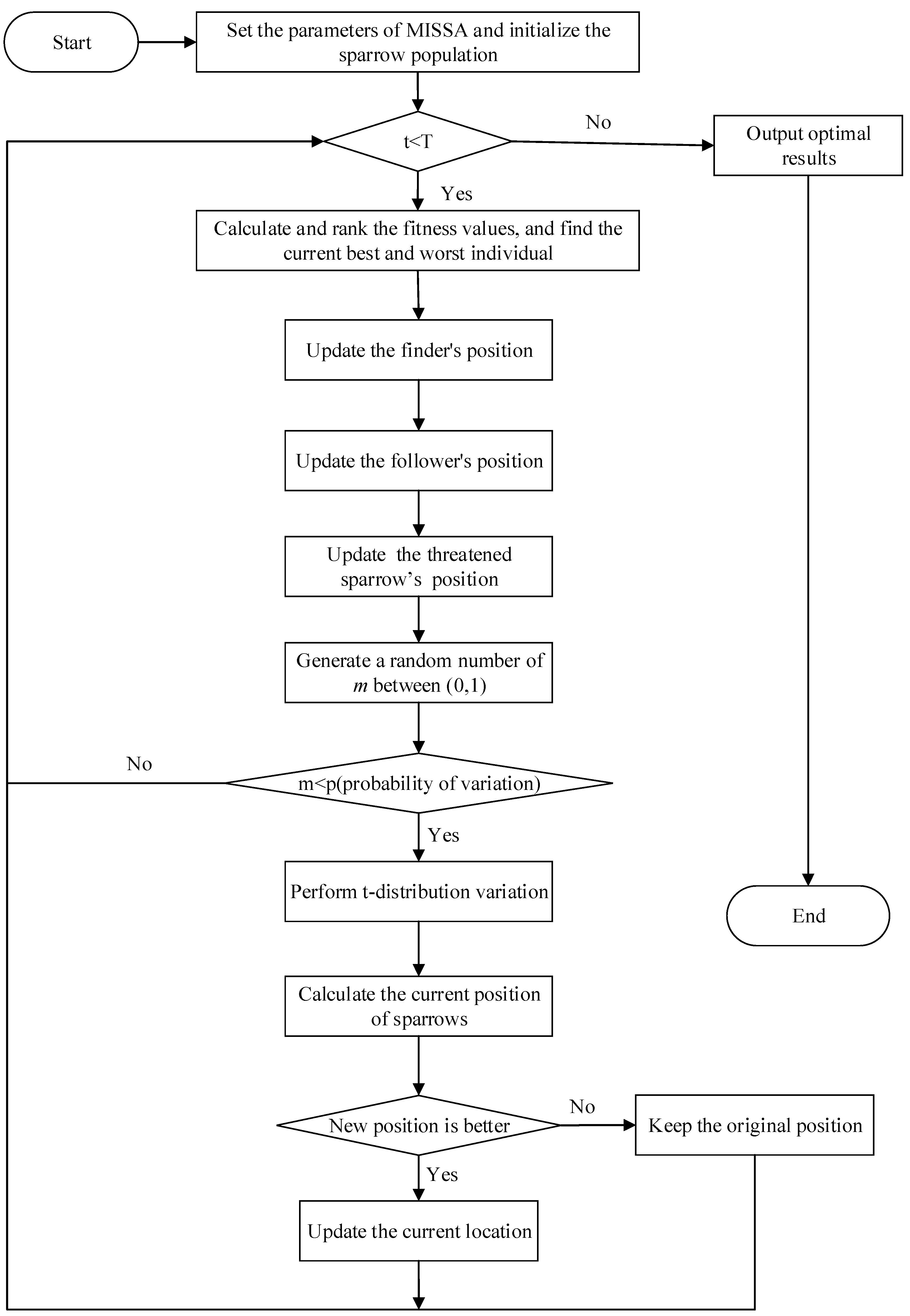
The above three strategies are introduced to improve the sparrow search algorithm so that the diversity of the population of SSA is improved, and the search method is improved to optimize the performance. The experimental results are presented in Section 5. Figure 4 is the flowsheet of the MISSA proposed in this paper, and the implementation procedure of MISSA is illustrated in Algorithm 1.
Algorithm 1: The framework of MISSA.
/* Initialization */
1. Set the maximum number of evolutions as T;
2. Set the population number of sparrows as n;
3. Set the warning value as ST;
4. Set the number of finders as PD;
5. Set the number of threatened sparrows as SD;
6. Set the variation probability of t distribution as p;
7. Initialize the population of sparrows using Equation (5);
/* Iterative optimization */
8. while (t < T)
9. Calculate and rank the fitness values, and find the current best and worst individual;
10. ST = rand (1)
11. for I = 1: PD
12. Use Equation (7) to update the finder’s position;
13. end for
14. for i = (PD + 1): n
15. Use Equation (3) to update the follower’s position;
16. end for
17. for i = 1:SD
18. Use Equation (4) to update the threatened sparrow’s position;
19. end for
20. Generate a random number of m between (0,1);
21. If m < p, use Equation (9) to conduct interference variation on sparrow individuals;
22. Calculate the current new position;
23. If the new position is better than before, update it;
24. t = t + 1;
25. end while
26. Output the best solution

4. Multi-Objective Antenna Design Method

4.1. MISSA-BP Surrogate Model

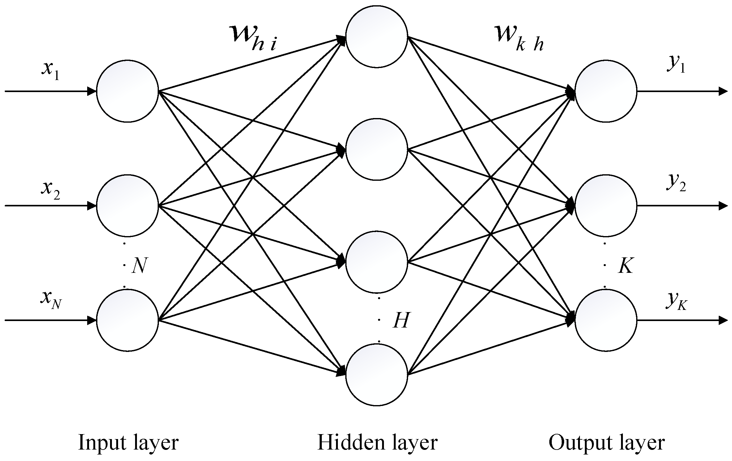
The BP neural network is a multi-layer network developed from MLP, with forwarding propagation of inputs and backward propagation of obtained errors. Owing to BP neural network’s low computational cost and strong generalization ability, it has been favored by many scholars [35]. The BP neural network comprises three layers: the input layer, the output layer, and the hidden layer. The number of nodes in each layer is designed according to the actual problem, and its brief structure is shown in Figure 5. It follows that the output of the network is calculated as follows:
I h = f 1 ( i = 1 N w h i x i + θ h )
y k = f 2 ( h = 1 H w k h I h + θ k )
where w h i and w k h indicate the weight connecting two different nodes; θ h and θ k correspond to the threshold of hidden layer and output layer; f 1 and f 2 are activation functions of corresponding layers of BP neural network.
It can be seen from Equations (11) and (12) that some parameters of the neural network determine the desired result y k that we want. Usually, using random parameters will make the neural network unstable, and it is laborious to achieve the ideal objective during optimization, resulting in insufficient accuracy of prediction. In this paper, MISSA is used to deal with the problems of the traditional neural network to improve its performance. MISSA will optimize the initial parameters, and the results will be output when the number of iterations is reached. The MISSA-BP surrogate model is obtained by substituting these optimized parameters into the neural network.

4.2. Multi-Objective Antenna Design Scheme Based on MISSA-BP

In this paper, the antenna surrogate model based on MISSA-BP is linked to the multi-objective particle swarm optimization (MOPSO) [36] to design a multi-objective antenna. MOPSO has fewer parameters and faster convergence compared to other multi-objective algorithms. It can also obtain the set of solutions covering the whole search space and close to the actual Pareto front with as few computational resources as possible. Each particle in MOPSO consists of n-size parameters in the antenna to be optimized; that is, each particle represents the structure of an antenna. By iterative search, when the end of the condition is reached, the result can be output to get the antenna that meets the requirement.
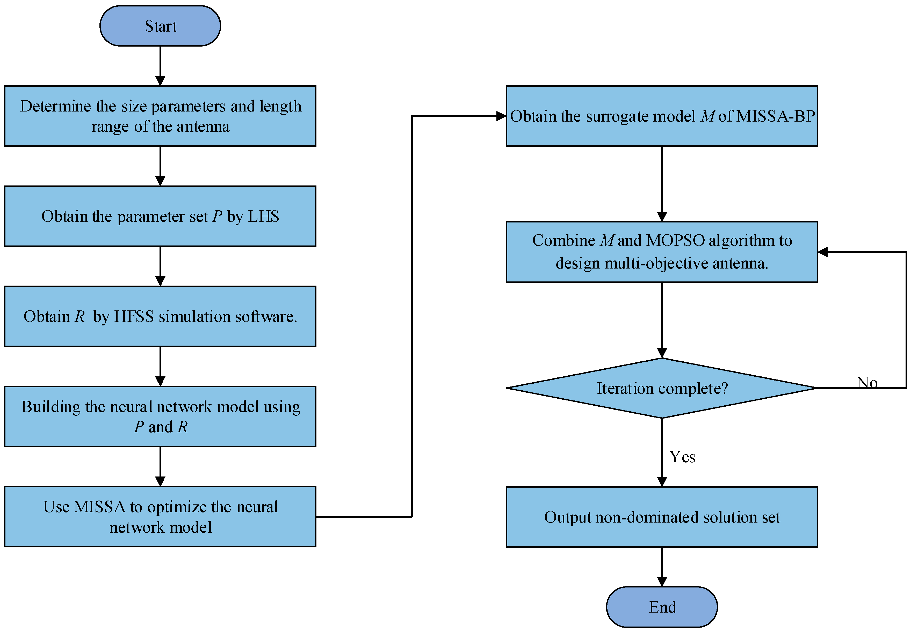
Figure 6 is the design flow chart of the multi-objective antenna based on MISSA-BP. The specific steps are as follows:
  • Step 1. Determining the size parameters and length range of the antenna.
  • Step 2. Latin hypercube sampling (LHS) is used for uniform sampling within the length range of the antenna, and the parameter set P is obtained.
  • Step 3. Substituting P into HFSS simulation software to obtain result set R.
  • Step 4. Building the neural network model using P and R.
  • Step 5. Using MISSA to optimize the parameters of the neural network, the surrogate model M of MISSA-BP is obtained.
  • Step 6. Combine M and the MOPSO algorithm to design the multi-objective antenna.
  • Step 7. If the iteration is not completed, continue to step 5. Otherwise, end the optimization and output the non-dominated solution set.

5. Simulation and Verification

5.1. Verification of MISSA

To verify the accuracy and efficiency of the MISSA, PSO, GWO, WOA, and the original SSA were added to the test to compare with it. The specific information of the ten classic benchmark functions is shown in Table 1. The first five are unimodal, and the last five are multimodal. The experiments were carried out in the same simulation environment. The computer used is an Intel Core i7-10700 processor, 2.90 GHz, 16G RAM, Windows 10 system, and the simulation software is MATLAB R2020b and Ansys HFSS 2021 R1.
PSO parameter setting: c1 = 1.6, c2 = 1.4, w = 0.75; GWO parameter setting: optimal solution a is between [0, 2]; WOA parameter setting: a = 0, b = 1; SSA and MISSA parameter setting: ST = 0.85, PD = 0.18, SD = 0.18. At the same time, the upper iteration limit of all algorithms is T = 500, and the number of the population is N = 30.
The five algorithms are tested on every function for 30 cycles to avoid randomness, and the corresponding results are taken. Table 2 records the relevant indicators corresponding to the algorithm.
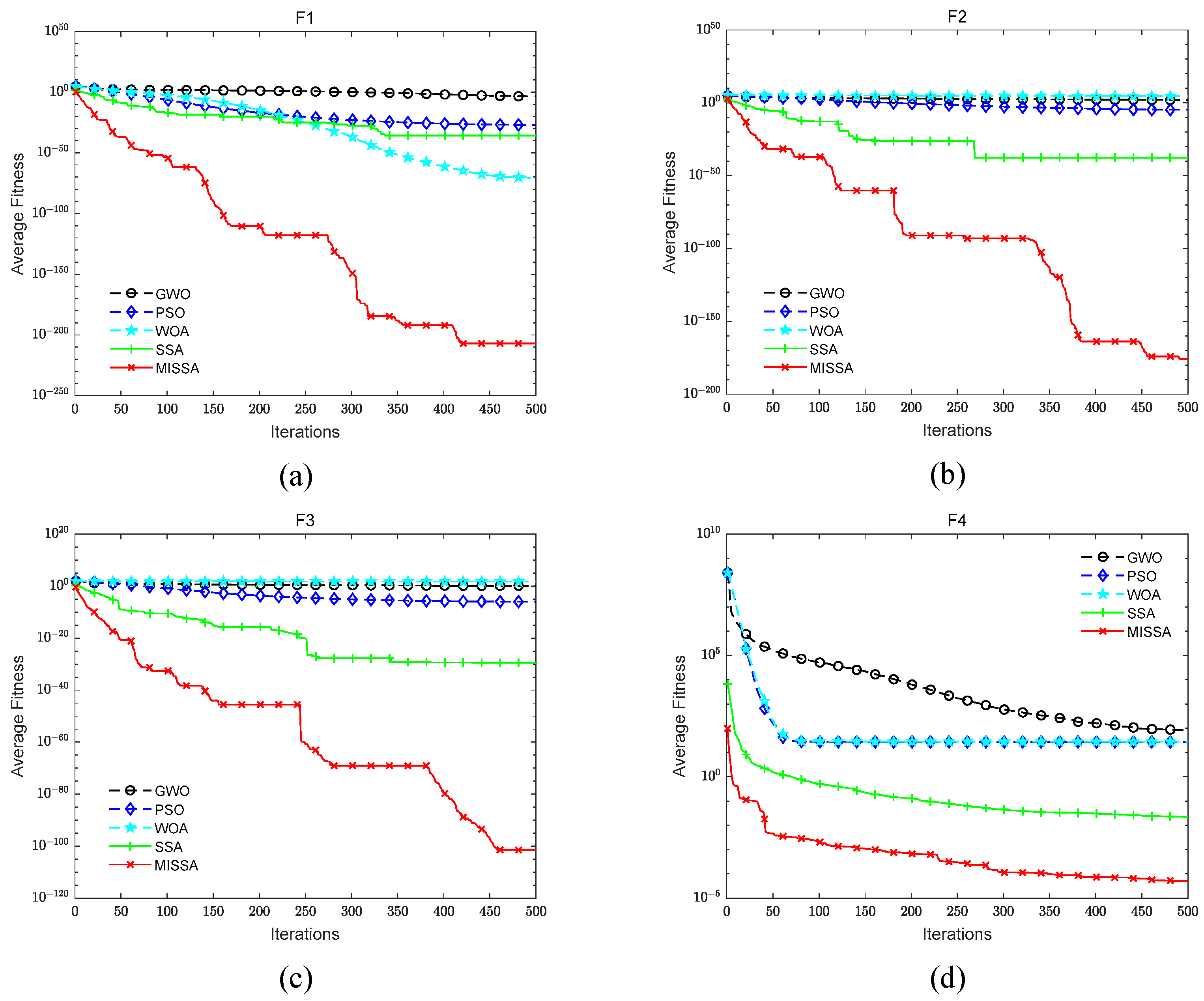
From Table 2, we know that in the solution of unimodal functions F1, F2 and F3, MISSA is the only one that can obtain the optimal solution, and the standard deviation of the F1 and F2 functions is also 0. When solving the function F1, only MISSA and SSA reach the optimal solution. Regarding the solution of unimodal functions F4 and F5, the average value and standard deviation of MISSA are obviously improved compared with other algorithms. MISSA is the best among the five algorithms for solving unimodal functions. In the last five multimodal functions, for the solution of F6 and F7, the accuracy and stability of MISSA and SSA are the same as the results. Still, in the resolution of F8, F9, and F10, the three indicators of MISSA are the best among the comparison algorithms.
To directly see the changes in the convergent speed and accuracy of various algorithms, the average fitness convergence of the five algorithms when solving ten benchmark functions is plotted. Figure 7 distinctly displays that when the optimization test is performed for ten benchmark functions, MISSA can achieve the desired effect relatively quickly and perform well.

5.2. Validation of MISSA-BP Surrogate Model

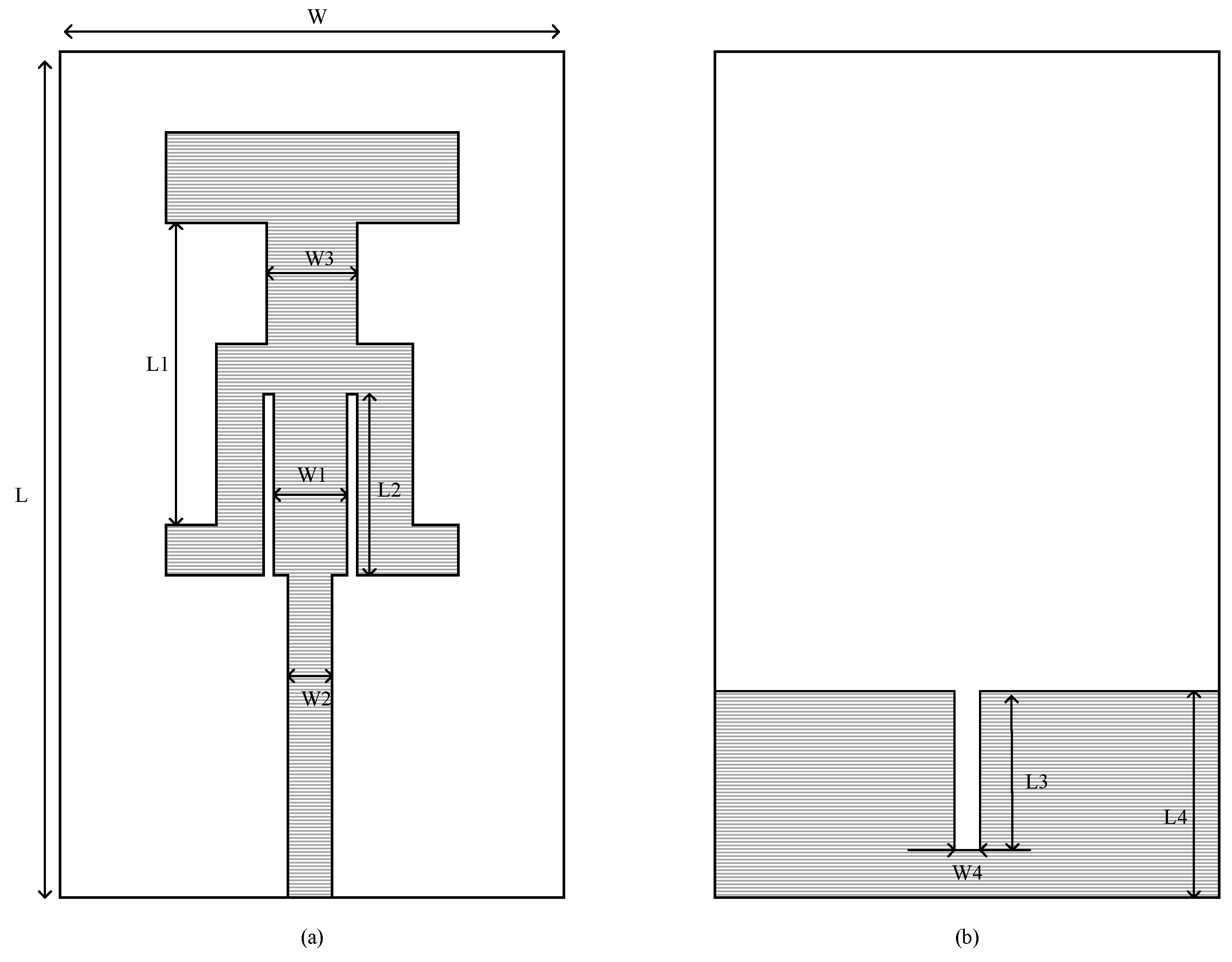
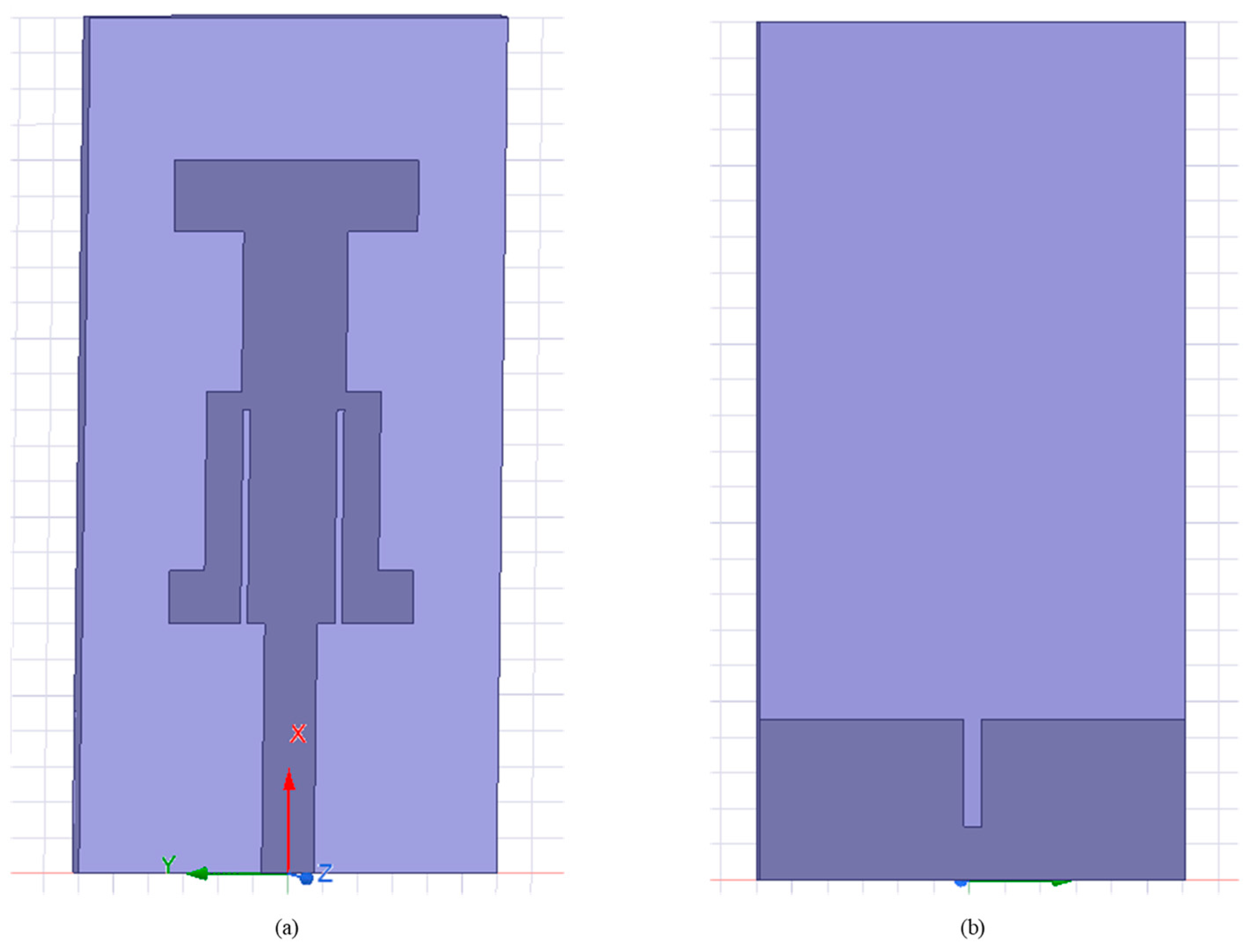
The structure of the tri-band antenna used in this paper is shown in Figure 8 [37]. Figure 9 shows the 3D view of the antenna in the high-frequency structure simulator (HFSS). Since the frequency band of this antenna is within 10 GHz, an FR-4 substrate is used. The dielectric constant of the substrate is 4.4, and the thickness is 1.6 mm. The FR-4 substrate has the characteristics of low cost and high flexibility, which is convenient for making the antenna into a real object later. Table 3 shows the length range of the tri-band antenna sizes.
Within the range given in Table 1, using LHS to obtain 100 groups of data. Then the data is simulated by using HFSS 2021 R1, the reflection coefficient is obtained, and 20 sampling frequency points are uniformly selected as a result of set R. 90 of the 100 sets of corresponding data are employed to train the network that we need. The remaining ten sets can be verified for the training effect. The number of input layer nodes of the BP neural network is the same as the antenna structure parameters in Table 1 (i.e., 10). The output layer nodes correspond to the selected 20 sampling frequency points (i.e., 20). To get the desired outcome, the number of hidden layer nodes is determined [15,25] for five tests, and it is found that selecting 17 nodes is the best. Therefore, the structure adopted by the neural network is 10-17-20, then using MISSA to deal with flaws of networks. According to the parameter settings of the literature and many tests, we determine some parameters of MISSA. The upper limit of the number of iterations is 100, the scale of the initial population is 30, the proportion of the finders is 0.2, the optimization result is substituted into the network structure, and the surrogate model based on MISSA-BP is obtained.
To prove relevant indicators of the surrogate model based on MISSA-BP, SVR [5], Kriging [8], PSO-BP, GWO-BP, WOA-BP, SSA-BP, and MISSA-BP surrogate models are constructed for performance comparison. The number of iterations is 200, and the other parameter settings are consistent with Section 5.1. The indicators of evaluation are mean square error (MSE) and mean absolute percentage error (MAPE).
M S E = 1 20 n = 1 20 R ( n ) R ¯ ( n ) 2
M A P E = n = 1 20 R ( n ) R ¯ ( n ) R ( n ) 20 × 100 %
where R ( n ) is the actual data of the electromagnetic software and R ¯ ( n ) is the simulation data obtained from the MISSA-BP model.
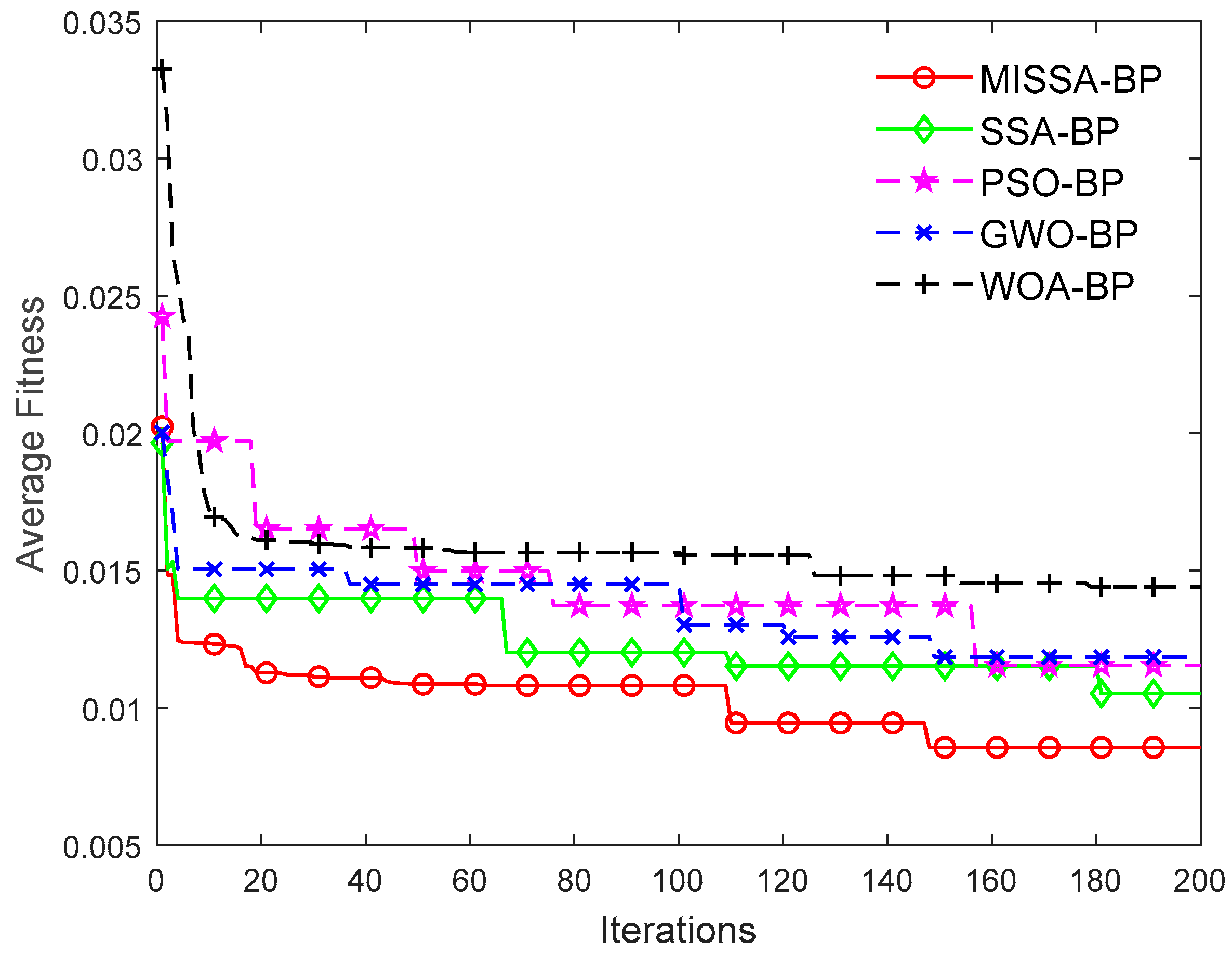
Each optimized surrogate model performs ten independent predictions on the test set, and Table 4 shows the average accuracy of prediction and time-consuming. The average training fitness iteration curves of PSO-BP, GWO-BP, WOA-BP, SSA-BP, and MISSA-BP surrogate models are shown in Figure 10.
From the data in Table 4, we can see that both MES and MAPE of the MISSA-BP surrogate model are obviously smaller than the other models, the accuracy is higher, and the time is shorter. Figure 10 shows that the MISSA-BP has the best fitness compared with other models in the same iteration times, and with the increase of iteration times, the performance of MISSA-BP becomes better and better. Therefore, the MISSA-BP model can substitute for the high-fidelity electromagnetic software and simultaneously design the antenna with the MOPSO algorithm.

5.3. Design of Multi-Objective Antenna

Using the MISSA-BP model constructed in part 5.2 united with MOPSO, the antenna is designed with multiple objectives. The design optimization objective of the antenna: (1) Keep the antenna as small as possible, i.e., F 1 = W × L . (2) Make the center frequency point of the antenna in the following range, 1.97–2.29 Ghz, 4.88–5.46 Ghz, and 7.18–7.54 Ghz works in S and C bands and can be applied to WLAN wireless network and high-frequency communication. The equations are as follows:
F 2 = n = 1 20 f ( x n ) 20
where   f ( x n ) = S 11 ( x n ) S 11 ( x n ) < 10   10 S 11 ( x n ) > 10
where x n is the nth sampling frequency point; S 11 ( x n ) is the reflection coefficient S 11 of the corresponding frequency point.
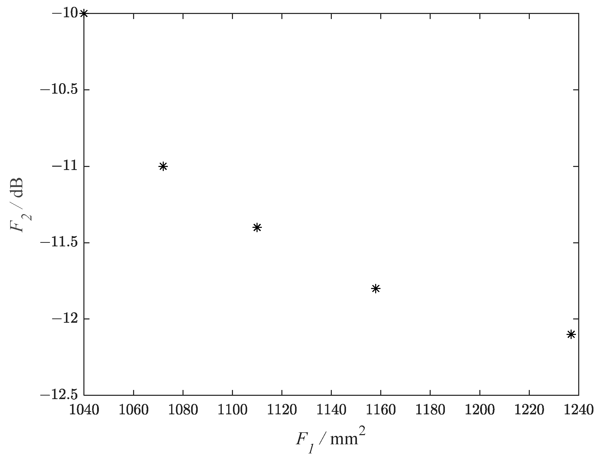
After multiple tests, the MOPSO parameters are set as below: particle swarm scale is 200, the dimension of the particle is 10, the upper limit of velocity is 1, the number of iterations is 300, and the weight parameter is reduced regular from 1 to 0.5, and the learning factor is 2.05. The MISSA-BP surrogate model and MOPSO start to iterate together to optimize objectives F1 and F2. The range of optimized antenna size parameters is given in Table 3. When MOPSO reaches the set number of iterations, the procedure ends, and the obtained Pareto Front is shown in Figure 11. In Figure 11, each point represents an antenna model. The antenna sizes can be obtained from the output data, which are within the specified range. The procedure is run repeatedly five times, each time selecting one from the obtained set of solutions. Table 5 shows the detailed sizes of the five antennas. It can be seen from Table 5 that all ten dimensions are within the range specified in Table 3 and meet the design requirements.
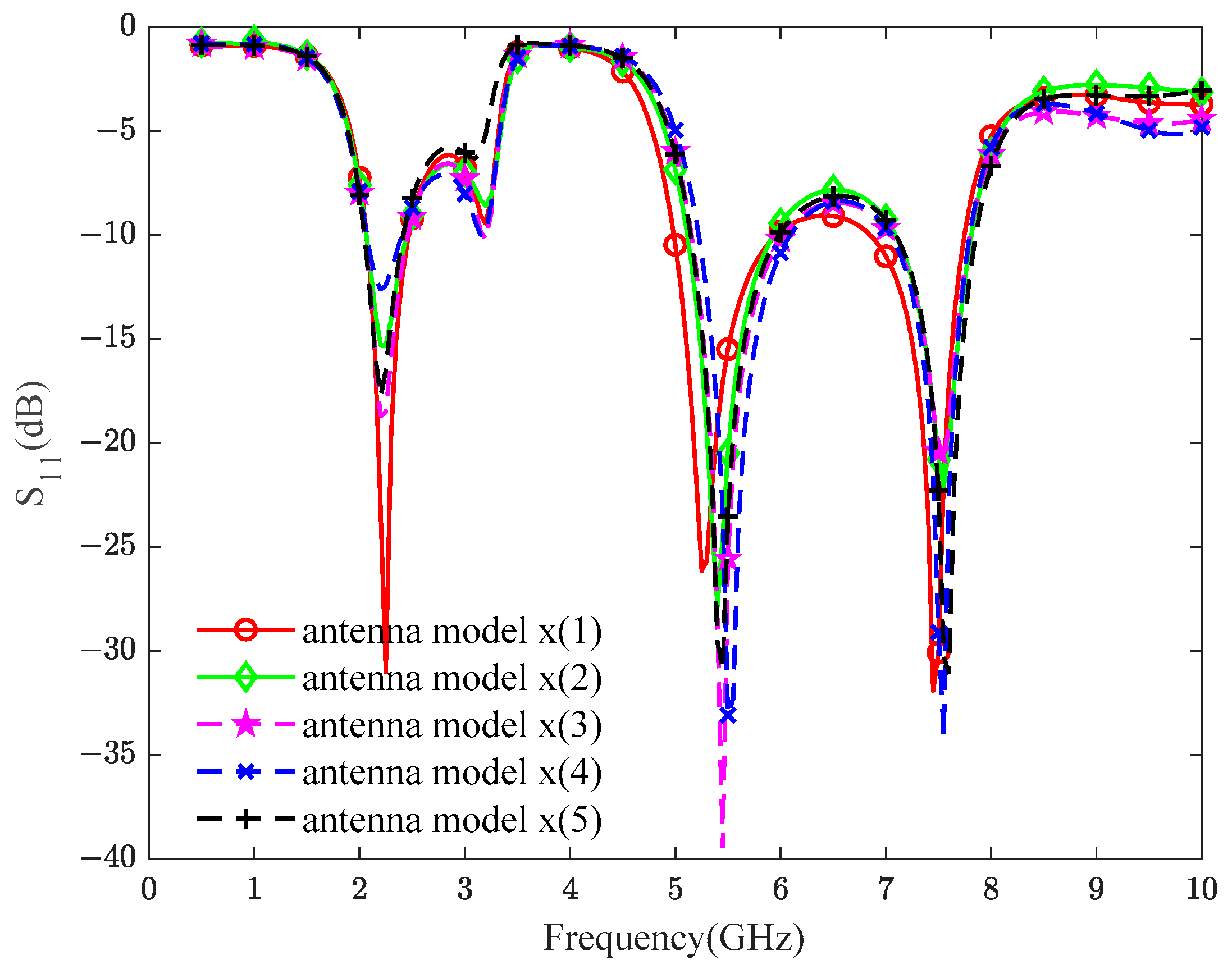
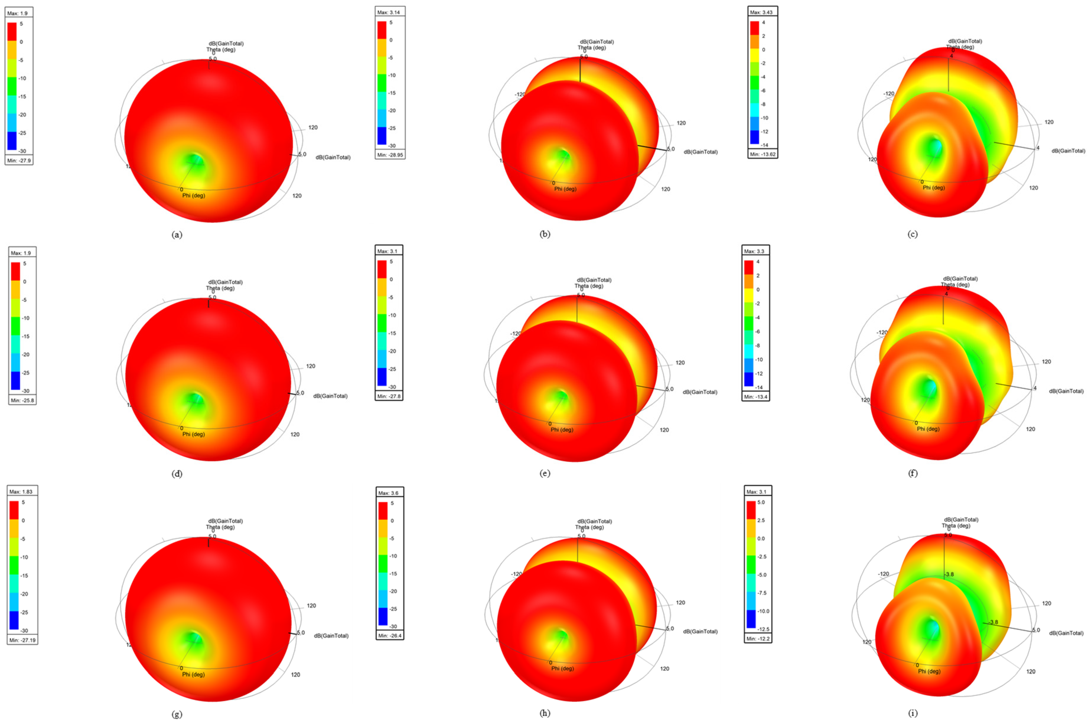
The reflection coefficient curves of the five groups of antennas simulated in HFSS software look like Figure 12. Furthermore, five groups of antenna models are simulated with the HFSS software for the 3D polar plot, and the results are shown in Figure 13. The 3D polar plot of the antenna is an important graph to measure the performance of the antenna, from which we can observe the parameters of the antenna, such as radiation direction, gain, etc. Figure 12 shows that the designed antennas meet objective F2, and the reflection coefficients are all less than −10 dB in the corresponding frequency band, which can work perfectly.
The planar tri-band antenna can meet the antenna design requirements in three frequency bands, less than −10 dB, which are suitable for WLAN wireless networks and high-frequency communication. It can be seen from Figure 13 that in the two-center frequencies of 2.17 GHz and 5.28 GHz, the 3D polar plots of antennas are relatively regular, indicating that the radiation direction is relatively uniform, and the gain is higher than 1.8 dB, which meets the design requirements. When the center frequency reaches 7.45 GHz, although the gain of the antenna is enhanced, the directivity becomes worse, resulting in the 3D directional map of the antenna becoming irregular. In general, the reflection coefficient and gain of the designed antenna can meet the requirements of the three-center frequency of 2.17 GHz, 5.28 GHz, and 7.45 GHz.
The time comparison between using HFSS electromagnetic simulation software and the method used in this paper to optimize the antenna structure is shown in Table 6. The running time of HFSS electromagnetic simulation software is about 47.70 s per simulation. The optimization of the antenna in this paper by HFSS requires about 1900 simulations, which takes 25.18 h in total. Using the method proposed in the paper to design the antenna, it takes one hundred simulations to build the model, and the total time is 1.55 h, which is only 6.14% of the HFSS method.
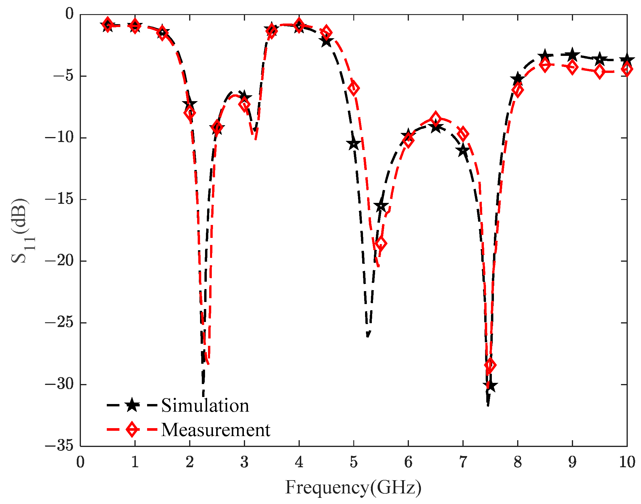
Finally, we have fabricated the antenna model x (1) in Table 5 and measured the reflection coefficient of the antenna. The real antenna is shown in Figure 14, and the measured results of the reflection coefficient are shown in Figure 15. It is easy to see from Figure 15 that the measured and simulated results of the antenna are very similar. The reflection coefficient is less than −10 dB in the three frequency bands, and the measured results conform to the expected objective. This further illustrates the effectiveness and practicality of the method proposed in this paper. From all the results above, it is demonstrated that the proposed method has high prediction accuracy, dramatically improves the time-consuming aspect, and can quickly design the antenna to meet the requirements.

6. Conclusions

This paper presents a design method for the multi-objective antenna, which can be used to design the antenna quickly. This method is implemented using an improved SSA to optimize the surrogate model. First, the sparrow search algorithm is improved by using three strategies, namely the chaotic map, inertia weight, and t-distribution, to enhance its searchability and optimization performance. Secondly, the proposed new algorithm is applied to the original neural network, and the surrogate model based on MISSA-BP is constructed. Finally, the surrogate model is united with the MOPSO algorithm to resolve the difficulties in multi-objective antenna design. The relevant results state that MISSA performs better, and this MISSA-BP model can accurately predict the performance of the antenna. The accuracy is significantly improved and less time-consuming. This method has good practical value and significance for the design of the multi-objective antenna.

Author Contributions

Conceptualization, Z.W. and J.Q.; methodology, Z.W. and J.Q.; software, Z.H. and J.H.; validation, Z.H., J.H. and D.T.; formal analysis, Z.W. and J.Q.; data curation, Z.W., Z.H., J.Q. and D.T.; writing—original draft preparation, Z.W., Z.H. and J.H.; writing—review and editing, J.Q. and D.T.; funding acquisition, J.Q. and D.T. All authors have read and agreed to the published version of the manuscript.

Funding

This work is supported by Science and Technologies Plan Projects of Guangzhou City under Grant 202002030407; in part by the Guangdong Basic and Applied Basic Research Foundation under Grant 2021A1515012566; in part by the Science and Technologies of Guangzhou university under Grant PTZC2022015.

Institutional Review Board Statement

Not applicable.

Informed Consent Statement

Not applicable.

Data Availability Statement

The dataset generated and analyzed during the current study is available from the corresponding author on reasonable request.

Conflicts of Interest

The authors declare no conflict of interest.

References

  1. Dong, J.; Li, Y.; Wang, M. Fast Multi-Objective Antenna Optimization Based on RBF Neural Network Surrogate Model Optimized by Improved PSO Algorithm. Appl. Sci. 2019, 9, 2589. [Google Scholar] [CrossRef] [Green Version]
  2. Koziel, S.; Adrian, B. Rapid multi-objective antenna design using point-by-point Pareto set identification and local surrogate models. IEEE Trans. Antennas Propag. 2016, 64, 2551–2556. [Google Scholar] [CrossRef]
  3. Bekasiewicz, A.; Koziel, S.; Plotka, P.; Zwolski, K. EM-Driven Multi-Objective Optimization of a Generic Monopole Antenna by Means of a Nested Trust-Region Algorithm. Appl. Sci. 2021, 11, 3958. [Google Scholar] [CrossRef]
  4. Dong, J.; Qin, W. Fast Multi-Objective Optimization of Multi-Parameter Antenna Structures Based on Improved BPNN Surrogate Model. IEEE Access 2019, 7, 77692–77701. [Google Scholar] [CrossRef]
  5. Prado, D.R.; López-Fernández, J.A.; Arrebola, M. Wideband shaped-beam reflect array design using support vector regression analysis. IEEE Antennas Wirel. Propag. Lett. 2019, 18, 2287–2291. [Google Scholar] [CrossRef] [Green Version]
  6. Gao, J.; Tian, Y.; Chen, X. Antenna optimization based on co-training algorithm of Gaussian process and support vector machine. IEEE Access 2020, 8, 211380–211390. [Google Scholar] [CrossRef]
  7. Koziel, S.; Bekasiewicz, A. Fast multi-objective surrogate-assisted design of multi-parameter antenna structures through rotational design space reduction. IET Microw. Antennas Propag. 2016, 10, 624–630. [Google Scholar] [CrossRef]
  8. Xia, B.; Ren, Z.; Koh, C.S. Utilizing Kriging Surrogate Models for Multi-Objective Robust Optimization of Electromagnetic Devices. IEEE Trans. Magn. 2014, 50, 693–696. [Google Scholar] [CrossRef]
  9. Koziel, S.; Ogurtsoy, S. Multi-objective design of antennas using variable-fidelity simulations and surrogate models. IEEE Trans. Antennas Propag. 2013, 61, 5931–5939. [Google Scholar] [CrossRef]
  10. Tak, J.; Kantemur, A.; Sharmma, Y. A 3-D-printed W-band slotted waveguide array antenna optimized using machine learning. IEEE Antennas Wirel. Propag. Lett. 2018, 17, 2008–2012. [Google Scholar] [CrossRef]
  11. Patnaik, A.; Sinha, S.N. Design of Custom-Made Fractal Multi-Band Antennas Using ANN-PSO Antenna Designer’s Notebook. IEEE Antennas Propag. Mag. 2011, 53, 94–101. [Google Scholar] [CrossRef]
  12. Mishra, S.; Yadav, R.N.; Singh, R.P. Directivity estimations for short dipole antenna arrays using radial basis function neural networks. IEEE Antennas Wirel. Propag. Lett. 2015, 14, 1219–1222. [Google Scholar] [CrossRef]
  13. Reddy, B.; Vakula, D. Single aperture multiple beams of array antenna using Radial Basis Function Neural Network. In Proceedings of the 2015 IEEE MTT-S International Microwave and RF Conference (IMaRC), Hyderabad, India, 10–12 December 2015; pp. 388–391. [Google Scholar]
  14. Gao, Y.; Ji, W.; Zhao, X. SOC Estimation of E-Cell Combining BP Neural Network and EKF Algorithm. Processes 2022, 10, 1721. [Google Scholar] [CrossRef]
  15. Hu, W.; Jin, S.; Zhou, J.; Yang, J.; Luo, Y.; Shi, Y.; Sun, C.; Jiang, P. Prediction of the Equivalent Steering Angle of a Front-Wheel, High-Clearance Paddy Field Management Machine. Appl. Sci. 2022, 12, 7802. [Google Scholar] [CrossRef]
  16. Dong, J.; Qin, W.; Mo, J. Low-cost multi-objective optimization of multi-parameter antenna structures based on the l1 optimization BPNN surrogate model. Electronics 2019, 8, 839. [Google Scholar] [CrossRef] [Green Version]
  17. Wang, L.; Liang, Z.C.; Pu, Y. Method for Loran-C Additional Secondary Factor Correction Based on Neural Network and Transfer Learning. IEEE Antennas Wirel. Propag. Lett. 2021, 21, 332–336. [Google Scholar] [CrossRef]
  18. Zhu, W.; Guo, L.; Jia, Z.; Tian, D.; Xiong, Y. A Surrogate-Model-Based Approach for the Optimization of the Thermal Design Parameters of Space Telescopes. Appl. Sci. 2022, 12, 1633. [Google Scholar] [CrossRef]
  19. Bai, Y.; Luo, M.; Pang, F. An Algorithm for Solving Robot Inverse Kinematics Based on FOA Optimized BP Neural Network. Appl. Sci. 2021, 11, 7129. [Google Scholar] [CrossRef]
  20. Zhang, R.; Xu, Z.B.; Huang, G.B.; Wang, D.H. Global convergent of online BP training with dynamic learning rate. IEEE Trans. Neural Netw. Learn. Syst. 2012, 23, 330–341. [Google Scholar] [CrossRef]
  21. Xu, Z.B.; Zhang, R.; Jing, W.F. When Does Online BP Training Converge? IEEE Trans. Neural Netw. 2009, 20, 1529–1539. [Google Scholar] [CrossRef]
  22. Xue, J.; Shen, B. A novel swarm intelligence optimization approach: Sparrow search algorithm. Syst. Sci. Control. Eng. 2020, 8, 22–34. [Google Scholar] [CrossRef]
  23. Yan, P.; Shang, S.; Zhang, C. Research on the Processing of Coal Mine Water Source Data by Optimizing BP Neural Network Algorithm with Sparrow Search Algorithm. IEEE Access 2021, 9, 108718–108730. [Google Scholar] [CrossRef]
  24. Li, N.; Wang, W. Prediction of Mechanical Properties of Thermally Modified Wood Based on TSSA-BP Model. Forests 2022, 13, 160. [Google Scholar] [CrossRef]
  25. Nguyen, T.-T.; Ngo, T.-G.; Dao, T.-K.; Nguyen, T.-T.-T. Microgrid Operations Planning Based on Improving the Flying Sparrow Search Algorithm. Symmetry 2022, 14, 168. [Google Scholar] [CrossRef]
  26. Wu, C.; Fu, X.; Dong, Z. A Novel Sparrow Search Algorithm for the Traveling Salesman Problem. IEEE Access 2021, 9, 153456–153471. [Google Scholar] [CrossRef]
  27. Yan, S.; Yang, P.; Zhu, D. Improved sparrow search algorithm based on iterative local search. Comput. Intell. Neurosci. 2021, 2021, 6860503. [Google Scholar] [CrossRef] [PubMed]
  28. Jianhua, L.; Zhiheng, W. A hybrid sparrow search algorithm based on constructing similarity. IEEE Access 2021, 9, 117581–117595. [Google Scholar] [CrossRef]
  29. Kennedy, J.; Eberhart, R. Particle swarm optimization. In Proceedings of the ICNN’95-International Conference on Neural Networks, Perth, WA, Australia, 27 November–1 December 1995; Volume 4, pp. 1942–1948. [Google Scholar] [CrossRef]
  30. Mirjalili, S.; Mirjalili, S.M.; Lewis, A. Grey wolf optimizer. Adv. Eng. Softw. 2014, 69, 46–61. [Google Scholar] [CrossRef] [Green Version]
  31. Mirjalili, S.; Lewis, A. The Whale Optimization Algorithm. Adv. Eng. Softw. 2016, 95, 51–67. [Google Scholar] [CrossRef]
  32. Ali, M.H.; Salawudeen, A.T.; Kamel, S.; Salau, H.B.; Habil, M.; Shouran, M. Single- and Multi-Objective Modified Aquila Optimizer for Optimal Multiple Renewable Energy Resources in Distribution Network. Mathematics 2022, 10, 2129. [Google Scholar] [CrossRef]
  33. Liu, W.; Zhang, J.; Wei, W.; Qin, T.; Fan, Y.; Long, F.; Yang, J. A Hybrid Bald Eagle Search Algorithm for Time Difference of Arrival Localization. Appl. Sci. 2022, 12, 5221. [Google Scholar] [CrossRef]
  34. Li, W.; He, Z.; Zheng, J. Improved flower pollination algorithm and its application in user identification across social networks. IEEE Access 2019, 7, 44359–44371. [Google Scholar] [CrossRef]
  35. Qu, Y.; Yang, T.; Li, T.; Zhan, Y.; Fu, S. Path Tracking of Underground Mining Boom Roadheader Combining BP Neural Network and State Estimation. Appl. Sci. 2022, 12, 5165. [Google Scholar] [CrossRef]
  36. Xue, B.; Zhang, M.; Browne, W.N. Particle swarm optimization for feature selection in classification: A multi-objective approach. IEEE Trans. Cybern. 2012, 43, 1656–1671. [Google Scholar] [CrossRef] [PubMed]
  37. Misra, P.; Tripathy, A. Triple Band Planar Antenna for Wireless Communication. Int. J. Comput. Appl. 2012, 48, 28–30. [Google Scholar] [CrossRef]
Figure 1. Distribution histogram of three chaotic mappings: (a) distribution histogram of Logistic mapping; (b) distribution histogram of Tent mapping; (c) distribution histogram of Bernoulli mapping.
Applsci 12 12543 g001
Figure 2. Changes in the location of the finder.
Applsci 12 12543 g002
Figure 3. Iterative change of adaptive weight.
Applsci 12 12543 g003
Figure 4. Flow chart of MISSA.
Applsci 12 12543 g004
Figure 5. Structure of BP neural network model.
Applsci 12 12543 g005
Figure 6. Flow chart of antenna design based on MISSA-BP.
Applsci 12 12543 g006
Figure 7. Convergent curve of five algorithms on ten benchmarks functions: (a) function F1; (b) function F2; (c) function F3; (d) function F4; (e) function F5; (f) function F6; (g) function F7; (h) function F8; (i) function F9; (j) function F10.
Applsci 12 12543 g007aApplsci 12 12543 g007b
Figure 8. Structure diagram of planar tri-band antenna: (a) front structure of the antenna; (b) reverse structure of the antenna.
Applsci 12 12543 g008
Figure 9. 3D view of the planar tri-band antenna in HFSSS: (a) front view of the antenna; (b) reverse view of the antenna.
Applsci 12 12543 g009
Figure 10. Iteration curve of the average fitness of the surrogate model.
Applsci 12 12543 g010
Figure 11. Pareto Front of the planar tri-band antenna.
Applsci 12 12543 g011
Figure 12. Simulated results of the reflection coefficient of antenna models.
Applsci 12 12543 g012
Figure 13. Simulated results from the obtained structure of the tri-band antenna of HFSS: (a) 3D polar plot of antenna model x (1) at 2.17 GHz; (b) 3D polar plot of antenna model x (1) at 5.28 GHz; (c) 3D polar plot of antenna model x (1) at 7.45 GHz; (d) 3D polar plot of antenna model x (2) at 2.17 GHz; (e) 3D polar plot of antenna model x (2) at 5.28 GHz; (f) 3D polar plot of antenna model x (2) at 7.45 GHz; (g) 3D polar plot of antenna model x (3) at 2.17 GHz; (h) 3D polar plot of antenna model x (3) at 5.28 GHz; (i) 3D polar plot of antenna model x (3) at 7.45 GHz; (j) 3D polar plot of antenna model x (4) at 2.17 GHz; (k) 3D polar plot of antenna model x (4) at 5.28 GHz; (l) 3D polar plot of antenna model x (4) at 7.45 GHz; (m) 3D polar plot of antenna model x (5) at 2.17 GHz; (n) 3D polar plot of antenna model x (5) at 5.28 GHz; (o) 3D polar plot of antenna model x (5) at 7.45 GHz.
Applsci 12 12543 g013aApplsci 12 12543 g013b
Figure 14. The real antenna: (a) front structure of the antenna; (b) reverse structure of the antenna.
Applsci 12 12543 g014
Figure 15. Simulated and measured reflection coefficients of the antenna.
Applsci 12 12543 g015
Table 1. Benchmark function.
TypeExpressionDimensionRangeOptimal Value
F 1 ( x ) = i = 1 n x i 2 30[−100, 100]0
Unimodal function F 2 ( x ) = i = 1 n j = 1 n x j 2 30[−100, 100]0
F 3 ( x ) = max i = 1 n { x i , 1 i n } 30[−100, 100]0
F 4 ( x ) = i = 1 n [ 100 ( x i + 1 x i 2 ) 2 + ( x i 1 ) 2 ] 30[−30, 30]0
F 5 ( x ) = i = 1 n x i + 0.5 2 30[−100, 100]0
Multimodal function


Multimodal function
F 6 ( x ) = 20 exp 0.2 1 n i = 1 n x i 2 exp 1 n i = 1 n cos ( 2 π x i ) ) + 20 + e 30[−32, 32]0
F 7 ( x ) = 1 4000 i = 1 n x i 2 i = 1 n cos x i i + 1 30[−600, 600]0
F 8 ( x ) = 1 500 + j = 1 25 1 j + i = 1 2 ( x i a i j ) 6 1 2[−65, 65]1
F 9 ( x ) = i = 1 11 a i x 1 ( b i 2 + b i x 2 ) b i 2 + b i x 3 + x 4 2 6[−5, 5]0.0003
F 10 ( x ) = i = 1 5 ( X a i ) ( X a i ) T + c i 1 4[0, 10]−10.153
Table 2. Benchmark function test results.
FunctionStatistical ValuePSOGWOWOASSACASSA
F1Optimal value2.121 × 10−63.455 × 10−293.409 × 10−8400
Average value3.596 × 10−41.118 × 10−271.488 × 10−711.777 × 10−368.481 × 10−208
Standard deviation0.001 × 10−11.843 × 10−278.126 × 10−719.732 × 10−360
F2Optimal value2.120 × 1011.148 × 10−081.715 × 10−42.485 × 10−1500
Average value8.659 × 1011.617 × 10−054.397 × 10−42.544 × 10−381.221 × 10−176
Standard deviation3.380 × 1015.478 × 10−051.561 × 10−41.393 × 10−370
F3Optimal value8.659 × 10−11.308 × 10−71.343 × 10−21.475 × 10−1250
Average value1.167 × 1009.467 × 10−75.788 × 1012.822 × 10−303.130 × 10−102
Standard deviation0.255 × 1009.013 × 10−72.941 × 1011.546 × 10−291.715 × 10−101
F4Optimal value1.979 × 1012.612 × 1012.705 × 1019.946 × 10−56.366 × 10⁻⁹
Average value8.433 × 1012.714 × 1012.774 × 1012.205 × 10−24.824 × 10⁻⁵
Standard deviation6.299 × 1015.031 × 1013.579 × 1011.573 × 10−27.446 × 10⁻⁵
F5Optimal value1.439 × 10−58.346 × 10−51.032 × 10−12.512 × 10−56.265 × 10−12
Average value9.862 × 10−57.996 × 10−13.877 × 10−11.128 × 10−43.552 × 10−7
Standard deviation9.323 × 10−53.995 × 10−12.774 × 10−19.484 × 10−55.638 × 10−7
F6Optimal value2.047 × 10−36.484 × 10−148.882 × 10−168.882 × 10−168.882 × 10⁻¹⁶
Average value1.954 × 10−19.780 × 10−144.204 × 10−158.882 × 10−168.882 × 10⁻¹⁶
Standard deviation4.740 × 10−11.706 × 10−142.072 × 10−1500
F7Optimal value1.225 × 10−60000
Average value7.894 × 10−34.795 × 10−35.600 × 10−300
Standard deviation9.217 × 10−37.407 × 10−33.067 × 10−200
F8Optimal value9.980 × 10−19.980 × 10−19.980 × 10−19.980 × 10−19.980 × 10−1
Average value3.619 × 1004.647 × 1002.412 × 1009.047 × 1009.980 × 10−1
Standard deviation3.290 × 1004.597 × 1002.196 × 1004.701 × 1003.172 × 10−8
F9Optimal value6.058 × 10−43.075 × 10−43.085 × 10−43.075 × 10−43.074 × 10−4
Average value9.094 × 10−43.758 × 10−35.781 × 10−43.737 × 10−43.129 × 10−4
Standard deviation1.217 × 10−47.557 × 10−33.153 × 10−41.686 × 10−45.753 × 10−6
F10Optimal value−1.015 × 101−1.015 × 101−1.015 × 101−1.015 × 101−1.015 × 101
Average value−7.699 × 100−9.315 × 100−8.271 × 100−1.015 × 101−1.015 × 101
Standard deviation2.927 × 1002.216 × 1002.722 × 1006.009 × 10−43.860 × 10⁻⁶
Table 3. Length range of the tri-band antenna sizes (unit: mm).
ParameterWW1W2W3W4
Range[22, 26][4, 6][2.5, 3.5][1.5, 2.5][0.5, 1.5]
ParameterLL1L2L3L4
Range[48, 50][18, 20][11, 13][6, 8][8, 10]
Table 4. Prediction accuracy of each optimized agent model.
Surrogate ModelMSEMAPE/ (%)Time-Consuming (s)
SVR [5]3.8619.6915.56
Kriging [8]3.7816.7614.33
BP3.7015.6810.12
PSO-BP2.7411.359.92
GWO-BP3.0511.879.61
WOA-BP3.4212.029.57
SSA-BP2.0510.159.32
MISSA-BP0.877.147.16
Table 5. Optimal size parameters of the tri-band antenna (unit: mm).
WW1W2W3W4LL1L2L3L4
antenna model x (1)23.265.963.321.810.9948.6319.8711.056.499.88
antenna model x (2)22.555.643.091.641.4948.2818.9011.257.099.33
antenna model x (3)24.435.553.332.111.3149.2119.1211.066.119.94
antenna model x (4)23.395.032.932.101.1949.2019.1111.096.369.96
antenna model x (5)23.465.073.371.860.7548.7318.7311.637.049.97
Table 6. Time comparison of different antenna optimization methods (unit: s).
Optimization MethodSurrogate ModelMulti-Objective OptimizationCPU Time
TotalRelative (%)
HFSS--90,630100
Proposed method477079855686.14
Publisher’s Note: MDPI stays neutral with regard to jurisdictional claims in published maps and institutional affiliations.