Short Term Prediction Model of Environmental Parameters in Typical Solar Greenhouse Based on Deep Learning Neural Network

Abstract

The type of single-slope solar greenhouse is mainly used for vegetable production in China. The coupling of heat storage and release courses and the dynamic change in the outdoor weather parameters momentarily affect the indoor environment. Due to the high cost of small weather stations, the environmental parameters monitored by the nearest meteorological stations are usually used as outdoor environmental parameters in China. In order to accurately predict the solar greenhouse and crop water demand, this paper proposes three deep learning models, including neural network regression (DNNR), long short-term memory (LSTM), and convolutional neural network-long- short-term memory (CNN-LSTM), and the hyperparameters of three models were determined by orthogonal experimental design (OD). The temperature and relative humidity monitored by the indoor sensors and outdoor weather station were taken as the inputs of models, the temperature and relative humidity 3, 6, 12 and 24 h in advance were taken as the output, 16 combinations of input and output data of two typical solar greenhouses were trained separately by three deep learning models, those models were trained 144, 144 and 288 times, respectively. The best model of three type models at four prediction time points were selected, respectively. For the forecast time point of 12 h in advance, the errors of the best LSTM and CNN-LSTM models in two greenhouses were all smaller than the DNNR models. For the three other time points, the results show that the DNNR models have excellent prediction accuracy among the three models. The maximum and minimum temperature, relative humidity, and ET_o were also accurately predicted using the corresponding optimized models. In sum, this study provided an optimized deep learning prediction model for environmental parameters of greenhouse and provides technical support for irrigation decision-making and water allocation.

1. Introduction

An agricultural greenhouse can provide relatively suitable growing conditions for crops in all seasons. An agricultural greenhouse is the main way of facilitating precise agriculture and efficient agriculture production [1]. There are 1.96 million hectares of single-slope solar greenhouses in northern China, which are the main type of greenhouse for vegetable production. The walls of most solar greenhouses consist of rammed soil, and the total area of most solar greenhouses range from 300 m² to 1200 m² [2,3].

For many greenhouse environmental parameters, temperature and relative humidity in greenhouses are the main factors affecting the healthy growth and yield of crops, and are the key to achieving the relative stability of its internal environment [4]. The core of greenhouse environmental system modeling is the relationship between environment parameters and crop production. Those greenhouse environmental parameters have been documented to be sensitive to greenhouse structure and outdoor weather variation, which were considered dynamic and complex systems [5,6]. In recent years, a lot of studies have been conducted on greenhouse environmental modeling. Modeling methods for greenhouses can be divided into mechanism model, time series model and artificial intelligence model [1], those mechanism methods were dependent on physiological processes, and they represent crop growth, and yield as a function of several climate and physiological parameters [7]. A large number of environmental parameters need to be considered when building a mechanism model, and the unmeasurable environmental parameters were estimated or calculated. Because the other two models do not focus on the laws and principles of physics in the greenhouse, they are called Black-Box models. These two methods provide rapid and accurate results for greenhouse environmental prediction and regulation, for example, the temperature, humidity or reference evapotranspiration inside the greenhouse, and the planning of irrigation strategies [8].

A Kalman filter or extended Kalman filter is applicable to linear systems and has been introduced in the literature. It is not easy to derive the Jacobian matrix for the nonlinearization process, which often leads to major difficulties in implementation [9,10]. With the rapid development of computer technology and artificial intelligence technology, many excellent algorithms have been proposed to solve various complex problems involved in the greenhouse environment model, such as Kth-nearest neighbor (KNN), back-propagation (BP) neural networks, artificial neural network (ANN) [11], multi-layer perceptron (MLP), classification and regression tree (CART), support vector machines (SVM), wavelet neural network (WNN) and radial basis function (RBF) [12,13,14,15,16,17,18,19,20,21,22,23]. These algorithms are effective for the construction of temperature field, the solar radiation field, and the other nonlinear physical phenomena in greenhouse. However, those approaches still have some drawbacks, for example, poor applicability, overfitting, poor robustness and poor stability to actual strongly coupled and complex systems.

Deep learning (DL) can solve complex problems particularly well and quickly, due to the more complex models used, which also allow massive parallelization. The deep learning technology including recurrent neural networks (RNN), long short-term memory (LSTM), deep learning neural networks (DLNN) and convolutional neural networks (CNN) have been used to deal with the complex systems and prediction problems in the agricultural industry. Time series prediction based on LSTM models has been widely applied in various fields in recent years, including the prediction model of greenhouse environmental parameters. Jung et al. [8] developed a model to predict indoor temperature, relative humidity, and CO₂ concentration of a greenhouse using outdoor weather data and historical data, and the model was used to irrigation management of greenhouse tomatoes. Alhnaity et al. [24] developed a DL approach using LSTM for Ficus growth, tomato yield prediction in greenhouse environment, achieving high prediction accuracy. Codeluppi et al. [25] used LSTM, RNNs and ANNs for greenhouse air temperature forecasting. Liu et al. [26] proposed a model using LSTM to predict the indoor temperature, humidity, light, carbon dioxide concentration, soil temperature and soil humidity. Considering the most influential environmental parameters, including soil moisture, air temperature and humidity, carbon dioxide concentration and light intensity, Bhat et al. [27] developed a BO-DNN model for classification of the rose yield environment. In order to reduce time complexity, Lee et al. [28] developed a model using environmental information of adjacent areas.

Although there have been many studies on the environmental parameters of solar greenhouses, the models of these studies are difficult to apply to the actual solar greenhouse. Because the internal space of a solar greenhouse is small, the changes in its internal environmental parameters are gradual. Therefore, the cost of environmental parameter sensor inside the greenhouse is low, and the monitoring accuracy is higher. In contrast, the outdoor environmental parameters of solar greenhouses are usually monitored by small weather stations, the monitoring coverage of weather stations is relatively small, and the outdoor environment of the solar greenhouse is complex and changeable, and the accuracy of environmental parameters collected by small weather stations is relatively poor.

Although there have been many related studies on solar greenhouses, due to the lack of reliable data from small-scale meteorological stations and the output of numerical weather models on these time scales, it is very difficult to accurately predict the greenhouse environmental parameters in the short term (1~24 h). Indeed, the correctness of the reference evapotranspiration (ET_o) forecast also remains a challenging computational task. The solar greenhouse is a non-linear and dynamic system, in order to adjust the greenhouse environmental parameters accurately and timely, we need to predict the indoor environmental parameters in advance. Deep learning models are usually used to predict nonlinear and dynamic system, these models can also be applied to the prediction of greenhouse environmental parameters. In this study, three deep learning models (DNNR, LSTM, and CNN-LSTM) were constructed to simulate and predict the indoor environmental parameters of two typical greenhouses.

The architecture and hyperparameters are the main factors affecting the prediction accuracy of the deep learning models. It is essential to optimize the architecture and hyperparameters of those models. Grid search is one of the most commonly applied methods to optimize the hyperparameters. However, when the dimension of the hyperparameter is large, the time cost is very high. Some scholars have used an orthogonal design method to optimize the hyperparameters of the deep learning model. In the study, the orthogonal design was also used to optimize the important hyperparameters of three models. Therefore, considering the short-term change in outdoor parameters have great influence on the indoor environmental parameters, the models were trained and tested at four forecast time points, and at the same time, the minimum amount of necessary data was also determined. Finally, a comparison was made between ET_o computed with the predicted environmental parameters and the actual ET_o. In general, in order to predict short-term indoor environmental parameters and crop water consumption of solar greenhouse, this paper optimizes three deep learning prediction models through orthogonal experimental design to obtain the best prediction model.

Compared with the reported related studies, the main novelties of this study are highlighted below.

• Three general deep learning prediction models of environmental parameters for two typical solar greenhouses in dynamic conditions were presented, and the hyperparameters of the models were optimized using the orthogonal design method.
• Among the three types of models, the DNNR model has the best prediction performance. Providing multi-step ahead prediction of solar environment parameters for 3, 6, 12 and 24 h ahead.
• The accuracy of short-term predicted ET_o calculated with the predicted inner solar greenhouse environmental parameters was significantly improved.

2. Materials and Methods

This section summarizes the structure and geographical location of two typical solar greenhouses, the sensors for collecting the environmental data inside the greenhouse, the meteorological data sources of the adjacent stations of the greenhouse, and the irrigation water prediction model.

2.1. Experimental Greenhouses

In this study, the environmental parameters from two typical solar greenhouse are used to verify the deep learning model, one greenhouse is located in Yanling, on Xurong farm (Greenhouse A, 34.27° N, 108.11° E, 34 × 10 m, 340 m²), Xianyang, Shaanxi province, China, where data were collected from 1 May 2018 to 20 July 2018. The second greenhouse is located in Shouguang (Greenhouse B, 36.91° N, 118.86° E, 67 × 10 m, 670 m²), Weifang, Shandong province, China, where data were collected from 1 May 2020 to 20 June 2020. These two greenhouses are typical single slope solar greenhouses, with polyethylene film on the roof and a wall on the north side. The schematic diagram of two experimental solar greenhouses from the study is shown in Figure 1. The north wall of Greenhouse A is composed of two concrete walls and was filled with phase change cured soil, the north wall of Greenhouse B consists of compacted soil. The Yangling meteorological station (#57123, 34.28° N, 108.08° E) and the Shouguang meteorological station (#54832, 36.88° N, 118.74° E) are the closest national stations to Greenhouse A and Greenhouse B, respectively [29].

2.2. Data Collection and Overview

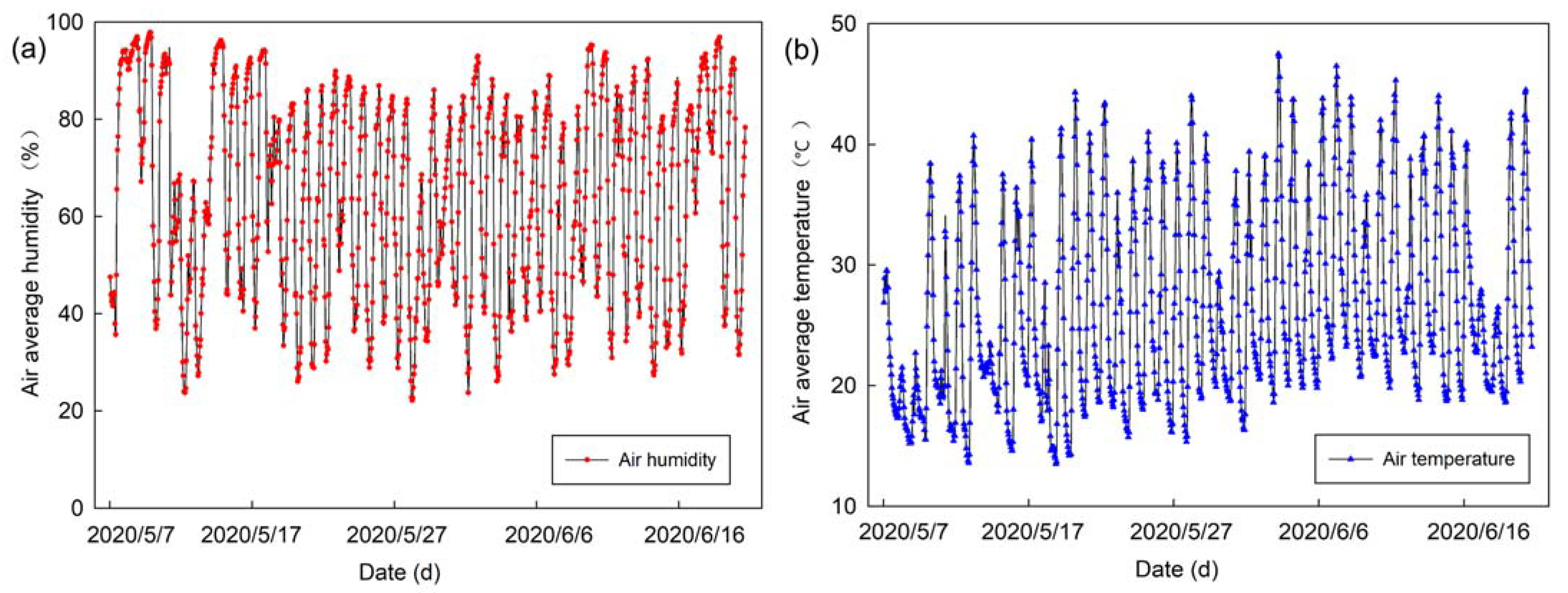
The inside environmental parameters (temperature, humidity, and radiation) were measured by the sensors in the center of the greenhouse. Temperature and humidity (RS-WS-N01-2, Shandong Jianda Renke Measurement and Control Technology Co., Ltd., Jinan, China) were installed 2 m above the ground, solar radiation was monitored with a radiation sensor (RS-GH, Shandong Jianda Renke Measurement and Control Technology Co., Ltd., Jinan, China), it was also installed 2 m above the ground. The three environmental datapoints were collected in one minute and uploaded to the cloud platform (T-Link, https://www.tlink.io/, accessed on 15 July 2020), and 1073 internal environmental parameters and weather environmental data sets were obtained. The average hourly air temperature and air humidity of two greenhouses are shown in Figure 2 and Figure 3. As can be seen in the figures, the air temperature ranges for Greenhouse A and Greenhouse B are between 15 and 50 °C and from 10 to 50 °C, respectively. Air humidity ranges for two greenhouses are from 20 to 90% and from 20 to 100%, respectively.

The current and historical outdoor meteorological parameters were downloaded from the website (www.data.cma.cn/, accessed on 15 July 2020). Outdoor meteorological parameters include atmospheric pressure (P_a), sea level pressure (P_s), wind direction (WD), wind speed (WS), air temperature (T_mean,out), air maximum temperature (T_max,out), air minimum temperature (T_min,out), air humidity (RH_out) and precipitation (P). The value of Pearson’s correlation coefficient between the inner environmental parameter of the solar greenhouse and the outdoor environmental parameter of the weather station is shown in

Table 1. Correlation between indoor and outdoor meteorological parameters.

Relation Features	Greenhouse A		Greenhouse B
	Tmean	RH	Tmean	RH
Pa	−0.35	0.22	−0.13	−0.05
Ps	−0.37	0.25	−0.14	−0.04
WD	−0.27	0.17	−0.25	0.20
WS	−0.10	−0.21	−0.13	−0.03
Tmean,out	0.86	−0.76	0.37	−0.28
Tmax,out	0.83	−0.75	0.43	−0.33
Tmin,out	0.82	−0.72	0.43	−0.33
RHout	−0.76	0.89	−0.24	0.37
P	−0.12	0.22	−0.03	0.07
Pa	−0.35	0.22	−0.13	−0.05
Ps	−0.37	0.25	−0.14	−0.04

. Of all outdoor variables, T_mean,out has the highest positive correlation with the T_mean of Greenhouse A followed by T_max,out with the correlation 0.86 and 0.83, respectively. The T_max,out and T_min,out have the highest positive correlation with the T_mean of Greenhouse B followed by the T_mean,out with the correlation 0.43 and 0.37, respectively. RH_out has the highest negative correlation with the temperature of greenhouses A and B. Some of the outdoor parameters might not be directly correlated with the indoor parameters, for example, the P_a, P_s, and P have very small correlation with the indoor environmental parameters. To improve the usability of the DL models, partial high-correlation outdoor parameters as well as indoor parameters are used as inputs to the models, including the T_mean,out, T_max,out, T_min,out, and the RH_out.

2.3. Reference Evapotranspiration

The FAO56 model has been incorporated in the process of irrigation planning, irrigation system design, water resources planning and hydrological modeling. In solar greenhouses, no rainfall enters, and greenhouse crops can generally be considered to have crop water requirements comparable to ET_c. The FAO model [30] is expressed as Equation (1):

$${\mathrm{ET}}_0=\frac{0.408\mathsf{\Delta }\left(\mathrm{Rn}-\mathrm{G}\right)+\mathsf{\gamma }\frac{{\mathrm{C}}_{\mathrm{n}}}{\mathrm{T}+273}{\mathsf{\mu }}_2\left({\mathrm{e}}_{\mathrm{s}}-{\mathrm{e}}_{\mathrm{a}}\right)}{\mathsf{\Delta }+\mathsf{\gamma }\left(1+{\mathrm{C}}_{\mathrm{d}}{\mathsf{\mu }}_2\right)}$$

(1)

Herein, ET_o represents the reference evapotranspiration (mm day⁻¹); R_n represents net radiation at the crop surface (MJ m⁻² day⁻¹); G represents the density of soil heat flux (MJ m⁻²day⁻¹) (=0 for daily calculations); T represents the mean daily air temperature at 2 m height (°C); u₂ represents the wind speed at 2 m height (m s⁻¹); e_s represents the saturation vapor pressure (kPa); e_a represents the actual vapor pressure (kPa); (e_s − e_a) represents the saturation vapour pressure deficit (kPa); Δ represents the slope vapor pressure curve (kPa °C⁻¹); γ represents the psychrometric constant (kPa °C⁻¹), ra represents aerodynamic resistance (s m⁻¹). ETc represents crop evapotranspiration (mm day⁻¹); K_c represents crop coefficient. In general, the air flow rate in a solar greenhouse is very low, and the aerodynamic drag value in the equation is very high. Fernandez proposed the use of a constant ra value of 295 s m⁻¹ during a crop, rather than the term ra = 208/u² [31]. The constants C_n and C_d consider differences in the aerodynamic and bulk surface resistances as well as the time step of computations (hourly and daily). The combined ASCE standardized reference equation [32] is listed in Equation (1), and the values for C_n and C_d are listed in

Table 2. Values for Cn and Cd in Equation (1).

Time Step	ETos		ETrs		Units for ETos, ETrs	Units for Rn, G
	Cn	Cd	Cn	Cd
Daily	900	0.34	1600	0.38	mm·d−1	MJ·m−2d−1
Hourly (daytime)	37	0.24	66	0.25	mm·d−1	MJ·m−2d−1
Hourly (nighttime)	37	0.96	66	1.7	mm·d−1	MJ·m−2d−1

.

3. Model Description

This section summarizes the basic principles of DNNR, LSTM and CNN-LSTM models, and proposes the method of optimizing the hyperparameters for the three models by orthogonal design.

3.1. Deep Neural Network Regression Model

A deep neural network regression network (DNNR) is good at integrating hidden feature attributes, reducing the complexity of feature engineering and improving the generalization ability. A DNNR network consists of multi-layer nodes, each node sums the inputs of the previous layer and performs a nonlinear transformation before passing it to the next node in the subsequent layer, the work principles of DNNR are as Equations (2) and (3) [33].

$$y=\sigma ({{\displaystyle \sum }}_{i=1}^n{w}_i{x}_i+b)$$

(2)

$$\sigma \left(x\right)=\frac{1}{1+e^{-x}}$$

(3)

where, x_i represents the i_th input from the node of the previous layer, w_i represents the corresponding weight of the i_th input, b represents the bias of the current node, n presents the number of nodes of the previous layer and y represents the number of the nodes of next layer.

In the study, the DNNR network structure is shown in Figure 4, which consists of an input layer, four hidden layers and an output layer, the input layer made up of nodes representing outdoor weather station and indoor historical environmental parameters, the output layer made up of nodes representing indoor temperature and humidity of greenhouse, and four hidden layers update the weights and bias layer by layer, and direct them by the activation function for output layer.

The number of neurons in each hidden layer in the DNNR model is a hyperparameter, which needed to be optimized. In this paper, the orthogonal design was used to design the network architecture [34,35], the effect of the number of nodes in four hidden layers on the model was studied, including the number of first hidden layer neurons (A_a), second layer neurons (B_a), third layer neurons (C_a), and fourth layer neurons (D_a). Each factor has three different levers, and different combination of neuron numbers were generated, as shown in

Table 3. The results of an orthogonal design experiment for the hyperparameter of the DNNR model.

Factor	Aa	Ba	Ca	Da
Lever	40, 60, 80	60, 80, 100	80, 100, 120	60, 80, 100
DNNR 1	40	60	80	60
DNNR 2	40	80	100	80
DNNR 3	40	100	120	100
DNNR 4	60	60	100	100
DNNR 5	60	80	120	60
DNNR 6	60	100	80	80
DNNR 7	80	60	120	80
DNNR 8	80	80	80	100
DNNR 9	80	100	100	60

.

For the DNNR model training, 50% of the data was used as a training set, 25% as a validation set, 25% as a test set. To improve the accuracy of the model, all data were randomly divided using the random_state of the train_test_split class. Each model has been trained on the dataset of 16 combinations of training and test datasets. Python v3.6 and DNNRegressor [36] have been used, and DNNRegressor is a neural network regressor implemented in the Tensorflow framework [37]. Moreover, with regard to the other network parameters, the following values have been set: batch size = 64, and number of epochs = 300.

3.2. Long Short-Term Memory

Long short-term memory (LSTM) is suitable for processing and predicting important events with relatively long intervals and delays in time series, which is a special type of recurrent neural network (RNN) model [38].

An LSTM-NN cell consists of three gates: input gate, output gate, and forget gate. The framework of single LSTM cell is shown in Figure 5, the input gate provides the output of the previous cell to the current cell, the forget gate used to specify the information to be retained and discard some information, and the output gate provides output to the next cell, and The work principles of the LSTM neural network at time step t are as Equations (4)–(11) [39]:

$$f\left(t\right)=\sigma \left(W_f·\left[h_{t-1},x_t\right]+b_f\right)$$

(4)

$$i\left(t\right)=\sigma \left(W_i·\left[h_{t-1},x_t\right]+b_i\right)$$

(5)

$$\tilde{C}\left(t\right)=\tanh \left(W_c·\left[h_{t-1},x_t\right]+b_c\right)$$

(6)

$$C\left(t\right)=f_t\ast C_{t-1}+i_t\ast {\tilde{C}}_t$$

(7)

$$O_t=\sigma \left(W_o·\left[h_{t-1},x_t\right]+b_o\right)$$

(8)

$$h\left(t\right)=O_t\ast \tan \mathrm{h}\left(C_t\right)$$

(9)

$$sigmoid\left(x\right)=\raisebox{1ex}{$1$}\!\left/ \!\raisebox{-1ex}{$\left(1+e^{-x}\right)$}\right.$$

(10)

$$\tanh \left(x\right)=\raisebox{1ex}{$\left(e^x-e^{-x}\right)$}\!\left/ \!\raisebox{-1ex}{$\left(e^x+e^{-x}\right)$}\right.$$

(11)

The σ refers to the sigmoid function, which controls information transmission between cells. When the σ changes from 0 to 1, the amount of information transferred between cells increases gradually. W_i, W_f, W_c and W_o refer to the input weight, forget gate weight, cell weight and output weight. The corresponding b_i, b_f, b_c and b_o refer to the input biasing, forget biasing, cell biasing and output biasing. The t and t-1 represent the current and previous time states, respectively. The x represents the input information, and h represents output information, and C refers to the single cell status [40].

The framework of the constructed LSTM prediction model [41,42] is shown in Figure 6, which consists of the input layer, three LSTMs layers, dense layer and the output layer. The input layer is also made up of nodes representing outdoor weather station and indoor historical environmental parameters, and nodes representing indoor temperature and the humidity of the greenhouse. The hidden layer built a three-layer recurrent neural network using LSTM cells.

The number of hidden layers neurons and the dropout are key hyperparameters that affect the performance of the LSTM model, which was also generated also using the orthogonal design. The effect of four factors is studied including the number of first LSTM layer neurons (A_b), the second LSTM layer neurons (B_b), the third LSTM layer neurons (C_b), and dropout (D_b). Each factor involves three different levers, as shown in

Table 4. The results of an orthogonal design experiment for the hyperparameter of LSTM model.

Factor	Ab	Bb	Cb	Db
Levers	32, 64, 128	32, 64, 128	32, 64, 128	0.1, 0.2, 0.3
LSTM 1	32	32	32	0.1
LSTM 2	32	64	64	0.2
LSTM 3	32	128	128	0.3
LSTM 4	64	32	64	0.3
LSTM 5	64	64	128	0.1
LSTM 6	64	128	32	0.2
LSTM 7	128	32	128	0.2
LSTM 8	128	64	32	0.3
LSTM 9	128	128	64	0.1

. In this paper, the network architecture has also been trained to be different in the neuron and the dropout combination, and the best combination of hyperparameters were determined according to the minimum error for the model.

For the LSTM model, 80% of the data were used as a training set, and 20% as a test set. Each model has been trained on the dataset of 16 combinations of training and test datasets. The Keras is a high-level neural network API that supports rapid experiments and can quickly convert your ideas into results. Based on Python 3.6, the LSTM model is developed using a tensor flow and Keras library. Moreover, with regard to the other network parameters, the following values have been set: batch size = 128, and number of epochs = 500, activation function = ReLu, Kernel_initializer = uniform, loss = MSE, validation_split = 0.2.

3.3. CNN-LSTM

Because the direction of one-dimensional convolution kernel is stable, data features in time direction can be automatically extracted, therefore, one-dimensional CNN has better predictive performance in time series. Furthermore, the prediction performance of one-dimensional CNN and LSTM hybrid model for greenhouse environmental parameters is still unclear [43,44,45].

In the study, the hybrid model of the one-dimensional CNN and LSTM is designed for the prediction of environmental parameter, including the input layer, two one-dimensional convolutional layers, two Maxpooling layers, the flatten layer, the LSTM layer, the dropout, the fully connected layer and the output layer, the framework of the LSTM prediction model constructed is shown in Figure 7. The one-dimensional convolution layer is located after the input layer, the convolution layer is followed by the Maxpooling layer, two one-dimensional CNN layer were used to extract local features from time series. The input information is output through the flatten layer as the input of the LSTM layer. The flattening layer is used for size transformation to facilitate the output to LSTM layer. The dropout layers were added after the LSTM layer to protect the model from the overfitting. The dense layer has the deeply connected neural network structure. The final layer of the hybrid model is the output layer for implementing the prediction of greenhouse environmental parameters.

The number of CNN layers neurons, the pool size, and the number of LSTM layers neurons were optimized in the study. These details and parameters also used for the orthogonal experimental design for the CNN-LSTM hybrid model are given in

Table 5. The results of an orthogonal design experiment for the hyperparameter of CNN-LSTM model.

Factor	Ac	Bc	Cc	Dc	Ec	Fc	Gc
Levers	8, 16, 32	1, 2, 3	4, 8, 16	1, 2, 3	10, 20, 30	10, 20, 30	10, 20, 30
CNN-LSTM1	8	1	4	1	10	10	10
CNN-LSTM 2	8	2	8	2	20	20	20
CNN-LSTM 3	8	3	16	3	30	30	30
CNN-LSTM 4	16	1	4	2	20	30	30
CNN-LSTM 5	16	2	8	3	30	10	10
CNN-LSTM 6	16	3	16	1	10	20	20
CNN-LSTM 7	32	1	8	1	30	20	30
CNN-LSTM 8	32	2	16	2	10	30	10
CNN-LSTM 9	32	3	4	3	20	10	20
CNN-LSTM 10	8	1	16	3	20	20	10
CNN-LSTM 11	8	2	4	1	30	30	20
CNN-LSTM 12	8	3	8	2	10	10	30
CNN-LSTM 13	16	1	8	3	10	30	20
CNN-LSTM 14	16	2	16	1	20	10	30
CNN-LSTM 15	16	3	4	2	30	20	10
CNN-LSTM 16	32	1	16	2	30	10	20
CNN-LSTM 17	32	2	4	3	10	20	30
CNN-LSTM 18	32	3	8	1	20	30	10

. The kernel size parameter represents convolution window size in the 1D CNN model. The network architecture has also been trained in different combination hyperparameters, which was also generated using the orthogonal design. The effect of seven factors was studied including the number of first CNN layer neurons (A_c), the first pool size (B_c), the second CNN layer neurons (C_c), the second pool size (D_c), the first LSTM layer neurons (E_c) and the second LSTM layer neurons (F_c). The number of neurons that gave the minimum error was determined. Each factor involves three different levers, as shown in Table 5.

For the CNN-LSTM model, 80% of the data was also used as the training set and 20% as the test set. Each model has been trained on the dataset of 18 combinations of training and test datasets. The CNN-LSTM model was also developed using a tensor flow and Keras library based on Python 3.6. Moreover, with regard to the other network parameters, the following values have been set: batch size = 128, and number of epochs = 500, activation = ReLu, Kernel_initializer = uniform, loss = MSE, validation_split = 0.2.

3.4. Model Implementation and Validation

In terms of prediction performance, considering two metrics widely adopted in regression problems: (i) Root Mean Squared Error (RMSE); and (ii) Mean Absolute Error (MAE). Two evaluation measures were selected to indicate the performance of the prediction models.

The Mean Absolute Error (MAE) is Equation (12)

$$MAE=\frac{1}{N}{{\displaystyle \sum }}_{i=1}^N\left|x_i-y_i\right|$$

(12)

The Root Mean Squared Error (RMSE) is Equation (13)

$$RMSE=\sqrt{\frac{1}{N}{{\displaystyle \sum }}_{i=1}^N{(x_i-y_i)}^2}$$

(13)

In the above formula, y_i is the predicted value, x_i is the actual value, and N is the number of sample points. In general, MAE is the average of absolute errors, and it can reflect the actual situation of the predicted value error. The RMSE is the expected value of the difference between the parameter estimate and the parameter actual value, it can evaluate the degree of the data change, and the smaller value of the RMSE, the better accuracy of the prediction model.

3.5. Overview of Research

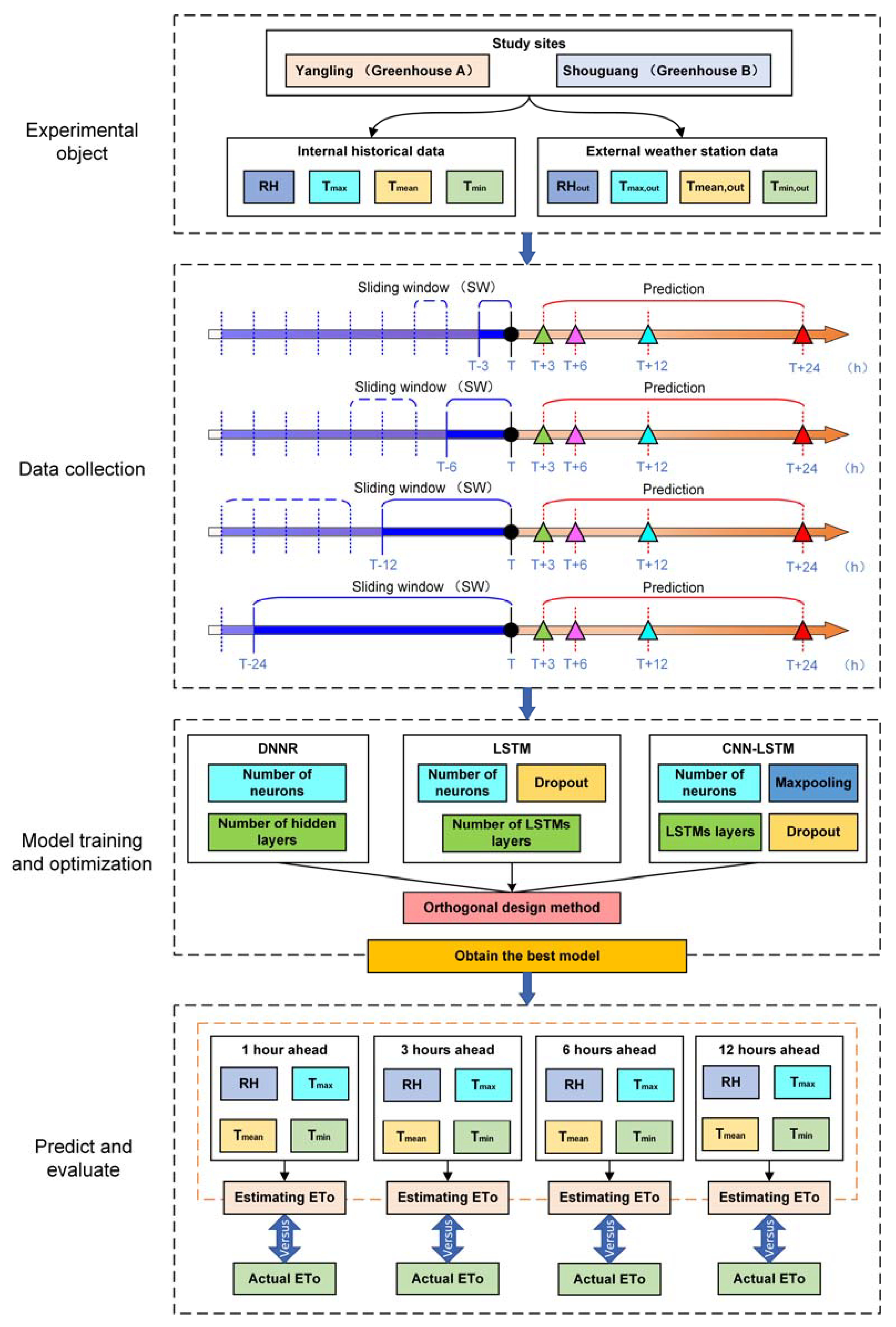
The overall research method of this study is sown in Figure 8, which includes experimental, data collection, model training and optimization, prediction, and evaluate. First, the outdoor meteorological data from the nearest weather station and the historical indoor weather data from two solar greenhouses were collected, the training set of each experiment was divided by four sliding windows (T-3h, T-6h, T-12h, and T-24h), and the test set of each best experiment was also divided by four sliding windows (T+3h, T+6h, T+12h, and T+24h), a total of 16 training sets and the corresponding test sets were generated, the sequence number and division methods of each combination of training set and the corresponding test set are shown in

Table 6. The sequence number and division methods of each combination of training set and corresponding test set.

Number	Training Set	Test Set	Number	Training Set	Test Set
No. 1	T-3h~T-1h	T+3h	No. 9	T-3h~T-1h	T+12h
No. 2	T-6h~T-1h		No. 10	T-6h~T-1h
No. 3	T-12h~T-1h		No. 11	T-12h~T-1h
No. 4	T-24h~T-1h		No. 12	T-24h~T-1h
No. 5	T-3h~T-1h	T+6h	No. 13	T-3h~T-1h	T+24h
No. 6	T-6h~T-1h		No. 14	T-6h~T-1h
No. 7	T-12h~T-1h		No. 15	T-12h~T-1h
No. 8	T-24h~T-1h		No. 16	T-24h~T-1h

.

Secondly, we developed three deep models of DNNR, LSTM and CNN-LSTM, in order to improve the efficiency of model training, the combination of hyperparameters for three models were generated using the orthogonal design, respectively. For three different types of models, each experimental model designed by orthogonal experiments was trained and tested 16 times in 16 datasets. For the DNNR, LSTM and CNN-LSTM models, we obtained the training results for 144, 144, and 288 experimental models, respectively.

4. Results and Discussion

This section provides a comparison of the prediction performance for three models, optimal forecast results at four forecast time points, and daily ET_o evaluated using the predicted environmental parameters.

4.1. Comparison of the Prediction Performance for Three Models

In order to verify the applicability of three models, each of nine DNNR models, nine LSTM models, and 18 CNN-LSTM models were trained and tested using 16 training sets and corresponding test sets. For three models, the best performing models of each training set and the corresponding test set are shown in

Table 7. The best performing models of each training set and corresponding test set.

Model Type	Number	Greenhouse A		Greenhouse B
		Humidity	Humidity	Temperature	Humidity
DNNR	No. 1	DNNR 8	DNNR 9	DNNR 5	DNNR 5
	No. 2	DNNR 5	DNNR 4	DNNR 5	DNNR 2
	No. 3	DNNR 9	DNNR 9	DNNR 6	DNNR 6
	No. 4	DNNR 4	DNNR 9	DNNR 3	DNNR 2
	No. 5	DNNR 1	DNNR 4	DNNR 4	DNNR 4
	No. 6	DNNR 6	DNNR 9	DNNR 6	DNNR 8
	No. 7	DNNR 9	DNNR 9	DNNR 4	DNNR 3
	No. 8	DNNR 9	DNNR 2	DNNR 2	DNNR 4
	No. 9	DNNR 9	DNNR 4	DNNR 6	DNNR 5
	No. 10	DNNR 8	DNNR 2	DNNR 6	DNNR 9
	No. 11	DNNR 8	DNNR 6	DNNR 5	DNNR 8
	No. 12	DNNR 8	DNNR 2	DNNR 9	DNNR 6
	No. 13	DNNR 8	DNNR 3	DNNR 3	DNNR 8
	No. 14	DNNR 4	DNNR 2	DNNR 6	DNNR 8
	No. 15	DNNR 6	DNNR 9	DNNR 8	DNNR 8
	No. 16	DNNR 5	DNNR 9	DNNR 5	DNNR 8
LSTM	No. 1	LSTM 7	LSTM 8	LSTM 7	LSTM 2
	No. 2	LSTM 8	LSTM 2	LSTM 7	LSTM 4
	No. 3	LSTM 9	LSTM 1	LSTM 3	LSTM 4
	No. 4	LSTM 1	LSTM 8	LSTM 8	LSTM 8
	No. 5	LSTM 8	LSTM 8	LSTM 7	LSTM 3
	No. 6	LSTM 3	LSTM 4	LSTM 9	LSTM 9
	No. 7	LSTM 7	LSTM 2	LSTM 4	LSTM 6
	No. 8	LSTM 8	LSTM 4	LSTM 2	LSTM 4
	No. 9	LSTM 4	LSTM 3	LSTM 4	LSTM 3
	No. 10	LSTM 8	LSTM 5	LSTM 4	LSTM 3
	No. 11	LSTM 9	LSTM 8	LSTM 7	LSTM 3
	No. 12	LSTM 8	LSTM 8	LSTM 1	LSTM 1
	No. 13	LSTM 4	LSTM 4	LSTM 2	LSTM 6
	No. 14	LSTM 1	LSTM 1	LSTM 6	LSTM 8
	No. 15	LSTM 5	LSTM 5	LSTM 7	LSTM 1
	No. 16	LSTM 1	LSTM 1	LSTM 4	LSTM 8
CNN-LSTM	No. 1	CNN-LSTM 1	CNN-LSTM 16	CNN-LSTM 4	CNN-LSTM 1
	No. 2	CNN-LSTM 15	CNN-LSTM 18	CNN-LSTM 15	CNN-LSTM 12
	No. 3	CNN-LSTM 12	CNN-LSTM 1	CNN-LSTM 12	CNN-LSTM 12
	No. 4	CNN-LSTM 2	CNN-LSTM 3	CNN-LSTM 8	CNN-LSTM 9
	No. 5	CNN-LSTM 16	CNN-LSTM 11	CNN-LSTM 1	CNN-LSTM 1
	No. 6	CNN-LSTM 11	CNN-LSTM 14	CNN-LSTM 2	CNN-LSTM 14
	No. 7	CNN-LSTM 14	CNN-LSTM 12	CNN-LSTM 3	CNN-LSTM 18
	No. 8	CNN-LSTM 13	CNN-LSTM 18	CNN-LSTM 8	CNN-LSTM 14
	No. 9	CNN-LSTM 11	CNN-LSTM 1	CNN-LSTM 11	CNN-LSTM 7
	No. 10	CNN-LSTM 11	CNN-LSTM 15	CNN-LSTM 6	CNN-LSTM 1
	No. 11	CNN-LSTM 17	CNN-LSTM 2	CNN-LSTM 3	CNN-LSTM 1
	No. 12	CNN-LSTM 5	CNN-LSTM17	CNN-LSTM 10	CNN-LSTM 17
	No. 13	CNN-LSTM 14	CNN-LSTM 4	CNN-LSTM 16	CNN-LSTM 1
	No. 14	CNN-LSTM 13	CNN-LSTM 18	CNN-LSTM 11	CNN-LSTM 8
	No. 15	CNN-LSTM 13	CNN-LSTM 6	CNN-LSTM 12	CNN-LSTM 10
	No. 16	CNN-LSTM 6	CNN-LSTM 9	CNN-LSTM 7	CNN-LSTM 16

. As can be seen from the table, the best performing DNNR model for different training and test sets is also different, and it is difficult to find the distribution rule of the best model for 16 datasets. The same conclusion applies to the LSTM and CNN-LSTM models. For humidity and temperature in two solar greenhouses, the best performing DNNR model for same training and test set is also different, the same conclusion applies to two greenhouses and the LSTM, CNN-LSTM models.

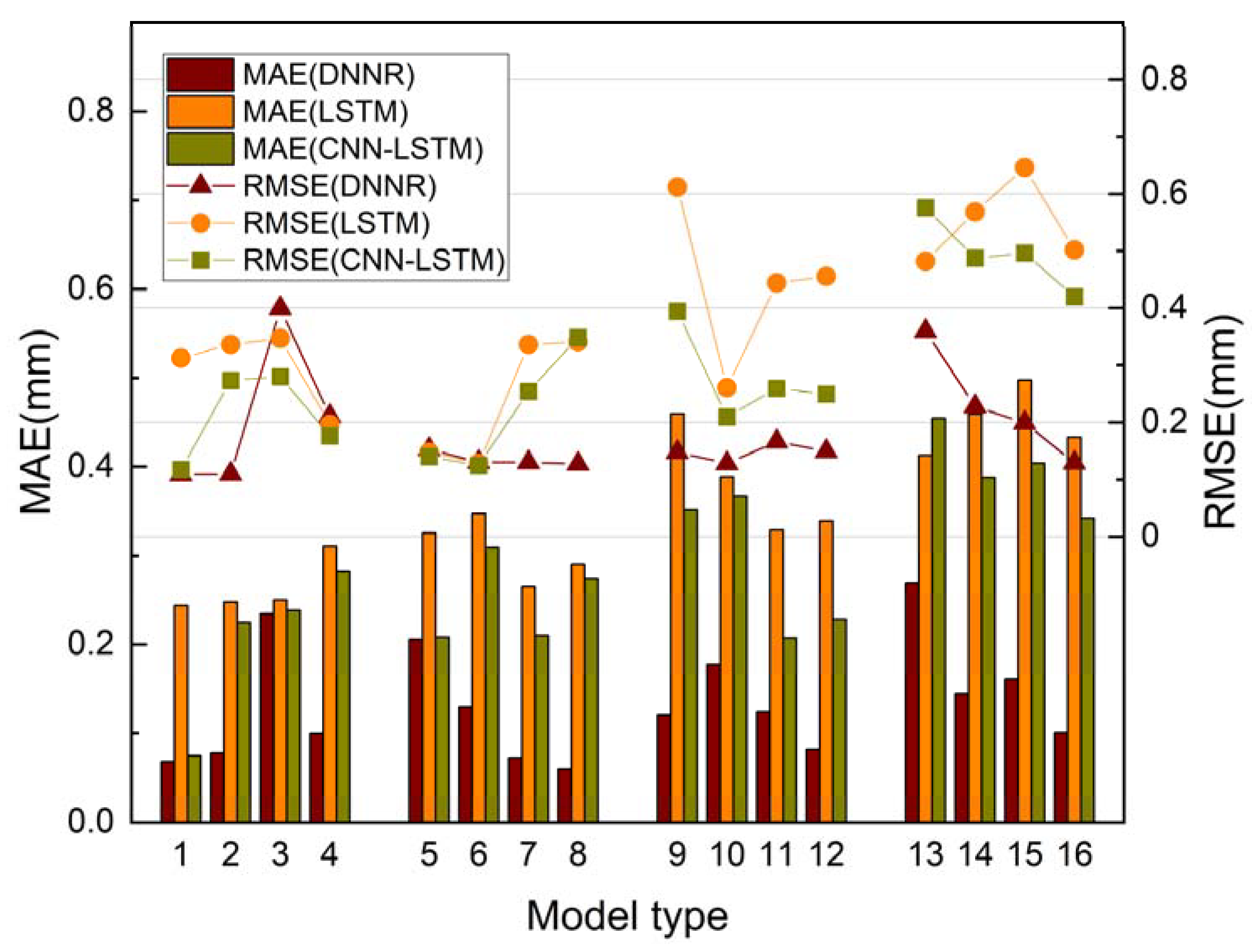
For three type prediction models of Greenhouse A humidity, the RMSE and MAE of the best experimental model in 16 datasets were shown in Figure 9, it can be seen from the results, for the test set of T+3h, T+12h and T+24h, the RMSE and MAE of the best LSTM and CNN-LSTM models increase with the training set time horizon, conversely, the RMSE and MAE of the best DNNR models decrease with the training set time horizon. For the test set of T+6h, the RMSE and MAE of the best LSTM and CNN-LSTM models decrease with the training set time horizon, conversely, the RMSE and MAE of the best DNNR models increases with the training set time horizon. In general, the MAE and RMSE of the best three models increase with the extension of forecast time, and the performance of DNNR was best among the three models.

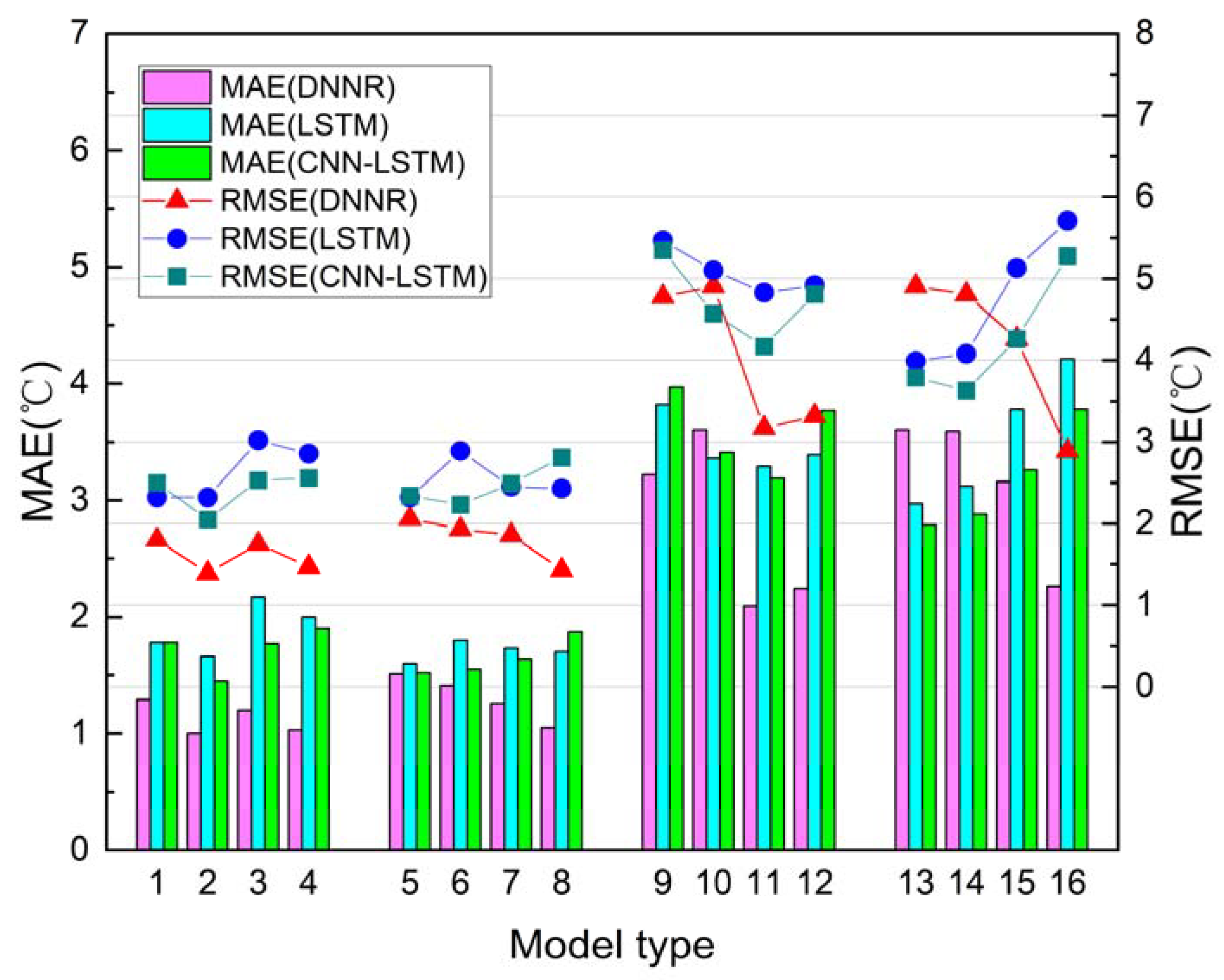
For three type prediction models of Greenhouse A temperature, the RMSE and MAE of the best experimental model under 16 datasets were shown in Figure 10, it can be seen from the results, for the test set of T+3h, T+6h and T+24h, the RMSE and MAE of the best LSTM and CNN-LSTM models increase with the training set time horizon. For the test set T+12h, the RMSE and MAE of the best LSTM and CNN-LSTM models decrease with the training set time horizon. Conversely, for the test set of T+3h, T+6h, T+12h and T+24h, the RMSE and MAE of the best DNNR models decrease with the training set time horizon. In general, the MAE and RMSE of the best three models also increases with the extension of forecast time, the performance of DNNR was also best among the three models.

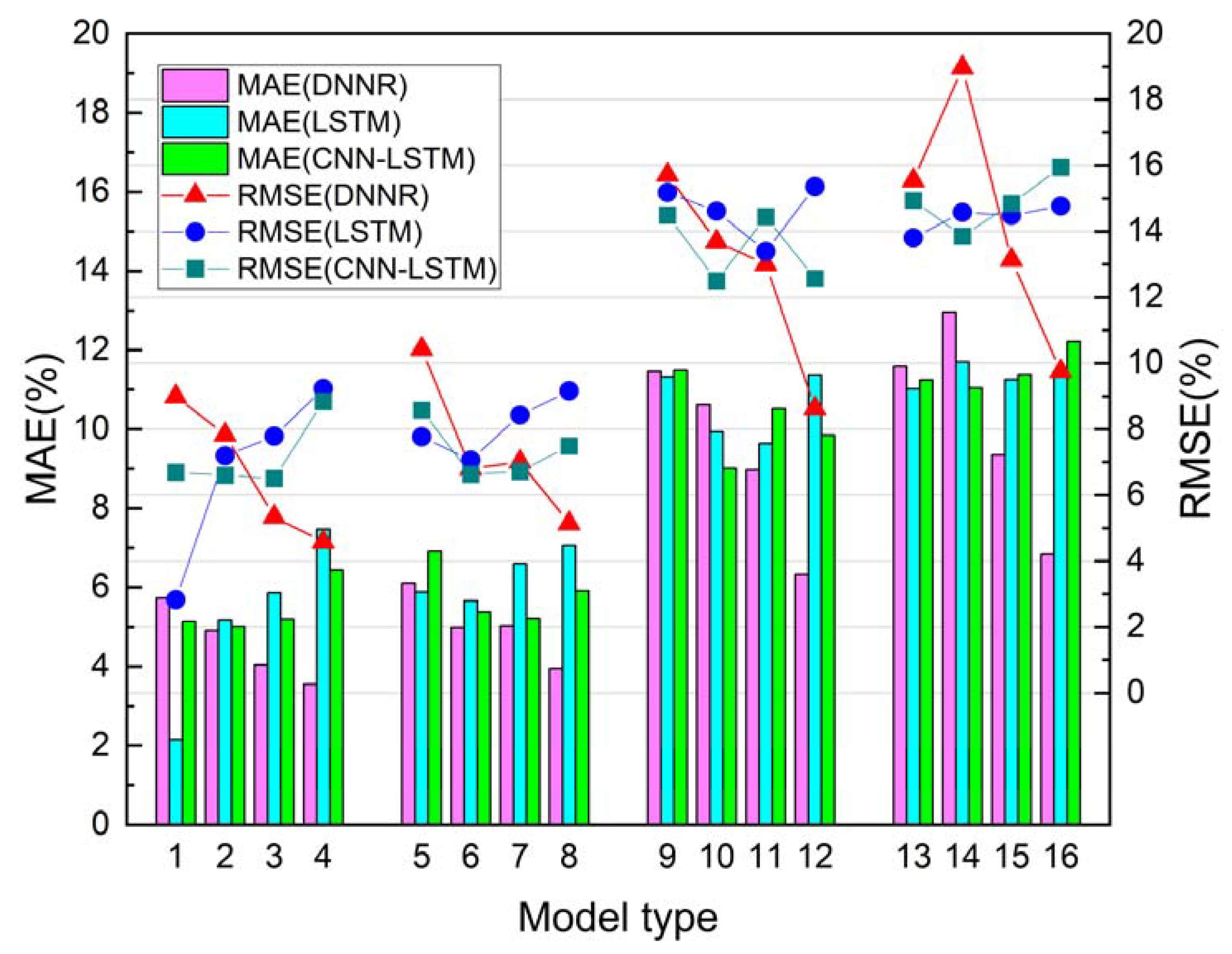
For three type prediction models of Greenhouse B humidity, the RMSE and MAE of the best experimental model in 16 datasets are shown in Figure 11, it can be seen from the results, for the test set of T+3h, T+6h and T+24h, the RMSE and MAE of the best LSTM and CNN-LSTM models increases with the training set time horizon. For test set T+12h, the RMSE and MAE of the best LSTM and CNN-LSTM models decrease with the training set time horizon. On the contrary, for the test set of T+3h, T+6h, T+12h and T+24h, the RMSE and MAE of the best DNNR models decrease with the training set time horizon. In general, the MAE and RMSE of the best three models also increases with the extension of the forecast time, and the performance of DNNR was also best among the three models.

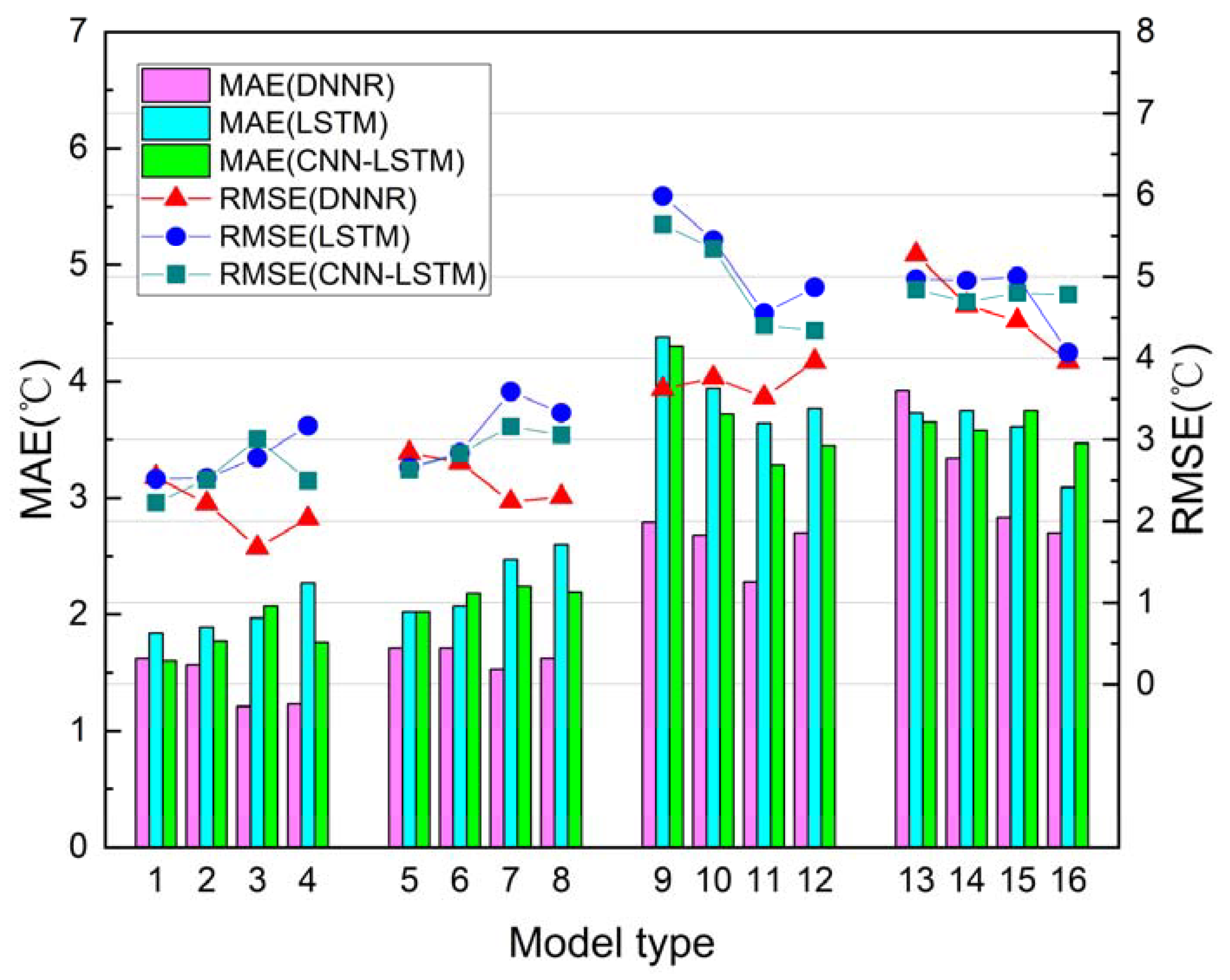
For three type prediction models of Greenhouse B temperature, the RMSE and MAE of the best experimental model in 16 datasets are shown in Figure 12, it can be seen from the results, for the test set of T+3h and T+6h, the RMSE and MAE of the best LSTM and CNN-LSTM models increases with the training set time horizon. For the test set of T+12h and T+24h, the RMSE and MAE of the best LSTM and CNN-LSTM models decrease with the training set time horizon. On the contrary, for the test set of T+3h, T+6h, T+12h and T+24h, the RMSE and MAE of the best DNNR models decrease with the training set time horizon. For the of T+12h test set, the RMSE and MAE of the best DNNR models increase with the training set time horizon. In general, the MAE and RMSE of the best three models are also increased with the extension of forecast time, the performance of DNNR was also the best among the three models.

4.2. Optimal Forecast Results at Four Forecast Time Points

For each forecast time points (T+3h, T+6h, T+12h and T+24h), the predictive performances of all experimental models were compared, and the best model at each forecast time point was shown in

Table 8. The best performing models at each forecast time point.

Greenhouse	Parameters	Models Type	Forecast Time Points
			T+3h	T+6h	T+12h	T+24h
Greenhouse A	Humidity	DNNR	No. 4	No. 8	No. 12	No. 16
		LSTM	No. 3	No. 7	No. 11	No. 13
		CNN-LSTM	No. 2	No. 8	No. 10	No. 13
	Temperature	DNNR	No. 2	No. 8	No. 11	No. 16
		LSTM	No. 2	No. 8	No. 11	No. 13
		CNN-LSTM	No. 2	No. 5	No. 11	No. 13
Greenhouse B	Humidity	DNNR	No. 4	No. 8	No. 12	No. 16
		LSTM	No. 1	No. 6	No. 10	No. 13
		CNN-LSTM	No. 2	No. 7	No. 12	No. 14
	Temperature	DNNR	No. 3	No. 7	No. 11	No. 16
		LSTM	No. 1	No. 5	No. 11	No. 16
		CNN-LSTM	No. 4	No. 5	No. 11	No. 16

; for Greenhouse A temperature prediction, the best models for each of the three different models are similar at each forecast time point. At the same time, for other parameters in two greenhouses, the best model for each of the three different models was not exactly the same at each forecast time point.

For the humidity of Greenhouse A, the statistics of the error distribution between the predicted value of the best model and the actual value at four forecast time points are shown in Figure 13. From the figure, the errors of the predictions of the DNNR model at four forecast time points are within [−8, 10], [−12, 13], [−44, 49] and [−19, 26], respectively. The errors of LSTM model predictions at four forecast time points are within [−19, 8], [−22, 13], [−26, 45] and [−41, 34], respectively. The errors of CNN-LSTM model predictions at four forecast time points are within [−21, 16], [−25, 18], [−28, 41] and [−31, 34], respectively. The errors of the three models increase with the prediction time, specifically, for the forecast time of T+12, the errors of the LSTM and CNN-LSTM models are smaller than the DNNR models, for the forecast time of T+3, T+6 and T+24, the errors of the DNNR model are smaller than the LSTM and CNN-LSTM models.

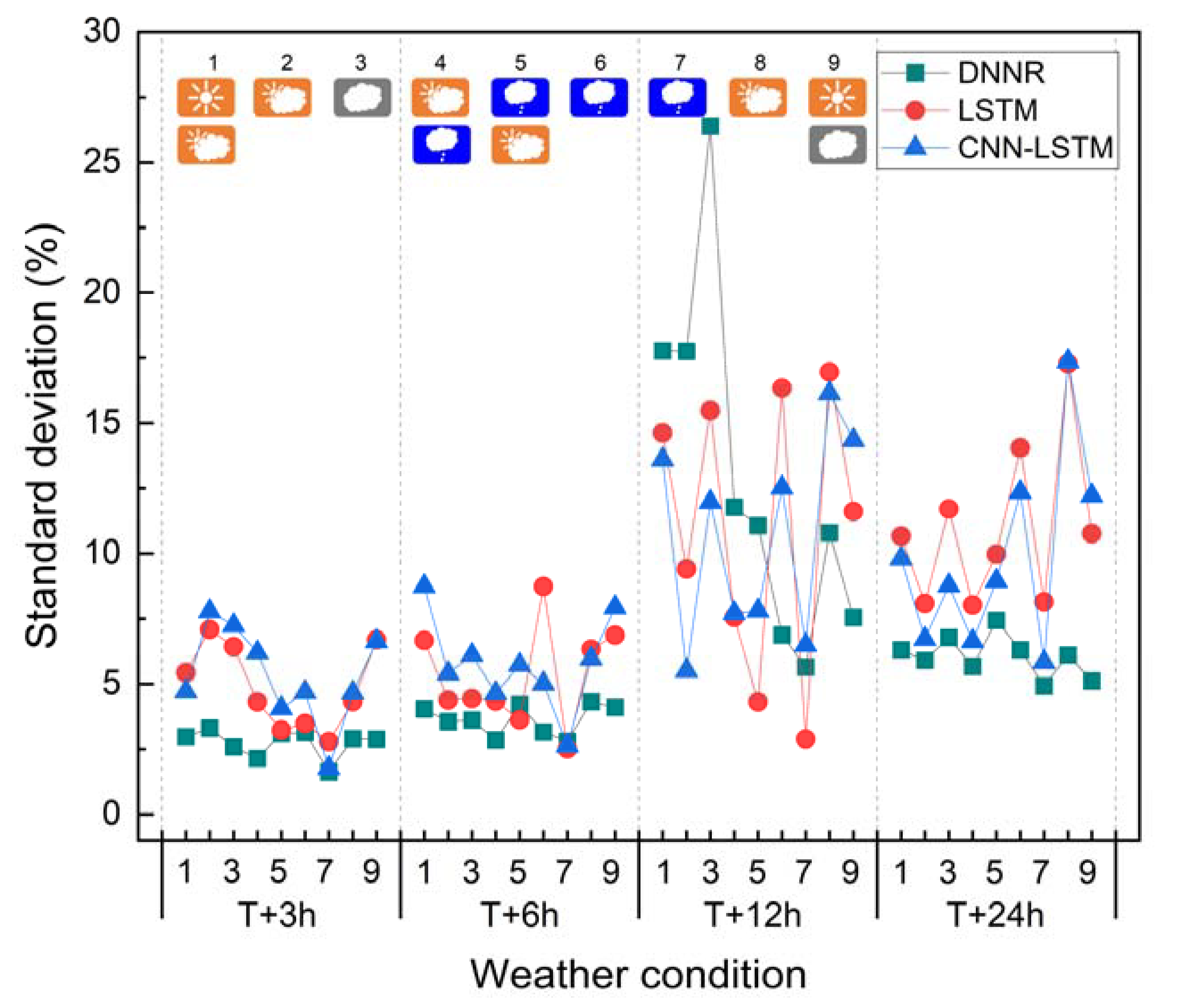
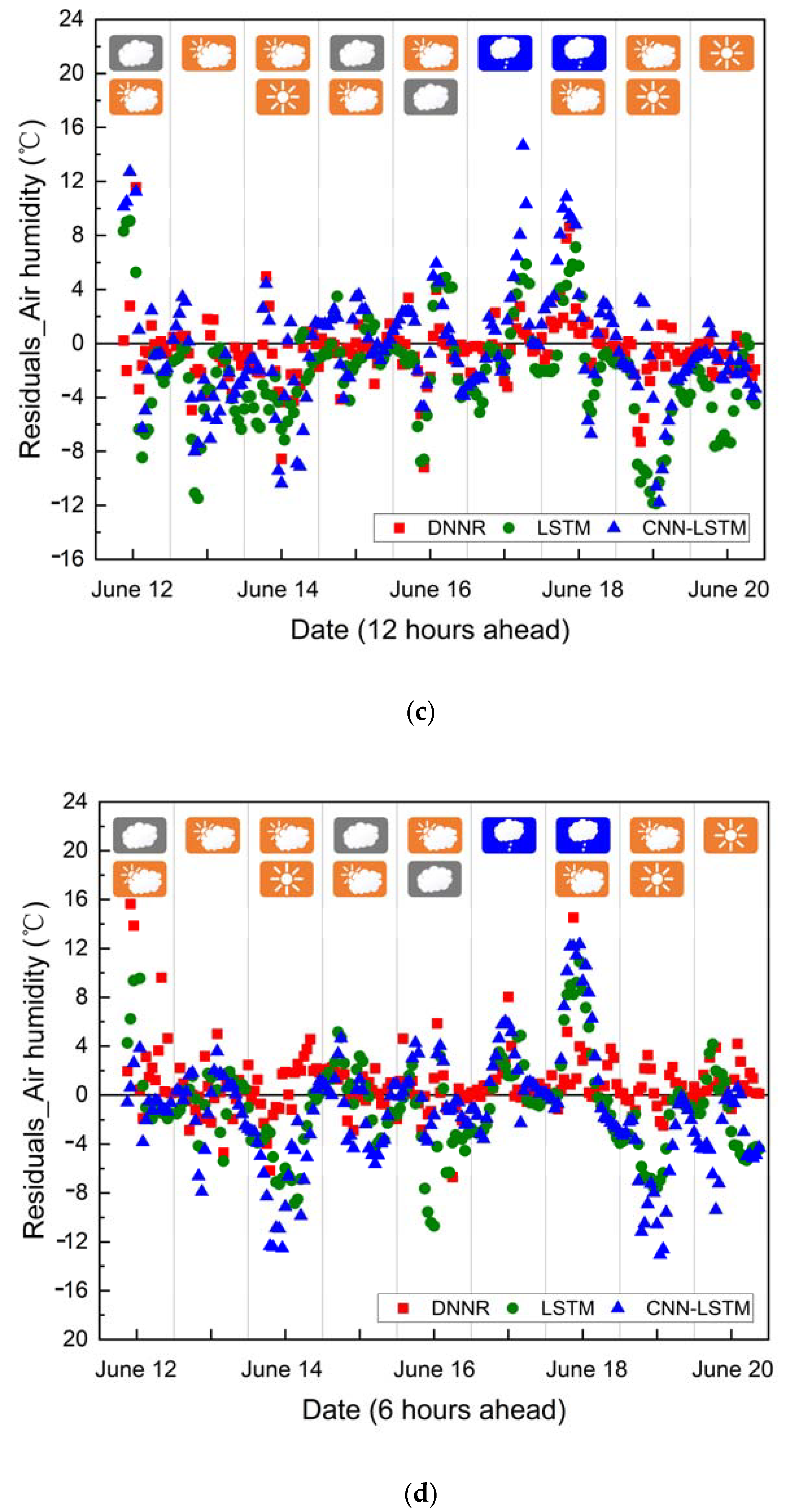
In order to analyze the correlation between the errors of the three forecasting models and the weather conditions, for the humidity of Greenhouse A, the ST of the three model errors under different weather conditions are shown in Figure 14; for three models, the ST of the DNNR model was the smallest under different weather conditions, and the ST of three models increase with the training set time horizon, the ST of three models are the largest at T+12 time point under different weather conditions, which means that the DNNR was the best predictive model among the three models, and the DNNR model was not suitable for parameter prediction 12 h ahead.

For the temperature of Greenhouse A, the statistics of the error distribution between the predicted value of the best model and the actual value at four forecast time points are shown in Figure 15. From the figure, the errors of the predictions of the DNNR model at four forecast time points are within [−5, 8], [−6, 6], [−8, 12] and [−7, 7] °C, respectively. The errors of LSTM model predictions at four forecast time points are within [−6, 9], [−6, 10], [−18, 17] and [−13, 11] °C, respectively. The errors in the predictions of the CNN-LSTM model at four forecast time points are within [−4, 7], [−3, 9], [−14, 12] and [−15, 8] °C, respectively. The errors of the three models increase with the prediction time, specifically, for the forecast time of T+12, the errors of the LSTM and CNN-LSTM models are also smaller than the DNNR models. For the forecast time of T+3, T+6 and T+24, the errors of the DNNR model are smaller than the LSTM and CNN-LSTM models.

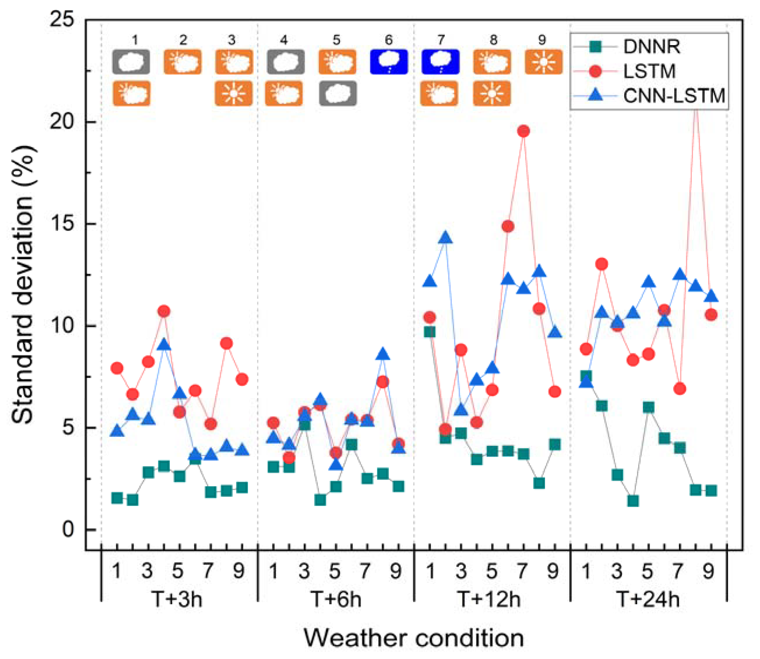
The ST of the errors of the three models under different weather conditions are shown in Figure 16, for three models, the ST of the DNNR model is also the smallest under different weather conditions, and the ST of three models increase with the training set time horizon, the ST of three models are the biggest at T+12 time point under different weather conditions, which means that the DNNR was the best predictive model among the three models, and the DNNR model was not suitable for parameters prediction 12 h ahead.

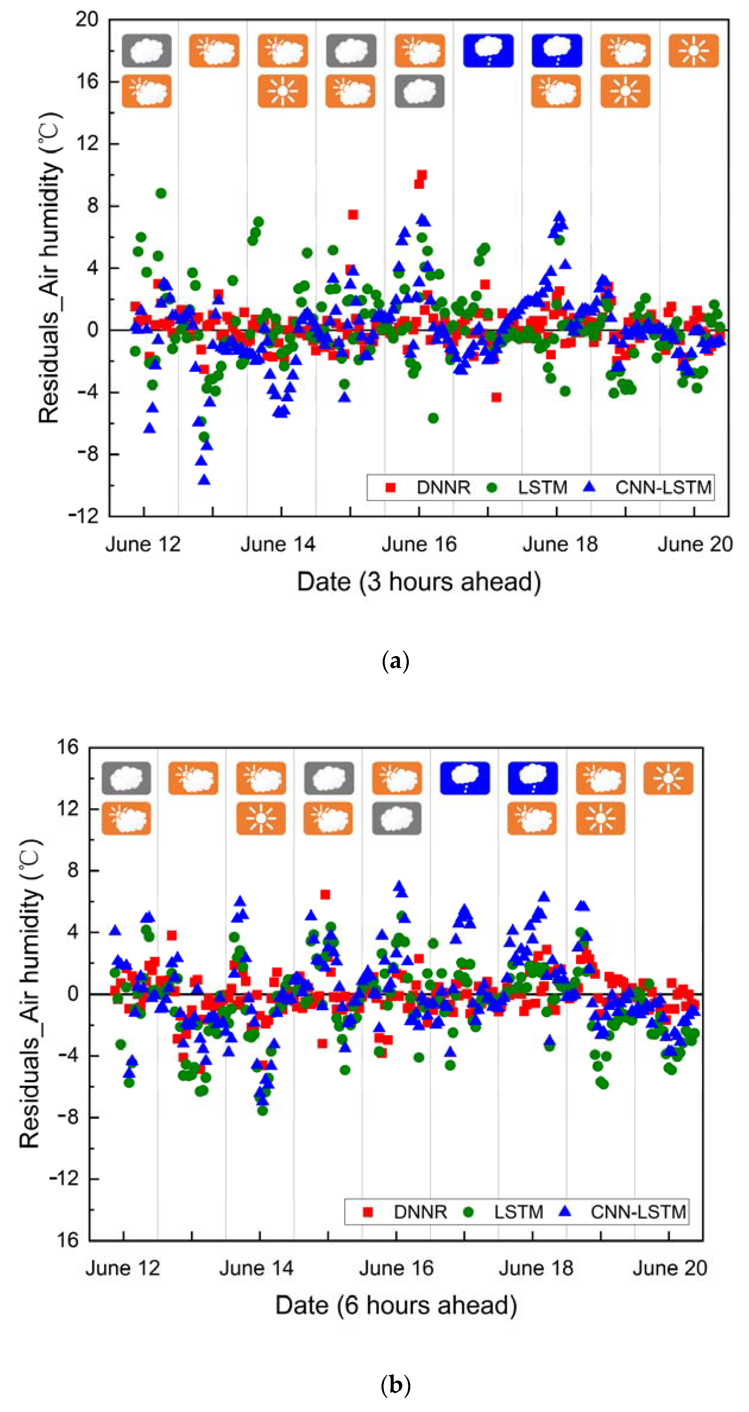
For Greenhouse B humidity, statistics of the error distribution between the predicted value of the best model and the actual value at four forecast time points are shown in Figure 17. From the figure, the errors of the predictions of the DNNR model at four forecast time points are within [−11, 6], [−13, 10], [−19, 23] and [−25, 27] %, respectively. The errors of the LSTM model predictions at four forecast time points are within [−29, 17], [−21, 9], [−51, 23] and [−37, 41] %, respectively. The errors of CNN-LSTM model predictions at four forecast time points are within [−28, 21], [−26, 9], [−44, 24] and [−37, 39] %, respectively. The errors of the three models increase with the prediction time, specifically, for the forecast time of T+12, the errors of the LSTM and CNN-LSTM models are smaller than the DNNR models, for the forecast time of T+3, T+6 and T+24, the errors of DNNR model are smaller than the LSTM and CNN-LSTM models.

The errors of the three models errors under different weather conditions are shown in Figure 18, for three models, the ST of DNNR model is the smallest under different weather conditions, and the ST of three models increase with the training set time horizon, the ST of three models are the biggest at T+12 time point under different weather conditions, which means that the DNNR is the best predictive model among the three models, and the DNNR model is not suitable for prediction of parameters 12 h ahead.

For Greenhouse B temperature, statistics of the error distribution between the predicted value of the best model and the actual value at four forecast time points are shown in Figure 19. From the figure, the errors in the predictions of the DNNR model at four forecast time points are within [−5, 10], [−5, 7], [−10, 12] and [−7, 16] °C, respectively. The errors in the predictions of the LSTM model at four forecast time points are within [−7, 9], [−8, 6], [−12, 10] and [−11, 13] °C, respectively. The errors in the predictions of the CNN-LSTM model predictions at four forecast time points are within [−10, 8], [−7, 7], [−12, 15] and [−14, 13] °C, respectively. The errors of the three models increase with the prediction time, specifically, for the forecast time of T+12, the errors of the LSTM and CNN-LSTM models are also smaller than the DNNR models, For the forecast time of T+3, T+6 and T+24, the errors of the DNNR model are smaller than the LSTM and CNN-LSTM models.

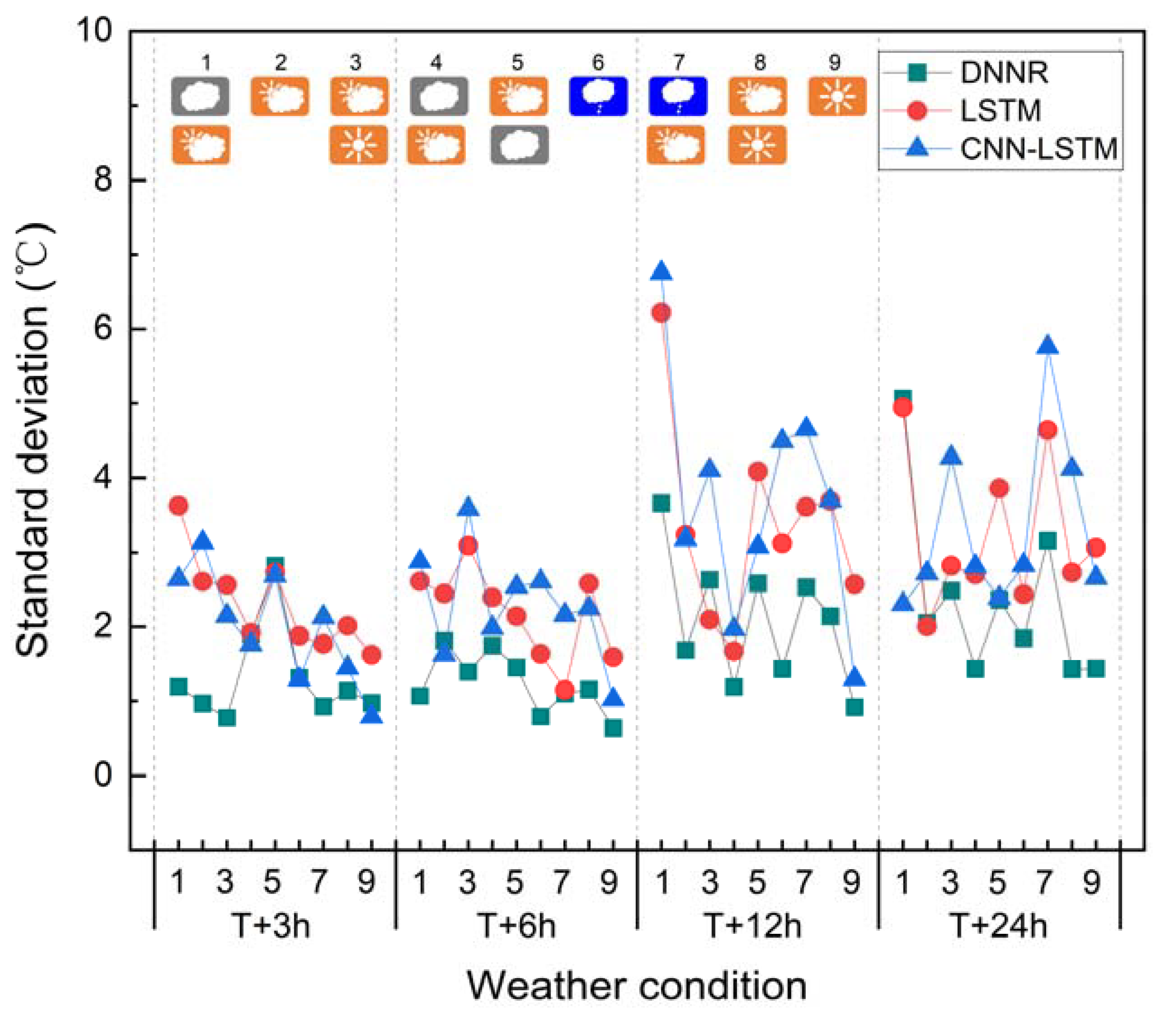
The ST of the errors of the three models under different weather conditions are shown in Figure 20, for three models, the ST of the DNNR model is also the smallest under different weather conditions, and the ST of three models increase with the training set time horizon, the ST of three models are the biggest at T+12 time point under different weather conditions, which means that the DNNR was the best predictive model among the three models, and the DNNR model was not suitable for parameter prediction 12 h ahead.

The degree of dispersion between the predictive value and the actual value of air humidity was larger than the degree of dispersion between the predictive value and the actual value of air temperature in two greenhouses, this was due to the greenhouse where the range of air humidity value was greater than the range of air temperature value.

4.3. Daily ET_o Evaluated Using the Predicted Environmental Parameters

For two solar greenhouses, the maximum and minimum air temperature in the solar greenhouse were predicted using the optimized temperature prediction model, respectively. Net radiation in two greenhouses was predicted by the sliding mean filtering method. By incorporating the above data into the PM formula, the hourly ET_o is calculated using the predictive maximum, minimum, and average air temperature, net radiation and RH, at the same time, the actual value of hourly ET_o was calculated using the monitored environmental parameters. Daily ET_o is obtained by accumulating hourly ET_o.

For the three models, the RMSE and MAE of the predicted daily ET_o and the actual daily ET_o for the Greenhouse A under four forecast time points are shown in Figure 21. It can be seen from the results, for the test set of T+3h, T+12h and T+24h, the RMSE and MAE of the best LSTM and CNN-LSTM models increase with the training set time horizon, and for the test set of T+6h, the RMSE and MAE of the best LSTM and CNN-LSTM models are decrease with the training set time horizon. On the contrary, for four forecast time points, the RMSE and MAE of the best DNNR models decrease with the training set time horizon. In general, the performance of DNNR was best among the three models.

The RMSE and MAE of the predicted daily ET_o and the actual daily ET_o for Greenhouse B under four forecast time points are shown in Figure 22. It can be seen from the results, for the test set of T+6h and T+24h, the RMSE and MAE of the best LSTM and CNN-LSTM models increase with the training set time horizon, and for the test set of T+6h and T+12h, the RMSE and MAE of the best LSTM and CNN-LSTM models are decrease with the training set time horizon. On the contrary, for four forecast time points, the RMSE and MAE of the best DNNR models decrease with the training set time horizon. In general, the performance of DNNR was best among the three models.

5. Discussion

The indoor temperature and relative humidity are keys to the healthy growth of solar greenhouse crops. In order to implement precise control and make irrigation decisions in advance, it is necessary to construct models to predict the indoor environmental parameters and ET_o [1,46]. Accurate prediction of indoor and outdoor environmental parameter and ET_o of solar greenhouses requires complete indoor and outdoor environmental parameters of the greenhouse.

Although many kinds of models have been developed for indoor environmental parameters of greenhouses, has all have their own drawbacks. Previously, Imran et al. [12] utilized artificial neural networks for the prediction of hourly mean values of ambient temperature. Morteza et al. [17] compared mathematical models with artificial neural network and select the best prediction models. Yu et al. [20] presented a novel temperature prediction model based on a least squares support vector machine model with parameters optimized by the improved particle swarm optimization. Yue et al. [18] proposed a model to predict the temperature and humidity of a greenhouse based on improved LM-RBF. Wang et al. [47] proposed the model of greenhouse temperature and parameter states. All these models mainly consider the environmental parameters inside the greenhouse and the change trend of time series. Jung et al. [8] proposed three deep learning models to predicting environmental parameters change. Although these models considering the external and indoor environmental parameters of the greenhouse, the prediction time steps are only from 5 to 30 min. Most of the indoor environmental parameters (air temperature and air humidity) of solar greenhouses in developing countries can be monitored completely and accurately [13,48]. Agricultural activities, especially crop production in greenhouse, are sensitive to the prediction time steps of the prediction model. Although in general, the shorter the prediction time, the higher the accuracy of the deep model, in the actual greenhouse crop irrigation decision and management process, the prediction time steps from 5 to 30 min are actually relatively short.

The outdoor environmental parameters monitored by small weather stations, due to the high cost of outdoor environmental parameter acquisition equipment and the small monitoring coverage, the environmental parameters prediction models using outdoor environmental parameters and indoor environmental parameters for solar greenhouses in China are still not entirely reliable, and a universal model has not yet been reported. In this study, three deep learning time series models were built, and the hyperparameters of these models were designed using the orthogonal design. In order to verify the precision of three models under long time steps, indoor and external environmental parameters from the nearest weather station were predicted using three models in 16 datasets, the optimized model was used to predict environmental parameters under four forecast time points, 3 h, 6 h, 12 h and 24 h, respectively. The results show that the DNNR model shows the best performance for the prediction of short-term greenhouse environmental parameters. The optimized models can help users realize prediction of water consumption without the recent environmental parameters of the solar greenhouse, which can reduce dependence of prediction of greenhouse crop water consumption on environmental detection sensors.

6. Conclusions

In order to predict the indoor environmental parameters of two solar greenhouses, this paper constructs three deep learning models (DNNR, LSTM and CNN-LSTM) for indoor environmental parameters forecast, the architecture and hyperparameters of three models were optimized using the orthogonal experimental design. The correlation between indoor environmental parameters and eight outdoor environmental parameters from the weather station was analyzed, and four parameters are selected as input of the prediction model.

Each of the three models were trained using the combination of indoor and weather station environmental parameters data set, and the models with the best predictive performance under four forecast time points are selected. Predictive performances of all experimental models were compared. For air temperature and humidity in two greenhouses, the errors of the three models increase with the prediction time, specifically, for the forecast time of T+12, the errors of the LSTM and CNN-LSTM models are smaller than the DNNR models, for the other three time points, the errors of the DNNR model are smaller than the LSTM and CNN-LSTM models. In general, the performance of DNNR was best among the three models.

The maximum and minimum temperature of the air were predicted using optimized temperature prediction models, and the RH_in of two solar greenhouses were also predicted. Based on the PM formula, the ET_o was calculated using five predictive environmental parameters. At the same time, the actual ET_o were calculated using the monitored environmental parameters. The results show that the DNNR model has excellent prediction accuracy. It is feasible to apply indoor environmental parameters and ET_o predictions with optimized models and provide technical support for irrigation strategies and drought control.

References

1. Guo, Y.; Zhao, H.; Zhang, S.; Wang, Y.; Chow, D. Modeling and optimization of environment in agricultural greenhouses for improving cleaner and sustainable crop production. J. Clean. Prod. 2021, 285, 124843. [Google Scholar] [CrossRef]
2. Zhang, M.; Yan, T.; Wang, W.; Jia, X.; Wang, J.; Klemeš, J.J. Energy-saving design and control strategy towards modern sustainable greenhouse: A review. Renew. Sustain. Energy Rev. 2022, 164, 112602. [Google Scholar] [CrossRef]
3. Zhang, X.; Gao, L.; Zhao, Z.; Ren, B. Modeling and analysis of greenhouse environmental factors in north China based on path analysis and stepwise regression. Semin. Ciências Agrárias 2020, 41, 2587–2596. [Google Scholar] [CrossRef]
4. Gharghory, S.M. Deep Network based on Long Short-Term Memory for Time Series Prediction of Microclimate Data inside the Greenhouse. Int. J. Comput. Intell. Appl. 2020, 19, 2050013. [Google Scholar] [CrossRef]
5. Altikat, S. Prediction of CO2 emission from greenhouse to atmosphere with artificial neural networks and deep learning neural networks. Int. J. Environ. Sci. Technol. 2021, 18, 3169–3178. [Google Scholar] [CrossRef]
6. Shen, Y.; Wei, R.; Xu, L. Energy Consumption Prediction of a Greenhouse and Optimization of Daily Average Temperature. Energies 2018, 11, 65. [Google Scholar] [CrossRef] [Green Version]
7. Villagran, E.; Leon, R.; Rodriguez, A.; Jaramillo, J. 3D Numerical Analysis of the Natural Ventilation Behavior in a Colombian Greenhouse Established in Warm Climate Conditions. Sustainability 2020, 12, 8101. [Google Scholar] [CrossRef]
8. Jung, D.-H.; Kim, H.S.; Jhin, C.; Kim, H.-J.; Park, S.H. Time-serial analysis of deep neural network models for prediction of climatic conditions inside a greenhouse. Comput. Electron. Agric. 2020, 173, 105402. [Google Scholar] [CrossRef]
9. Linge, Q.; Jin, D.; Shen, J.; Fu, Z.; Linge, N. A_WSN-based_prediction_model_of_microclimate_in_a_greenhouse_using_extreme_learning_approaches. ICACT Trans. Adv. Commun. Technol. 2015, 4, 6. [Google Scholar]
10. Ullah, I.; Fayaz, M.; Naveed, N.; Kim, D. ANN Based Learning to Kalman Filter Algorithm for Indoor Environment Prediction in Smart Greenhouse. IEEE Access 2020, 8, 159371–159388. [Google Scholar] [CrossRef]
11. Elbeltagi, A.; Azad, N.; Arshad, A.; Mohammed, S.; Mokhtar, A.; Pande, C.; Etedali, H.R.; Bhat, S.A.; Islam, A.R.M.T.; Deng, J. Applications of Gaussian process regression for predicting blue water footprint: Case study in Ad Daqahliyah, Egypt. Agric. Water Manag. 2021, 255, 107052. [Google Scholar] [CrossRef]
12. Tasadduq, I.; Rehman, S.; Bubshait, K. Application of neural networks for theprediction of hourly mean surface temperatures in Saudi Arabia. Renew. Energy 2002, 25, 10. [Google Scholar] [CrossRef]
13. Dai, W.; Wang, L.; Wang, B.; Cui, X.; Li, X. Research on WNN Greenhouse Temperature Prediction Method Based on GA. Phyton 2022, 91, 2283–2296. [Google Scholar] [CrossRef]
14. Ding, J.-T.; Tu, H.-Y.; Zang, Z.-L.; Huang, M.; Zhou, S.-J. Precise control and prediction of the greenhouse growth environment of Dendrobium candidum. Comput. Electron. Agric. 2018, 151, 453–459. [Google Scholar] [CrossRef]
15. Hernández-Morales, C.A.; Luna-Rivera, J.M.; Perez-Jimenez, R. Design and deployment of a practical IoT-based monitoring system for protected cultivations. Comput. Commun. 2022, 186, 51–64. [Google Scholar] [CrossRef]
16. Xu, Y.; Ji, R. Research on temperature prediction of intelligent greenhouse based on complex neural network. J. Chin. Agric. Mech. 2019, 40, 5. [Google Scholar]
17. Taki, M.; Ajabshirchi, Y.; Ranjbar, S.F.; Rohani, A.; Matloobi, M. Heat transfer and MLP neural network models to predict inside environment variables and energy lost in a semi-solar greenhouse. Energy Build. 2016, 110, 314–329. [Google Scholar] [CrossRef]
18. Yue, Y.; Quan, J.; Zhao, H.; Wang, H. The prediction of Greenhouse Temperature and Humidity Based on LM-RBF Network. In Proceedings of the 2018 IEEE International Conference on Mechatronics and Automation, Changchun, China, 5–8 August 2018; p. 5. [Google Scholar]
19. Yates, D.; Gangopadhyay, S.; Rajagopalan, B.; Strzepek, K. A technique for generating regional climate scenarios using a nearest-neighbor algorithm. Water Resour. Res. 2003, 39. [Google Scholar] [CrossRef] [Green Version]
20. Yu, H.; Chen, Y.; Hassan, S.G.; Li, D. Prediction of the temperature in a Chinese solar greenhouse based on LSSVM optimized by improved PSO. Comput. Electron. Agric. 2016, 122, 94–102. [Google Scholar] [CrossRef]
21. Elbeltagi, A.; Kumar, M.; Kushwaha, N.L.; Pande, C.B.; Ditthakit, P.; Vishwakarma, D.K.; Subeesh, A. Drought indicator analysis and forecasting using data driven models: Case study in Jaisalmer, India. Stoch. Environ. Res. Risk Assess. 2022. [Google Scholar] [CrossRef]
22. Elbeltagi, A.; Nagy, A.; Mohammed, S.; Pande, C.B.; Kumar, M.; Bhat, S.A.; Zsembeli, J.; Huzsvai, L.; Tamás, J.; Kovács, E.; et al. Combination of Limited Meteorological Data for Predicting Reference Crop Evapotranspiration Using Artificial Neural Network Method. Agronomy 2022, 12, 516. [Google Scholar] [CrossRef]
23. Kumar, M.; Elbeltagi, A.; Pande, C.B.; Ahmed, A.N.; Chow, M.F.; Pham, Q.B.; Kumari, A.; Kumar, D. Applications of Data-driven Models for Daily Discharge Estimation Based on Different Input Combinations. Water Resour. Manag. 2022, 36, 2201–2221. [Google Scholar] [CrossRef]
24. Alhnaity, B.; Pearson, S.; Leontidis, G.; Kollias, S. Using Deep Learning to Predict Plant Growth and Yield in Greenhouse Environments. Int. Soc. Hortic. Sci. 2020, 1296. [Google Scholar] [CrossRef]
25. Codeluppi, G.; Davoli, L.; Ferrari, G. Forecasting Air Temperature on Edge Devices with Embedded AI. Sensors 2021, 21, 3973. [Google Scholar] [CrossRef] [PubMed]
26. Liu, Y.; Li, D.; Wan, S.; Wang, F.; Dou, W.; Xu, X.; Li, S.; Ma, R.; Qi, L. A long short-term memory-based model for greenhouse climate prediction. Int. J. Intell. Syst. 2021, 37, 135–151. [Google Scholar] [CrossRef]
27. Bhat, S.A.; Huang, N.-F.; Hussain, I.; Bibi, F.; Sajjad, U.; Sultan, M.; Alsubaie, A.S.; Mahmoud, K.H. On the Classification of a Greenhouse Environment for a Rose Crop Based on AI-Based Surrogate Models. Sustainability 2021, 13, 12166. [Google Scholar] [CrossRef]
28. Lee, J.; Oh, J.; Cho, Y.; Lee, D. A Research about Time Domain Estimation Method for Greenhouse Environmental Factors based on Artificial Intelligence. Prot. Hortic. Plant Fact. 2020, 29, 277–284. [Google Scholar] [CrossRef]
29. Liang, H.; Hu, K.; Batchelor, W.D.; Chen, Q.; Liang, B.; Li, B. Modeling dissolved organic nitrogen dynamics under different N management practices for intensive greenhouse production using an improved WHCNS_veg model. Geoderma 2019, 337, 1039–1050. [Google Scholar] [CrossRef]
30. Temesgen, B.; Eching, S.; Davidoff, B.; Frame, K. Comparison of Some Reference Evapotranspiration Equations for California. J. Irrig. Drain. Eng. 2005, 131, 73–84. [Google Scholar] [CrossRef]
31. Incrocci, L.; Thompson, R.B.; Fernandez-Fernandez, M.D.; De Pascale, S.; Pardossi, A.; Stanghellini, C.; Rouphael, Y.; Gallardo, M. Irrigation management of European greenhouse vegetable crops. Agric. Water Manag. 2020, 242, 106393. [Google Scholar] [CrossRef]
32. Itenfisu, D.; Elliott, R.L.; Allen, R.G.; Walter, I.A. Comparison of Reference Evapotranspiration Calculations as Part of the ASCE Standardization Effort. J. Irrig. Drain. Eng. 2003, 129, 9. [Google Scholar] [CrossRef]
33. Merkel, G.; Povinelli, R.; Brown, R. Short-Term Load Forecasting of Natural Gas with Deep Neural Network Regression. Energies 2018, 11, 2008. [Google Scholar] [CrossRef]
34. Guo, C.; Cui, Y. Utilizing artificial neural network to simulate and predict the hydraulic performance of free water surface constructed wetlands. J. Environ. Manag. 2022, 305, 114334. [Google Scholar] [CrossRef] [PubMed]
35. Lu, C.; Jiang, H.; You, C.; Wang, Y.; Ma, K.; Li, J. A novel method to determine the thief zones in heavy oil reservoirs based on convolutional neural network. J. Pet. Sci. Eng. 2021, 201, 108471. [Google Scholar] [CrossRef]
36. Cai, Y.; Zheng, W.; Zhang, X.; Zhangzhong, L.; Xue, X. Research on soil moisture prediction model based on deep learning. PLoS ONE 2019, 14, e0214508. [Google Scholar] [CrossRef]
37. Parisi, L.; Ma, R.; RaviChandran, N.; Lanzillotta, M. hyper-sinh: An accurate and reliable function from shallow to deep learning in TensorFlow and Keras. Mach. Learn. Appl. 2021, 6, 100112. [Google Scholar] [CrossRef]
38. Meka, R.; Alaeddini, A.; Bhaganagar, K. A robust deep learning framework for short-term wind power forecast of a full-scale wind farm using atmospheric variables. Energy 2021, 221, 119759. [Google Scholar] [CrossRef]
39. Wang, S.; Li, P.; Ji, H.; Zhan, Y.; Li, H. Prediction of air particulate matter in Beijing, China, based on the improved particle swarm optimization algorithm and long short-term memory neural network. J. Intell. Fuzzy Syst. 2021, 41, 1869–1885. [Google Scholar] [CrossRef]
40. Song, X.; Liu, Y.; Xue, L.; Wang, J.; Zhang, J.; Wang, J.; Jiang, L.; Cheng, Z. Time-series well performance prediction based on Long Short-Term Memory (LSTM) neural network model. J. Pet. Sci. Eng. 2020, 186, 106682. [Google Scholar] [CrossRef]
41. Deo, R.C.; Grant, R.H.; Webb, A.; Ghimire, S.; Igoe, D.P.; Downs, N.J.; Al-Musaylh, M.S.; Parisi, A.V.; Soar, J. Forecasting solar photosynthetic photon flux density under cloud cover effects: Novel predictive model using convolutional neural network integrated with long short-term memory network. Stoch. Environ. Res. Risk Assess. 2022, 36, 3183–3220. [Google Scholar] [CrossRef]
42. Wu, L.; Dong, Z.; Li, W.; Jing, C.; Qu, B. Well-Logging Prediction Based on Hybrid Neural Network Model. Energies 2021, 14, 8583. [Google Scholar] [CrossRef]
43. Agga, A.; Abbou, A.; Labbadi, M.; Houm, Y.E.; Ou Ali, I.H. CNN-LSTM: An efficient hybrid deep learning architecture for predicting short-term photovoltaic power production. Electr. Power Syst. Res. 2022, 208, 107908. [Google Scholar] [CrossRef]
44. Eren, L.; Ince, T.; Kiranyaz, S. A Generic Intelligent Bearing Fault Diagnosis System Using Compact Adaptive 1D CNN Classifier. J. Signal Process. Syst. 2018, 91, 179–189. [Google Scholar] [CrossRef]
45. Lin, K.; Tian, L.; Zhao, Y.; Zhao, C.; Zhang, M.; Zhou, T. Pyrolytic characteristics of fine materials from municipal solid waste using TG-FTIR, Py-GC/MS, and deep learning approach: Kinetics, thermodynamics, and gaseous products distribution. Chemosphere 2022, 293, 133533. [Google Scholar] [CrossRef] [PubMed]
46. Liu, R.; Li, M.; Guzmán, J.L.; Rodríguez, F. A fast and practical one-dimensional transient model for greenhouse temperature and humidity. Comput. Electron. Agric. 2021, 186, 106186. [Google Scholar] [CrossRef]
47. Wang, L.; Wang, B. Construction of greenhouse environment temperature adaptive model based on parameter identification. Comput. Electron. Agric. 2020, 174, 105477. [Google Scholar] [CrossRef]
48. Wang, L.; Wang, B.; Zhu, M. Multi-Model Adaptive Fuzzy Control System Based on Switch Mechanism in a Greenhouse. Appl. Eng. Agric. 2020, 36, 549–556. [Google Scholar] [CrossRef]
Figure 1. Schematic diagram of experimental solar greenhouses.
Applsci 12 12529 g001
Figure 2. Timing diagram of environmental parameters in the Greenhouse A. (a) Average humidity of the air every hour and (b) temperature.
Applsci 12 12529 g002
Figure 3. Timing diagram of environment parameters of Greenhouse B. (a) Average humidity of the air every hour and (b) temperature.
Applsci 12 12529 g003
Figure 4. The frame of the DNNR network for regression problems.
Applsci 12 12529 g004
Figure 5. The basic LSTM network architecture for regression problems.
Applsci 12 12529 g005
Figure 6. The frame of the LSTM network for regression problems.
Applsci 12 12529 g006
Figure 7. The frame of the CNN-LSTM network for regression problems.
Applsci 12 12529 g007
Figure 8. The overview of the research in this paper.
Applsci 12 12529 g008
Figure 9. The RMSE and MAE of the best experimental model for Greenhouse A humidity under 16 datasets.
Applsci 12 12529 g009
Figure 10. The RMSE and MAE of the best experimental model for Greenhouse A temperature under 16 datasets.
Applsci 12 12529 g010
Figure 11. The RMSE and MAE of the best experimental model for Greenhouse B humidity under 16 datasets.
Applsci 12 12529 g011
Figure 12. The RMSE and MAE of the best experimental model for Greenhouse B temperature under 16 datasets.
Applsci 12 12529 g012
Figure 13. Statistics of the error distribution between the predicted value of the best model and the actual value for the humidity of Greenhouse A.
Applsci 12 12529 g013
Figure 14. The ST of the three model errors for Greenhouse A humidity under different weather conditions; (a) 3 h advance, (b) 6 h advance, (c) 12 h advance, (d) 24 h advance.
Applsci 12 12529 g014aApplsci 12 12529 g014b
Figure 15. Statistics of the error distribution between the predicted value of the best model and the actual value for the humidity of Greenhouse A.
Applsci 12 12529 g015
Figure 16. The ST of the three model errors for Greenhouse A temperature under different weather conditions; (a) 3 h advance, (b) 6 h advance, (c) 12 h advance, (d) 24 h advance.
Applsci 12 12529 g016aApplsci 12 12529 g016b
Figure 17. Statistics of the error distribution between the predicted value of the best model and the actual value for Greenhouse B humidity.
Applsci 12 12529 g017
Figure 18. The ST of the three model errors for Greenhouse B humidity under different weather conditions; (a) 3 h advance, (b) 6 h advance, (c) 12 h advance, (d) 24 h advance.
Applsci 12 12529 g018aApplsci 12 12529 g018b
Figure 19. The statistics of the error distribution between the predicted value of the best model and the actual value for Greenhouse B temperature.
Applsci 12 12529 g019
Figure 20. The ST of the three model errors for Greenhouse B temperature under different weather conditions; (a) 3 h advance, (b) 6 h advance, (c) 12 h advance, (d) 24 h advance.
Applsci 12 12529 g020aApplsci 12 12529 g020b
Figure 21. The RMSE and MAE of predictive daily ETo and actual ETo for Greenhouse A under four forecast time points.
Applsci 12 12529 g021
Figure 22. The RMSE and MAE of predictive daily ETo and actual ETo for Greenhouse B under four forecast time points.
Applsci 12 12529 g022