AUV Drift Track Prediction Method Based on a Modified Neural Network

Abstract

Since AUV works in the complex marine environment without cable and unmanned, there will be a loss of contact when an accident occurs. It is necessary to carry out research on the drift track prediction of AUV for the sake of salvage and recovery of the AUV in time. It is worth noting that the volume of AUV is small, and the drift track changes significantly when it is affected by the marine environment. Consequently, when the AUV drifts to different ocean layers, there will be a feature drift problem which will lead to a significant drop in the prediction accuracy. In this paper, a new method of AUV drift track prediction is proposed. Inspired by the human emotion modulation mechanism in psychology, a modified neural network (ECRNet) is proposed to correct the prediction error in different ocean layers. Through experimental verification, the network reduces the prediction error and achieves a better prediction performance.

1. Introduction

AUV plays an important and irreplaceable role in ocean development and coastal defense due to its characteristics of small size, low noise, and flexibility [1,2]. However, AUVs will lose control and contact in the process of performing tasks for the immature cognition of the complex marine environment and equipment. Consequently, it is necessary to help rescue AUVs in a timely way and research the causes of failure through predicting drift track quickly and accurately. The prediction of the AUV drift track is mainly divided into two methods. One is based on the method of solving the dynamic equation. However, the influence of the marine environment on the drift motion of the AUV is random, which makes the process of establishing the equation complex and difficult to achieve. The other is based on data statistics and artificial intelligence methods [3].

The AUV rises slowly under the action of residual buoyancy after the outing of control at a great diving depth. At the same time, it drifts horizontally under the action of ocean factors such as current and wave. The motion research of the underwater robot under the interaction of current, wave, and other factors is of great interest in the community. Liu et al. [4] proposed a continuous finite time tracking control scheme based on the piecewise function modified nonsingular terminal sliding surface by studying the trajectory shift of the AUV under the action of ocean current and waves to make the tracking error converge to the minimum region of zero in a fixed time. Gao Z et al. [5] also studied the formation tracking control performance of the AUV with the combination of external disturbances caused by wind, wave, and current and model parameter uncertainty to improve the model parameter uncertainty and external disturbances. Byrne [6] simulated the complex marine environment outside the Phoenix AUV virtual world and the interaction between the physical model and the AUV in real time. Gabl et al. [7,8] investigated the forces imparted by currents (with representative real-world turbulence) and waves on a commercially available ROV, and the provided dataset can be used as a validation experiment as well as for testing and development of an algorithm for position control of comparable ROVs. Joseph T. Klamo et al. [9] studied the effect of cross section geometry on the magnitude and phase of wave-induced linear load experienced by AUVs when operating near the water surface. It is found that the AUV heave force is proportional to the plane area of the rectangle, and the shape of the cross section of the body of revolution changes to square, rectangular, or asymmetric shape, which affects the wave load. Besides, in terms of position control of underwater vehicles, there are also many articles which aim to improve the accuracy of AUV navigation and control system by estimating and effectively compensating for the disturbances caused by waves, etc. Zhang et al. [10] proposed a nonlinear disturbance estimator that can be perfectly integrated with the volume Kalman filter (CKF) for disturbance compensation in order to reduce the deviation caused by random environmental disturbances such as current and waves. Simulation experiments are carried out for the uncertainty of the dynamic model and the randomness of external disturbances such as current and wave, and it is proven that the method can effectively estimate disturbances and improve the accuracy of navigation. Walker et al. [11] conducted experiments in a wave tank with ROV to verify the use of linear wave theory (LWT) to capture the time history of forces and moments caused by swell, heave, and pitch waves. The results show that compared with the standard PD controller, the force and torque generated by waves on ROV can be predicted more accurately and nearly in real time, which lays a foundation for developing model-based predictive control strategies that are more suitable for operation in harsh environments. Guerrero et al. [12] studied how to improve the backstepping and nonlinear PD controller by introducing an adaptive law to automatically adjust the gain of the observer in the case of external disturbance and parameter uncertainty of unknown current and other factors. Real time experiments show that the algorithm is effective for trajectory tracking tasks in a variety of scenes. Chen [13] proposed a nonsingular terminal sliding mode control method based on a finite time disturbance observer to improve the anti-interference ability of the system, aiming at the problem of accurate tracking control of underwater vehicle trajectory under the interference of complex marine environmental factors. The simulation experiment with MATLAB shows that the proposed method can achieve accurate trajectory tracking and provide solutions to related problems. Li et al. [14] point out that it is easy for the AUV to be interfered with by the external environment (waves, currents, etc.), so a method based on active disturbance rejection control (ADRC) is proposed. This method can realize the real-time estimation and effective compensation of the navigation system, and can resist the influence of external environment disturbing forces such as currents and effectively improve the anti-interference performance of the system. Compared with the classical PID control, this method can better meet the requirements of the navigation system for high-precision control performance. Cao et al. [15] proposed a dynamic surface inversion trajectory tracking control method for underactuated UUV to solve the trajectory tracking control problem of unmanned underwater vehicles with unknown current disturbances. An improved current disturbance observer is designed to estimate the unknown current disturbance in the dynamic model of the vehicle. The results show that the designed observer can effectively deal with the time-varying current interference problem and accurately complete the trajectory tracking control task of UUV. The above research provides an effective method reference for the drift motion of the AUV under the interaction of ocean parameters such as current and wave. What is more noteworthy is that the drift motion of the AUV after the crash has strong time characteristics in addition to the motion characteristics under the interaction of current, wave, and other factors. That is to say, the predicted position of the AUV at the current moment belongs to the multivariate time series prediction problem which depends on the position of the previous moment and the common influence of the ocean environment at this moment. However, the ocean situation is complex and there is a phenomenon of ocean stratification [16]. Ocean stratification refers to the hierarchical structure of thermodynamic state parameters such as density, temperature, and salinity of seawater with depth. According to the hierarchical structure, the ocean is mainly divided into thermocline layer and deep ocean layer (homogeneous layer), in which the ocean parameters of drift movement caused by interaction with AUV are also different. When the AUV drifts in the deep ocean layer, the drift movement of the AUV is mainly affected by tidal current and density current. When the AUV drifts to the thermocline [17], a small volume will be exposed above the water surface and continue to drift on the ocean surface under the action of residual buoyancy [18]. The drift direction is mainly affected by factors such as ocean surface wind, current, wave, AUV structure shape, and water attitude. At the same time, the ocean surface current and wave are very complex, and they also need to be solved and predicted based on the historical data of ocean information and the current ocean information data. As a result, the time series model prediction results will deviate from the correct track sequence when in the different ocean layers, and the error will accumulate over time, which results in a decrease in the accuracy of the model.

Aiming at the problems in the above AUV drift prediction, a new method for predicting AUV drift trajectory is proposed. Inspired by the emotion modulation mechanism of cognitive psychology, a modified neural network is proposed and established. The prediction deviation of different ocean layers is corrected in real time by the two network modules of Proactive Modulation and Response Modulation to help improve the real-time accuracy of the AUV drift track prediction.

2. Materials and Methods

In this section, combined with the drift motion of the AUV in different ocean layers, an AUV drift track prediction framework based on a modified neural network is presented firstly. Secondly, the network prediction framework is summarized, and the prediction logic and prediction process of the framework are introduced. Finally, the emotion modulation mechanism of cognitive psychology and working principle of the modified neural network module are introduced in detail.

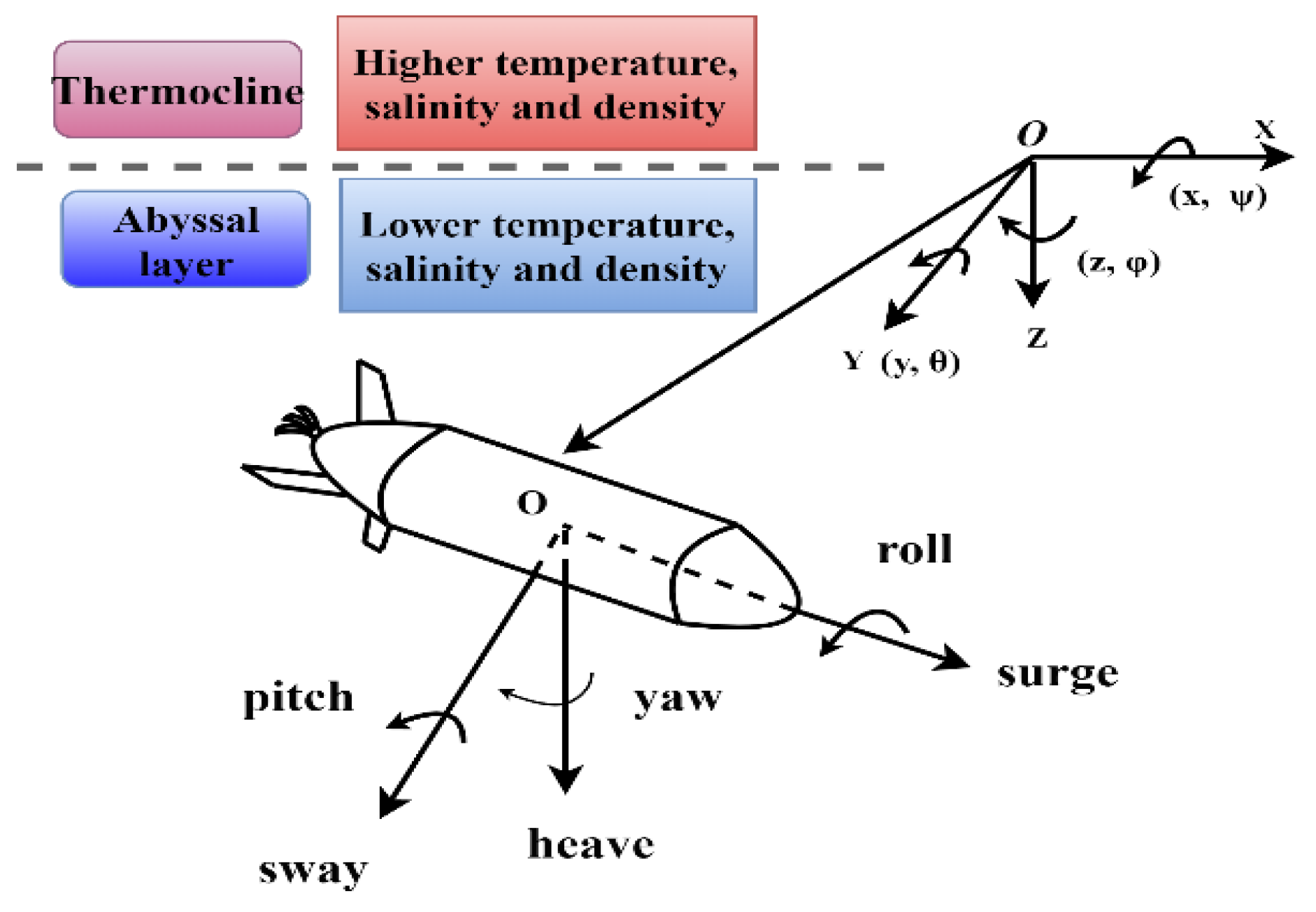
2.1. Problem Description

There are 18 kinds of factors that directly affect the drift motion of AUV, which are divided into 4 categories, including current, wind, and wave, as well as the size of the AUV. Among them, currents are divided into three types: density currents (m/s), wind currents (m/s), and tidal currents (m/s). Wind is divided into 4 types: wind direction (°), wind speed (km/s), crosswind direction (°), and crosswind speed (km/s). Waves include 4 types: action coefficient of wave drifting force, effective wave height (m), wavelength ($\mathsf{\mu }$m), and wave number (nm). In addition, there is target size (m³), temperature (°), salinity (‰), density (g/cm³), gravitational acceleration (m/s²), diving depth (m), and fluid resistance (N).

Under the combined influence of the torque and force generated by the many above factors, the AUV produces six degrees of freedom of space motion after it is out of control at the great diving depth. The six degrees of freedom are surge, sway, heave, roll, pitch, and yaw. The heave is floating upward under the action of residual buoyancy. During the floating process, the AUV passes through different ocean layers. According to the difference of influencing factors, it is mainly divided into deep ocean layer and thermocline, as shown in the following Figure 1.

During the floating process, the marine factors affecting drift motion are similar when the AUV is in the ocean deep layer and middle layer. However, there is a huge change of the composition of influencing factors when it drifts to the thermocline. The main reasons for the change are the appearance of the prevailing wind on the ocean surface and the sudden changes of ocean water temperature, salinity, and density with depth, as shown in Figure 2.

Figure 2a shows that in the thermocline at a depth of 200 m, the temperature of the ocean water rises rapidly. Similarly, Figure 2b,c also show that there is a sudden change in the ocean salinity and density values in the thermocline, which makes the density distribution of the thermocline uneven. Causing the ocean surface to tilt and seawater flow. Finally, a larger density flow and a change in fluid force are caused [19].

In addition, waves are formed by the wind on the surface of the ocean, and the friction of the wind on the ocean surface and the pressure exerted by the wind on the windward side of the waves force the ocean water to move forward to form wind-driven currents. However, the action range of waves and wind-driven currents can only extend to the thermocline. Based on the above analysis, a new AUV drift track prediction framework based on modified neural network is proposed to solve the problem of feature drift during AUV drift.

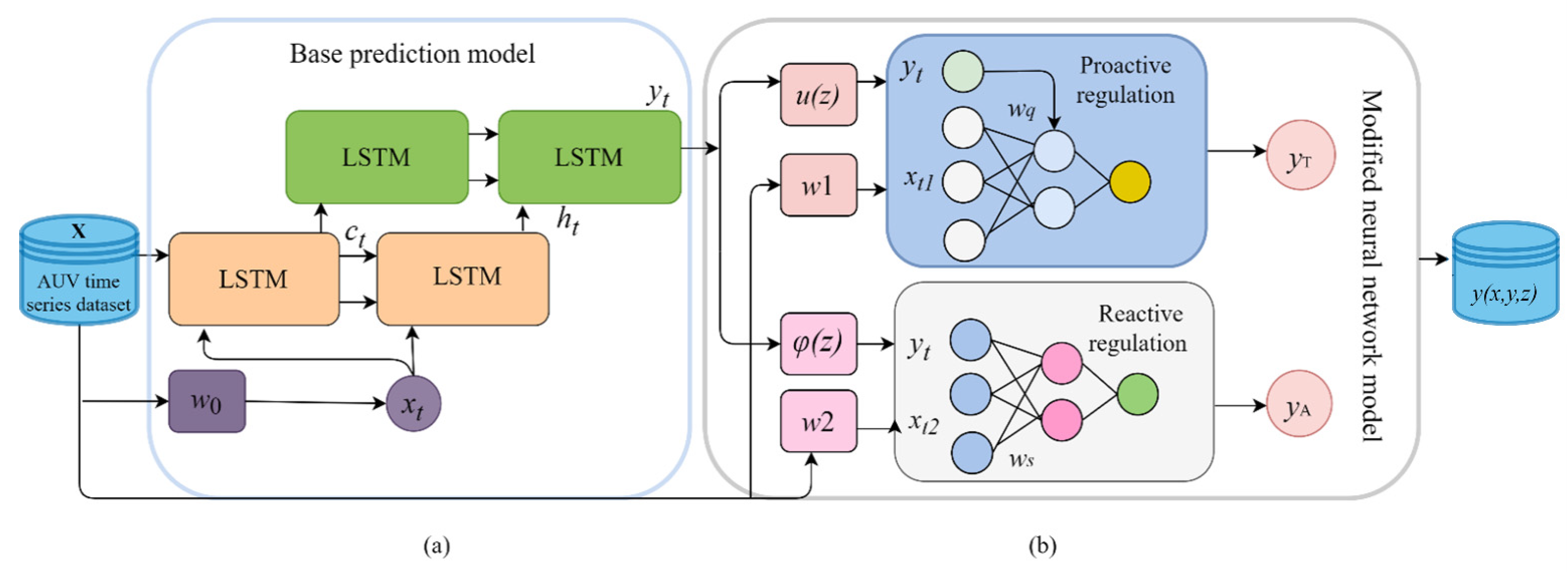
2.2. The Framework of AUV Drift Track Prediction

To help solve the problem of AUV drift in different ocean layers, an AUV drift track prediction framework based on a modified neural network is proposed. The framework consists of two different modules, as shown in Figure 3. As can be seen in Figure 3a, it is the base model predictor based on LSTM, which realizes the basic prediction of AUV drift track in real time and obtains the prediction result $y_t\left(x,y,z\right)$.

Long short-term memory (LSTM) [20] is a special RNN, which is mainly used to solve the problem of gradient disappearance and gradient explosion during long sequence training. Compared with RNN, which has only one transmission state $h_t$, LSTM has two transmission states, one cell state $C_t$ and one hidden state $h_t$. The internal structure of LSTM is to control the transmission state through the three gated states. Based on the $\sigma$ function, the extracted effective information is filtered, and each component is rated (0~1). The higher the rating, the more memories will enter the unit state. Therefore, LSTM can perform better in longer sequences than ordinary RNN. Figure 3b is a modified neural network model based on the emotion modulation mechanism proposed in this paper. The model includes two different modules, which are Proactive Modulation Module and Response Modulation Module. The correction track relies on the prediction results $y_t$ of the base prediction model. Since the depth of AUV prediction in the deep layer is only related to the residual buoyancy which is mainly related to density.

It can be seen in Figure 2c that the density of the deep ocean layer changes more slowly, so the base model is more accurate for depth prediction. Therefore, the ocean stratification of AUV is judged in real time by depth. According to the depth variation rule of thermocline in study [21], the depth of the thermocline in the sea area with the data obtained in this paper is 200 meters below sea level. By judging the $z$ variables in $y_t$, the different correction modules are entered. When$\left|z\right|\ge 200$, the prediction results of the base prediction model in the deep ocean layer is fine-tuned by the Proactive Modulation Module to obtain the prediction results $y_T$. When$\left|z\right|<200$, the Response Modulation module corrects the prediction results of the base model in real time when the marine environment changes greatly after the AUV drifts to the thermocline. The results $y_A$ are obtained by real-time corrections of the prediction results of the base model. The calculation method of the framework results is as Equations (1)–(3):

$$y_t=f\left(x_t·W+y_{t-1}·V+b\right)$$

(1)

$$y_T=f_T\left(\left(\lambda y_t·\mu \left(t\right)\right)w_q+x_{t1}·v_q\right)·w_T+\phi$$

(2)

$$y_A=f_A\left(\left(y_t,x_{t2}\right)·W_s+\varphi \right)$$

(3)

Since the AUV track prediction problem is dependent on the time dimension, so the base model of the AUV drift track prediction framework is selected as the LSTM model with higher prediction accuracy for short sequences [22]. The structure of the AUV track prediction model based on LSTM is shown in Figure 4.

The AUV time series data set is $X\left(x_0,x_1,x_2\cdots x_{17}\right)$. When AUV drifts in the deep ocean layer, the main influencing factor is $x_t$, which is expressed as in Equation (4):

$$\mathit{X}\left\{\begin{array}{ccc}{\mathit{x}}_{\mathit{t}}^{\left(\mathbf{0}\right)}& \cdots & {\mathit{x}}_{\mathit{t}\mathbf{+}\mathit{l}}^{\left(\mathbf{0}\right)}\\ \cdots & \cdots & \cdots \\ {\mathit{x}}_{\mathit{t}}^{\left(\mathbf{17}\right)}& \cdots & {\mathit{x}}_{\mathit{t}\mathbf{+}\mathit{l}}^{\left(\mathbf{17}\right)}\end{array}\right\})\stackrel{{\mathit{w}}_{\mathbf{1}}}{\to }\left\{\begin{array}{ccc}{\mathit{x}}_{\mathit{t}}^{\left(\mathbf{0}\right)}& \cdots & {\mathit{x}}_{\mathit{t}\mathbf{+}\mathit{l}}^{\left(\mathbf{0}\right)}\\ \cdots & \cdots & \cdots \\ {\mathit{x}}_{\mathit{t}}^{\left(\mathbf{8}\right)}& \cdots & {\mathit{x}}_{\mathit{t}\mathbf{+}\mathit{l}}^{\left(\mathbf{8}\right)}\end{array}\right\},$$

(4)

where $x_t$includes density current (m/s), tidal current (m/s), target size (m³), temperature (°), salinity (‰), density (g/cm³), gravitational acceleration (m/s²) [23], dive depth (m), and fluid resistance (N) [24]. The hidden layer adopts three layers of LSTM, and the hidden neurons of each layer are set to 128, 64, 32.

Besides, the Adam optimizer is used to realize the simple and efficient calculation of the model. Secondly, an L1 regularization term is added to the loss function to help ensure the predictive performance of the model on samples outside the training set. The formula is as Equation (5):

$$\begin{array}{c}J=J_0+L\\ J_0=\underset{\omega }{\min }{\displaystyle \sum _{i=1}^N}{\left({\omega }^T{x}_i-y_i\right)}^2,\\ L=\lambda \Vert \omega {\Vert }_2^2\end{array}$$

(5)

where $J_0$ represents the original loss function, and $L$ represents the penalty term added by regularization. $\omega$is the coefficient of the characteristic, and $\lambda$ represents the regularization coefficient which prevents over fitting by constraining the possible value space of $\omega$.

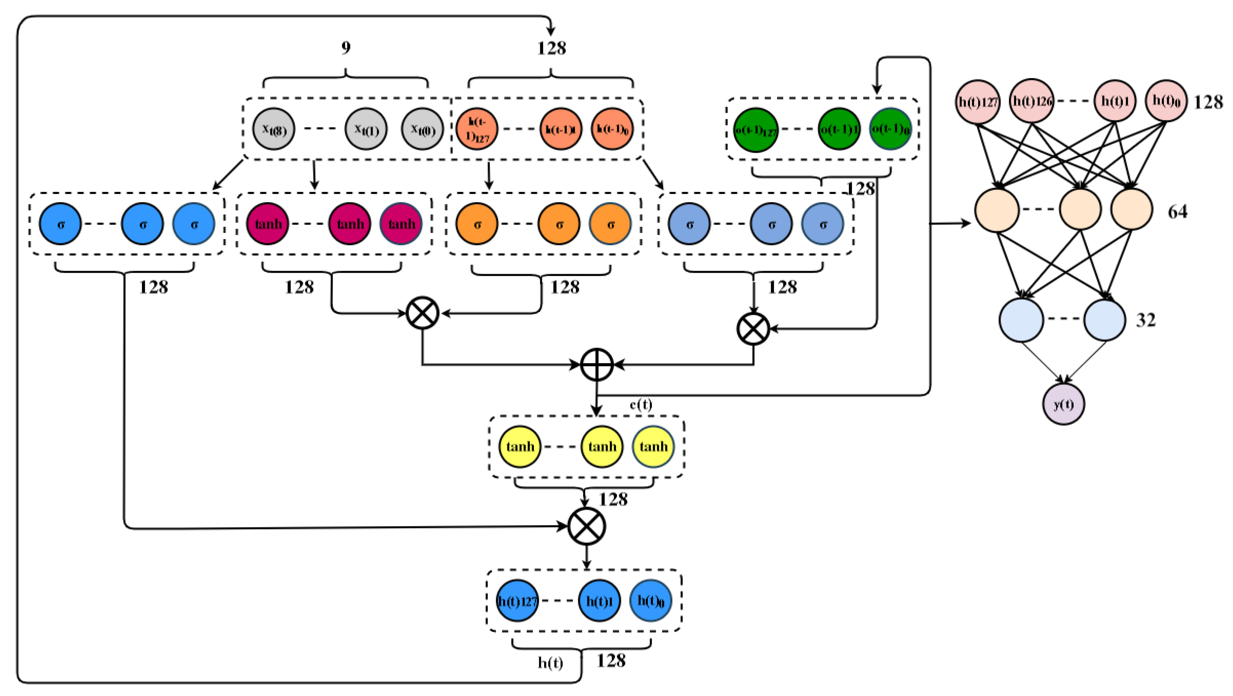
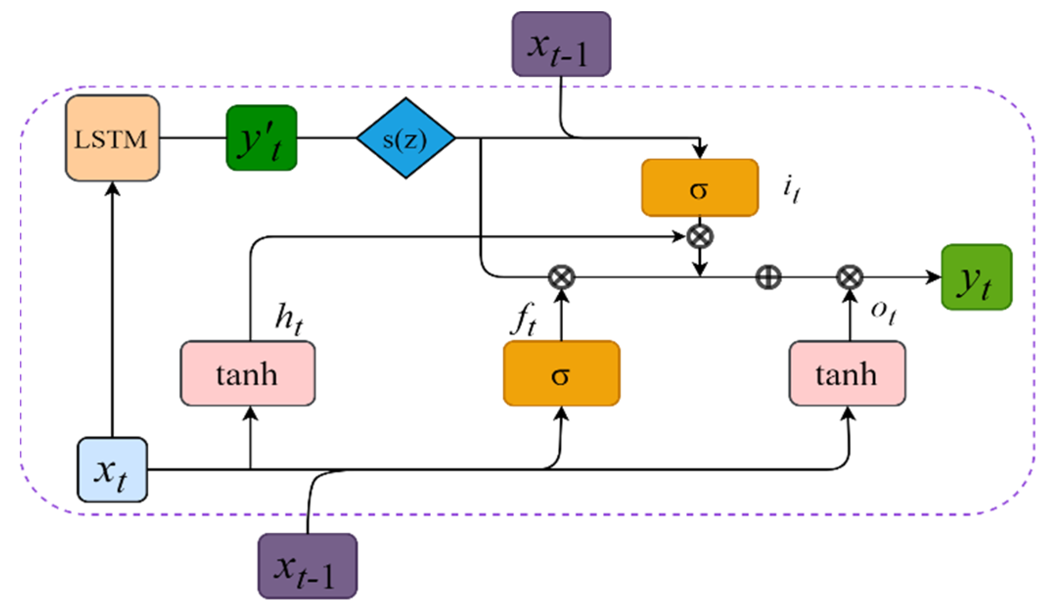
2.3. The Prediction Model of ECRNet

At present, due to the continuous development and progress of deep learning and machine learning methods, it also provides technical support for time series prediction, and has made great progress in accuracy and intelligence [25]. However, on account of the lack of understanding of professional knowledge in certain specific engineering application fields, problems of reduced accuracy and difficult model convergence will still occur when encountering complex problems unique to the application fields with full description of their characteristics and corresponding weight initialization. Therefore, this section proposes a modified neural network for the AUV drift track prediction problem. This network can correct and compensate for the prediction deviation caused by the insufficient understanding of the LSTM model of the marine environment in real time, and improve the accuracy and continuous learning of the neural network results.

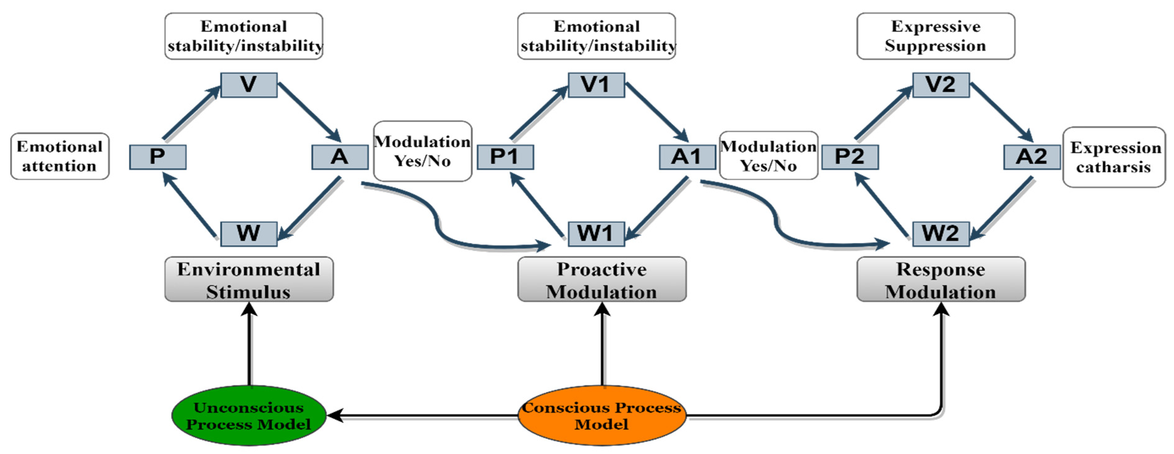
2.3.1. Emotion Modulation Mechanism

In the emotional modulation mechanism proposed by cognitive psychology [26], we are prone to emotional fluctuations when encountering changes in the surrounding scene or emergencies. Improper emotions will accumulate over time and eventually lead to deviation from normal emotions without timely adjustment correction. The human body can accumulate experience and exercise to learn a timely correction of improper emotional ability and the specific tuning process can be seen in Figure 5.

The emotional modulation mechanism of humans is divided into two modes: Proactive Modulation and Response Modulation [27]. The Proactive Modulation mode plays a role when the emotion fluctuation is within the controllable range of the brain perception: by analyzing the factors that stimulate emotions, and paying attention to the optimistic factors and restoring emotional balance by superimposing the happy factors on the negative emotions or ignoring the stimulating factors that cause emotions to rise to help restore emotional balance. Therefore, Proactive Modulation is through continuous learning and accumulation of different stimuli in the emotional value of the proportion of $P$, and the inappropriate emotional proportion of $W1$will be adjusted and corrected to the balanced emotional proportion of $V1$when encountering the same scene.

If improper emotions continue to accumulate or the external environment and scene show strong changes, the normal state of emotional fluctuations beyond the controllable range of the brain will deviate to a large extent from the normal emotional state. This means that the Response Modulation mode will be entered. It is necessary to vent the original emotions in some way and rebuild stable emotions through the current environmental factors. In addition, people can suppress the initial inappropriate emotion through the positive factors in the stimulus and adjust the emotion to a normal state.

Therefore, the first path of Response Modulation is the degree $\lambda$ and proportion $P2$ of learning to suppress or vent improper emotions. The second path is the proportion $V2$ of positive factors in the change of learning environment. The combination of the two paths will adjust and correct emotions to a new stable state $A2$.

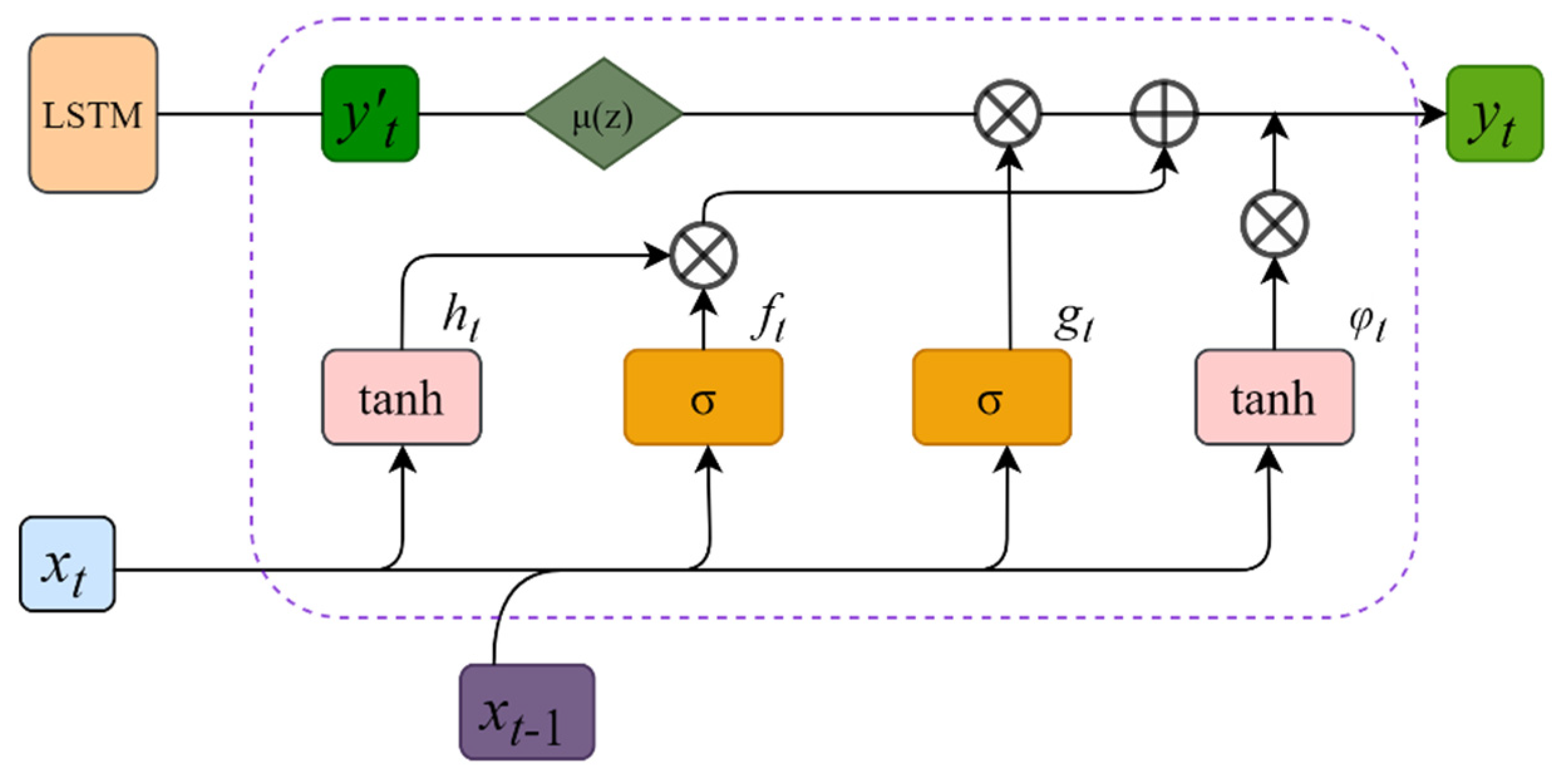
2.3.2. Modified Neural Network

The modified neural network aims to establish a short-term dynamic model to compensate and adjust the prediction bias accumulation in the long-term mode of the prediction model. Inspired by the emotion modulation mechanism, the prediction bias of the LSTM model in different ocean layers is modified by two correction strategies.

• Proactive Modulation Module

The structure of the Proactive Modulation module is shown in Figure 6. The input of it consists of two parts which includes the prediction result $y{\prime }_t$ of the base prediction model and the $x_t$ obtained by matrix selection of the features in the feature factor data set$X_t$.

The Proactive Modulation module is mainly composed of two evaluation functions and output functions, and its specific workflow is as follows. The first step of it is that the $z$ variable in the input $y{\prime }_t$ is judged by the $\mu \left(z\right)$ function to decide whether to enter the module for correction. The formula of $\mu \left(z\right)$ is as Equation (6):

$$\mu \left(z\right)=\left\{\begin{array}{cc}1 ,& z<-200\\ 0 , & z\ge -200 \end{array}\right.,$$

(6)

where $z$represents the depth of the AUV drift predicted by the base model. It can be seen from Equation (6) that the value of $\mu \left(z\right)$is 1 when $z<-200$, and then the Proactive Modulation module is activated. The input $x_t$ is processed through the full connection layer with tanh as the activation function to obtain the position state information $h_t$ at the current time. The formula is as Equation (7):

$$h_t=\tan \mathrm{h}\left(W_h·x_t+b_h\right)$$

(7)

The next step is to process and evaluate the two parts of location information $h_t$ and$y{\prime }_t$ through two evaluation functions. This step is divided into two parts. The first part operation is handled by an evaluation emphasis function $e_t$ to obtain emphasis information $E_t$. Based on the function, by examining and comparing the information between $x_t$ and $x_{t-1}$ to output a value of 0–1. The closer the value is to 1, the higher the degree of emphasis is. The closer the value is to 0, the information will be ignored. The formula is as Equation (8):

$$\begin{array}{c}{e}_t=\sigma \left(W_e·[x_t,x_{t-1}\right]+b_e),\\ E_t=e_t\ast h_t\end{array}$$

(8)

The next operation is handled by an evaluation neglect function $g_t$ to decide what information to ignore to obtain the final information $N_t$. The formula is as Equation (9):

$$\begin{array}{c}{g}_t=\sigma \left(W_g·[x_t,x_{t-1}\right]+b_g),\\ N_t=g_t\ast y{\prime }_t\end{array}$$

(9)

The last step is that the modified prediction result $y_t$ is obtained through the selectivity of the output function to the information modified by the rating function. The formula is as Equation (10):

$$\begin{array}{c}{y}_t={\phi }_t ·\tan \mathrm{h}\left(O_t\right)\\ {\phi }_t=\tan \mathrm{h}\left(W_{\phi }·[x_t,x_{t-1}\right])\\ O_t=N_t+E_t\end{array}$$

(10)

To help the model learn more accurately and quickly, the value score of each feature is calculated and normalized based on the principle of permutation feature importance [28]. The value score of each feature is used as the initialization parameter of the AUV drift track prediction model to help the model converge quickly and save the training prediction time to get the global optimal solution.

Firstly, based on the trained base prediction model, random shuffle is performed for one feature column at a time. Then, input the model for prediction, and record each feature column of change and its corresponding Loss. Each Loss is the corresponding feature importance. The greater the Loss, the more important the feature is to the model. The formula for calculating the feature value score is as Equations (11) and (12):

$$s=\frac{1}{m}{{\displaystyle \sum }}_{i=1,j=1,2,\cdots 9}^{m}L\left(x_t,x_k\right)$$

(11)

$$L\left(x_t,x_k\right)=\frac{1}{2}{\left|y-f\left(x_t\right)\right|}^2$$

(12)

$s$ represents the value score of each feature, and$L\left(x_t,x_k\right)$represents the loss value predicted by the random shuffle model for the feature k. The value score of each feature obtained by calculation is shown in Figure 7:

Through the normalization formula, the value score of each feature is mapped to the range of (0,1) to initialize the parameters of the Proactive Modulation module. The normalization formula is as Equation (13):

$$s^{\prime }=\frac{s_i-\min \left(s_i\right)}{\max \left(s_i\right)-\min \left(s_i\right)}$$

(13)

2.

Response Modulation Module

The input of the Response Modulation Module’s different part from the Proactive Modulation Module is the $x_{t }$obtained from the feature selection in the feature factor data set $X_{t }$, and then one decides whether to enter the response modulation module by activating the function $s\left(z\right)$. The formula of$s\left(z\right)$is as Equation (14):

$$s\left(z\right)=\left\{\begin{array}{ll}0,& z<-200\\ 1 , & z\ge -200\end{array}\right.$$

(14)

It can be seen from Figure 8 that the Response Modulation module is mainly composed of the reward function and suppression function. The first step of it is the same as the Proactive Modulation module to obtain the position state information $h_t$ at the current time as Equation (7). The next step is to process and evaluate location information $h_t$ and$y{\prime }_t$ by two steps. The first operation is handled by a reward function $i_t$ to obtain compensating information $I_t$. The formula is as Equation (15):

$$\begin{array}{c}{I}_t=x_t\ast i_t\\ i_t=\sigma \left(W_i·\left[x_t,x_{t-1}\right]+b_i\right), \end{array}$$

(15)

$i_t$ is a number between 0 and 1. The closer it is to 1, the greater the degree of reward for $x$, and the more information retains from $h_t$. The next operation is handled by the suppression function $f_t$ to obtain the information $F_t$. The formula is as Equation (16):

$$\begin{array}{c}{F}_t=x_t\ast f_t\\ f_t=\sigma \left(W_f·\left[x_t,x_{t-1}\right]+b_f\right), \end{array}$$

(16)

The $f_t$ also is the value between 0 and 1. The closer it is to 1, the more information in $y{\prime }_t$is suppressed and ignored and the less information is learned and retained by the network. Finally, the updated information $I_t$ and $F_t$ is selected through the output function $o_t$ to obtain the final modified prediction result.

Figure 8. Structure of the Response Modulation module.

Figure 8. Structure of the Response Modulation module.

This section introduces the framework and prediction process of AUV drift track prediction based on a modified neural network. The structure and prediction principle of each module of the modified neural network is introduced in detail. Then, in the next section, we will verify the improvement of the accuracy of the prediction results based on our mothed through experiments.

3. Experiments and Results

This section compares and analyzes the time series prediction models in the field of deep learning to test whether the modified neural network improves the prediction accuracy. The time series prediction models include LSTNet [29], Transformer [30], RNN [31], LightGBM [32], and base prediction models based on LSTM.

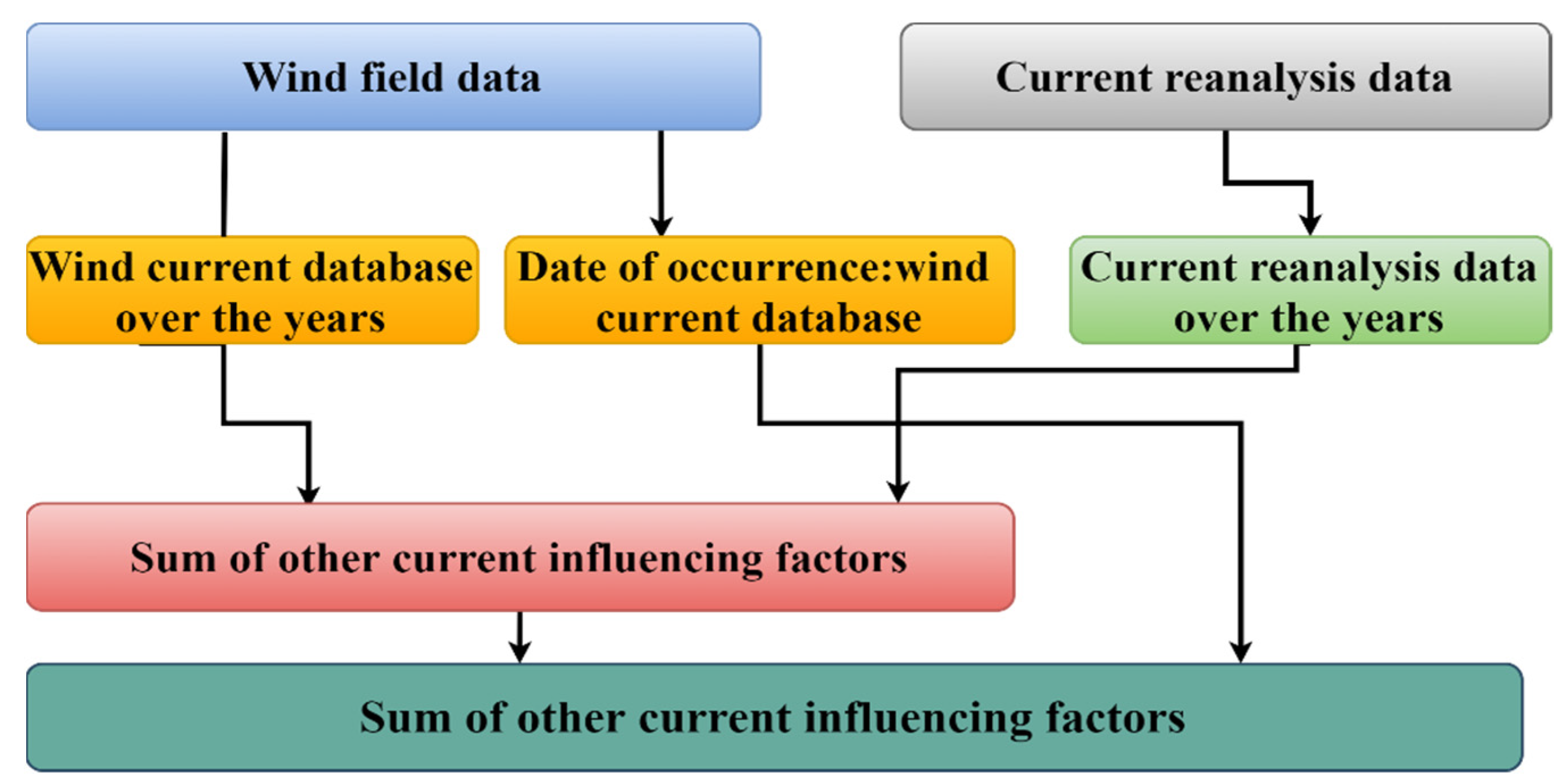
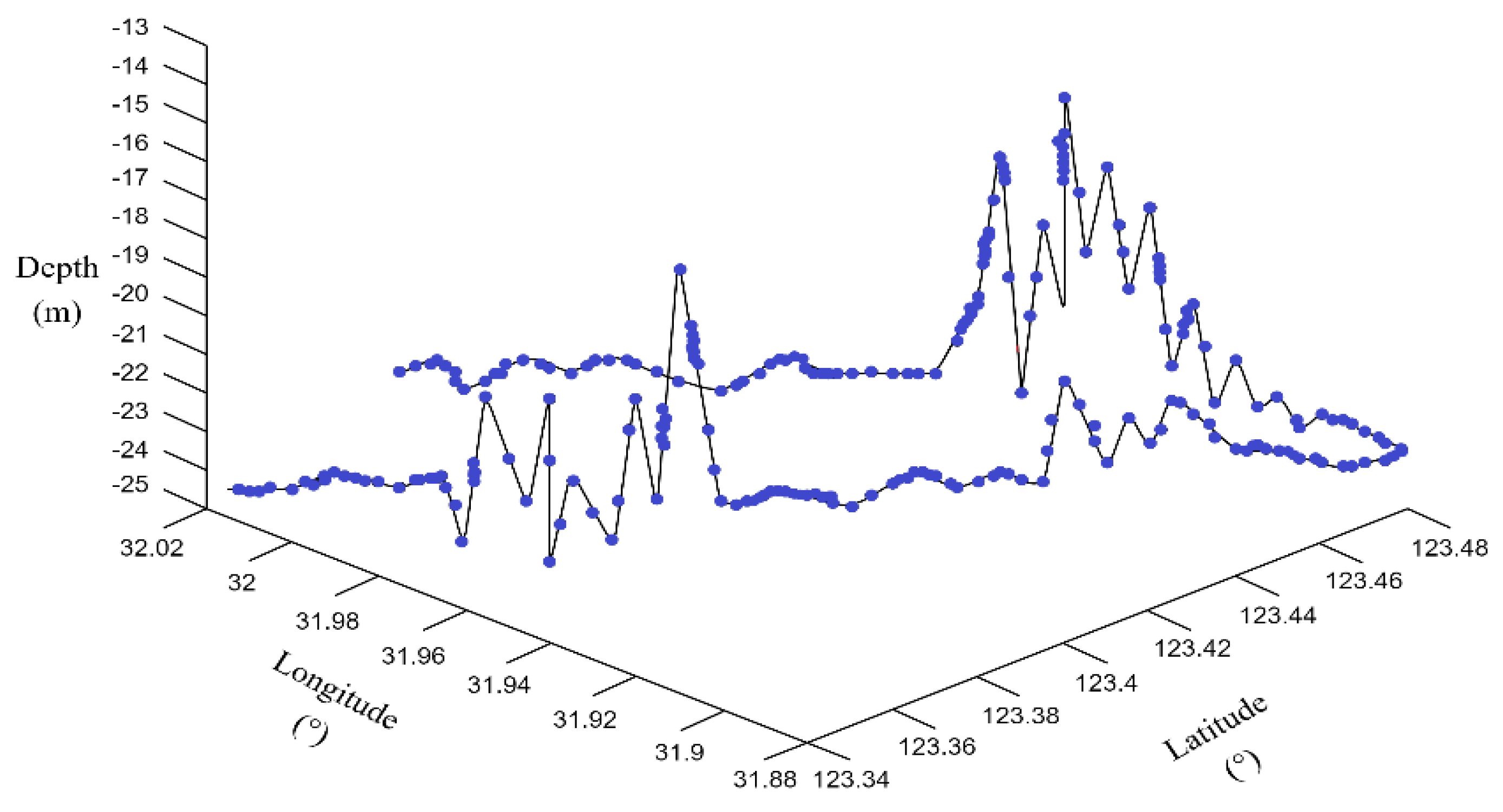
3.1. Data Processing

The experimental model prediction uses the real drift position data returned by the Ultrashort Baseline (USBL) positioning system and sensor mounted on the AUV and the real-time meteorological data obtained by the National Marine Data Science Center [33] and the National Meteorological Science Data Center [34]. However, some ocean factors such as waves and currents that affect the AUV drift track cannot be directly obtained by the observed data. There is a need to establish a complete data set based on the reanalysis data of current and wave from satellite data [35,36,37]. The process of establishing the current database is shown in Figure 9.

Firstly, the wind current database near the date of the event is constructed to obtain the reanalysis data from near the date of the event [38]. The fixed current data are compared with the analysis data of the current over the years, and the difference is taken as the sum of other current influencing factors near the date. Then, the synthesis of other ocean-current influencing factors is added to the wind current database constructed near the date of the incident, and that is the real ocean current database of the surface layer on the date of the incident. The calculation of wind current is based on the empirical formula obtained by the Polish Maritime University [39] as Equation (17):

$$V_{wc}={\left(0.230446+0.0070957V_w\right)}^2\pm 0.17$$

(17)

The value range of the wind current is obtained through wind speed $V_w$ and the maximum value is taken as the value of the wind current. The direction of the wind current is obtained from the following equation, to obtain the direction$c$ of the wind current as Equation (18):

$$c=-35.338+3587.78/V_w$$

(18)

In the data set of this paper, the drift time of the crashed AUV is from 13:00 on 3 November 2019 to 18:00 on 8 November 2019, and the data collection site is the Wolfberry scene spot. The maximum depth of the AUV diving is 800 m, the real-time wind speed is 11 m/s, and the wind direction is northwest wind. The actual AUV drift track is shown in Figure 10.

We use the four indicators shown in the following formula to evaluate the prediction accuracy of our proposed prediction model.

• Mean square error (MSE) describes the mean square error between the predicted and actual values in three dimensions:

$$\mathrm{MSE}=\sqrt{\frac{{{\displaystyle \sum }}_{k=1}^n{\left(y_k-\widehat{y_k}\right)}^2}{N}}$$

(19)

$$y_k=\sqrt{{\left(l_1-l_2\right)}^2+{\left({\phi }_1-{\phi }_2\right)}^2+{\left(d_1-d_2\right)}^2}$$

(20)

• Root means square error (RMSE) is the square root of the difference between the predicted value and the actual value in three dimensions:

$$\mathrm{RMSE}=\sqrt{\mathrm{MSE}}$$

(21)

• Mean absolute error (MAE) is the average of the absolute differences between the predicted and actual values.

$$\mathrm{MAE}=\frac{1}{m}{\displaystyle \sum }_{i=1}^m\left|y_k-\widehat{y_k}\right|$$

(22)

• Relative error (RE) reflects the deviation of the measured value from the true value and can better reflect the credibility of the measurement:

$$\mathrm{RE}=\frac{\widehat{y_k }-y_k}{ y_k}·100\%$$

(23)

where $N$is the number of predicted data,$y_k$is the measured AUV drift track, $\widehat{y_k }$ is the predicted drift track,$l$ is the longitude of the track,$\phi$ is the latitude of the track, and$d$is the depth of the track.

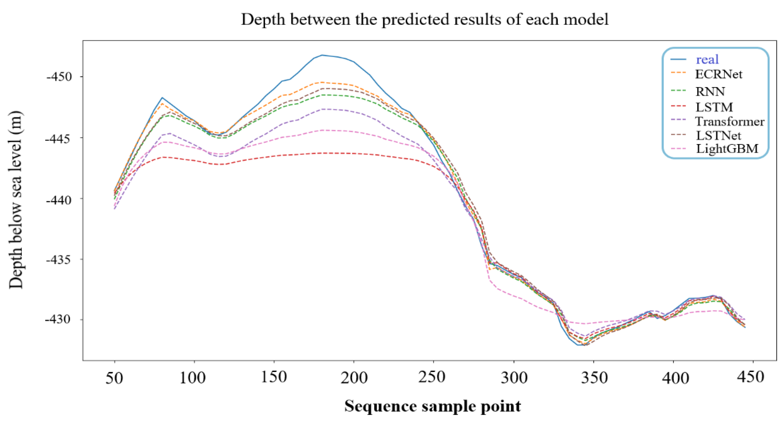
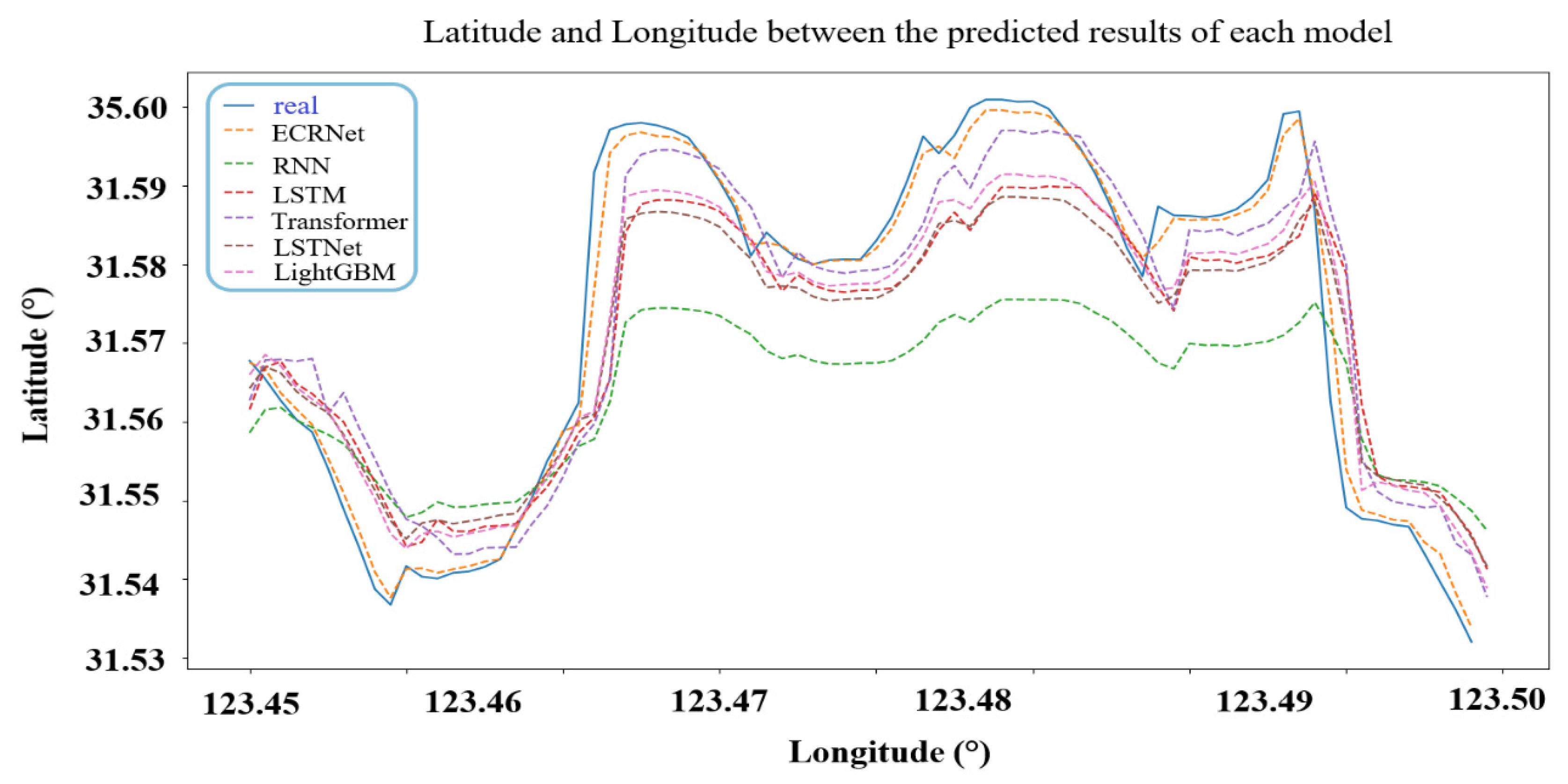
3.2. Experimental Analysis

In this experiment, the results of different prediction models in the deep ocean layer and the thermocline were compared and analyzed. In addition to the uncorrected LSTM-based prediction model in our framework, the other time series prediction models with better prediction effect in deep learning fields are also selected, which are LSTNet, Transformer, RNN, and LightGBM. Each of the above models uses the same training set and test set. In this experiment, the test set is the track sequence dataset of the deep ocean layer, and the experimental comparison is carried out under the same conditions.

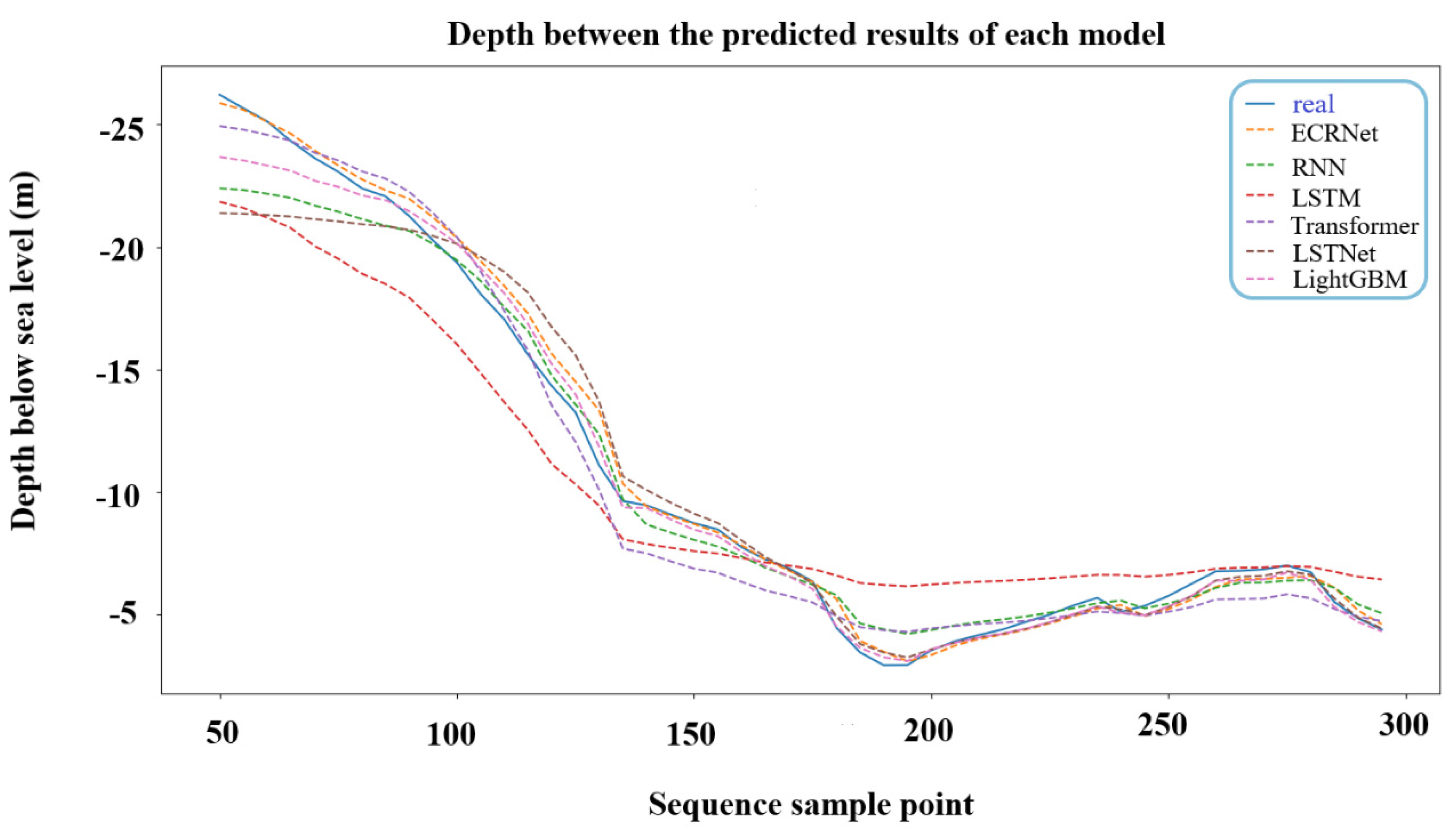
• Prediction results of drift track of models in the deep ocean layer

In the deep ocean layer, 500 track sequences are randomly selected as the test set. Regarding the comparison between the prediction results obtained by each model on the test set and the real track sequence of latitude, longitude, and depth, the result is shown in Figure 11 and Figure 12.

Figure 11 shows the AUV drift track prediction results of Latitude and Longitude based on ECRNet, RNN, LSTM, LSTNet, Transformer, and LightGBM, respectively.$real$ represents the real drift track sequence, and the ECRNet represents the predict result by us. It can be seen that the sequence of $real$ and ECRNet has the best fitting effect in Figure 11. Figure 12 shows the track prediction results for depth. It still shows that among the six models shown in Figure 12, the prediction results of our model for depth are the closest to the actual results. Therefore, this paper proposes a prediction method which more accurately fits the predicted results with the real drift track sequence.

Table 1. Prediction performance of different models in deep ocean layer.

Model Type	Relative Error (%)	MSE (10−3)	RMSE (10−3)	MAE (10−3)
ECRNet (Our Method)	0.0251	2.167	1.472	1.369
RNN	0.1643	9.418	3.069	2.923
LSTM	0.1026	5.651	2.377	2.164
Transformer	0.0863	4.002	2.013	1.981
LSTNet	0.0635	2.042	2.836	2.653
LightGBM	0.0914	4.822	2.196	2.032

shows the predictive performance of the above six models.

It can be seen from Table 1 that when drifting in the deep ocean layer, the base prediction model based on LSTM is first used for prediction. Owing that $z<-200$, the Proactive Modulation Module of the modified neural network is used for correction. Compared with the results of other time series prediction models, the modified prediction results have achieved better performance (MSE = 2.167, RMSE = 1.472, MAE = 1.369), where the three indicators have been greatly improved. Besides, the three indicators are 3.484, 0.905, and 1.795 lower than the predicted results of the unmodified basic model, respectively. In addition, in order to show the advantages of our model more directly, we also express the prediction performance of each model through the relative error index. The minimum relative error of our model is 0.0251%. Therefore, the modified neural network in this paper has greatly improved the prediction accuracy of the prediction model in the deep ocean layer, and better fitted the AUV drift track.

2.

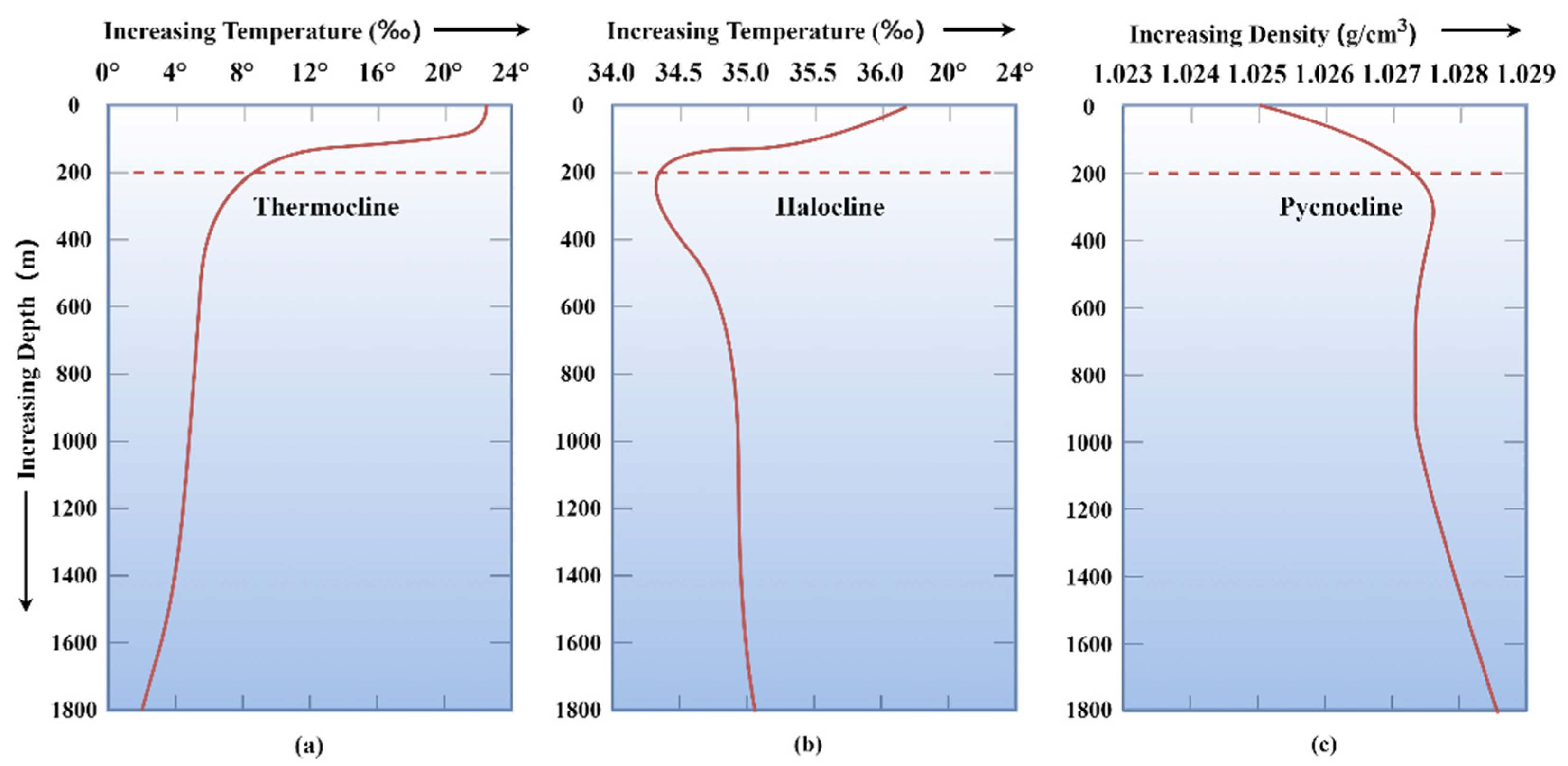
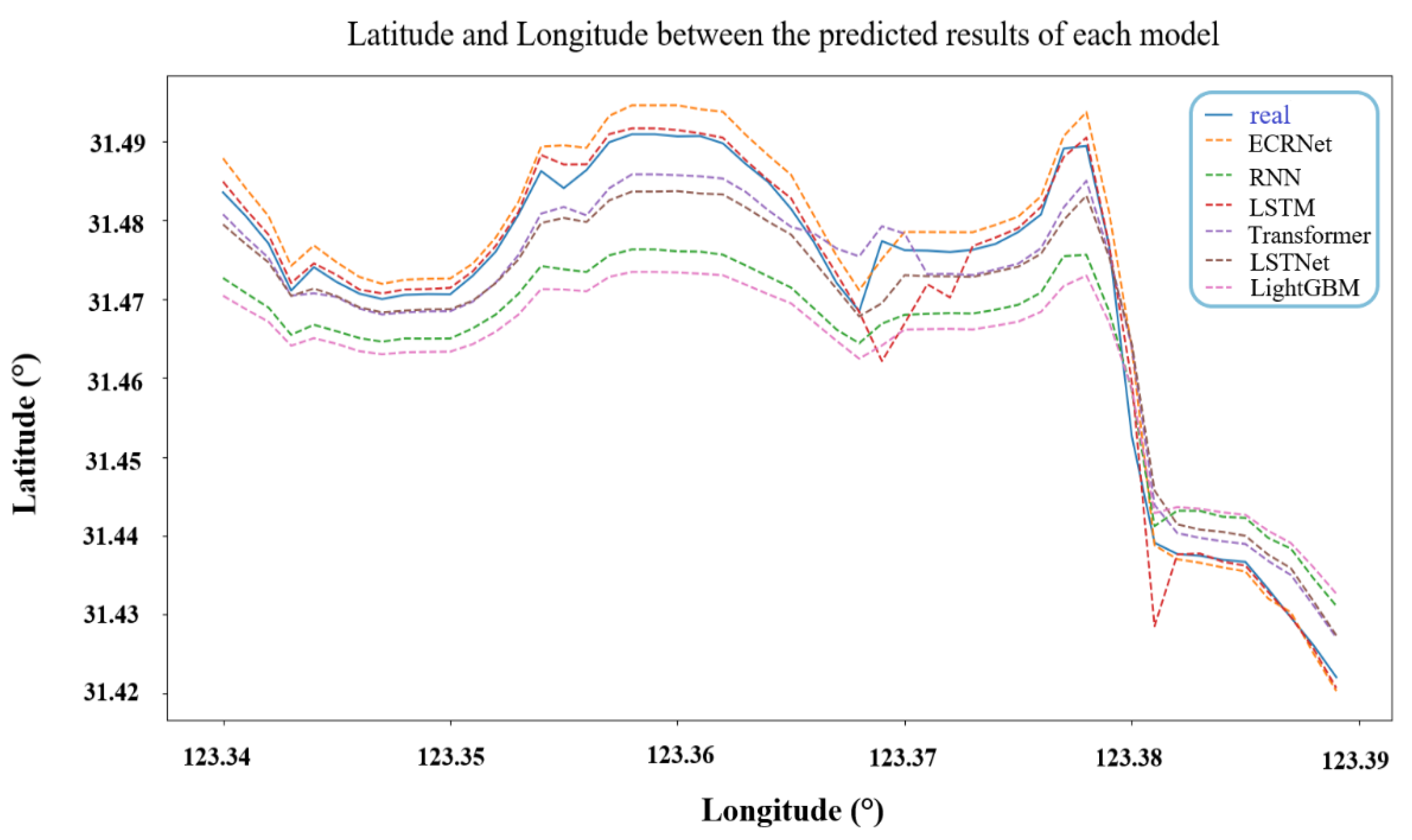
Prediction results of drift track of models in the thermocline

The prediction results of each model on the test set of the thermocline were compared with the real track sequence, the results of the Latitude and Longitude are shown in Figure 13, and the results of depth are shown in Figure 14. Owing that $z\ge -200$, the results of the base prediction model were modified by the Response Modulation module. Figure 13 shows that $real$and ECRNet achieve the best fitting effect again based on our model. Besides, Figure 14 also shows that the track prediction result of depth based on the ECRNet obtains the best fitting effect. The above results prove that the Response Modulation module implements the feature drift problem for different ocean layers and ensures more accurate and continuous prediction of the AUV drift track.

Table 2. Prediction performance of different models in the thermocline.

Model Type	Relative Error (%)	MSE (10−3)	RMSE (10−3)	MAE (10−3)
ECRNet (Our Method)	0.0667	3.319	1.822	1.723
RNN	0.328	27.762	5.269	5.126
LSTM	0.236	16.991	4.128	4.096
Transformer	0.125	12.341	3.513	3.422
LightGBM	0.269	19.148	4.625	4.103
LSTNet	0.253	17.118	4.125	4.093

shows the prediction performance of the above six models when the feature drift problem occurs after the AUV enters the thermocline. In Table 2, the prediction results corrected by the Response Modulation Module have a greater improvement in prediction performance than other models.

Compared with the results before correction, the three evaluation indicators were improved by 13.672, 3.306, and 2.373, respectively. Besides, the ECRNet obtains the better relative error, which is 0.0667%. Therefore, the influence of feature drift on the prediction accuracy is greatly alleviated, and the prediction performance of the model is still guaranteed after entering the thermocline with more accurate prediction results.

4. Discussion

In this paper, in order to solve the problem of feature drift when AUV drifts in different ocean layers after the AUV crash, a new method of AUV drift track prediction based on a modified neural network is proposed.

• The modified neural network establishes two different correction modules of Proactive Modulation and Response Modulation by imitating two strategies of people to regulate emotional fluctuations. The prediction errors caused by feature drift when the AUV drifts to the deep ocean layer and thermocline are corrected respectively.
• The modified neural network realizes the continuity of prediction results and the ability of sustainable learning of the model to a certain extent through different activation functions, selection weights, and different modified strategies.
• The modified neural network reduces computation in the time dimension, and the model structure is simpler for more accurate and faster training and prediction.

5. Conclusions

To help solve the difficulty of feature drift in the process of AUV drift, a new method of AUV drift track prediction based on a modified neural network is proposed. The modified neural network realizes error correction in the deep ocean layer and the thermocline through two different modules of Proactive Modulation and Response Modulation. The experimental results show that the proposed method has better prediction performance than other time series prediction models in two ocean layers. MSE, RMSE, and MAE all have good improvement. In the deep ocean layer, the three error indexes are reduced by 3.484, 0.905, and 1.795, respectively, compared with the uncorrected prediction model, and it is reduced by 13.672, 3.306, and 2.373, respectively, in the thermocline.

The prediction model proposed in this paper has achieved good prediction accuracy in the AUV track prediction of the crash. Nonetheless, this dataset is only in one ocean area. As a matter of fact, the AUV performs tasks in different and unknown ocean areas, and the data distribution of the influencing factors in the unknown ocean area changes greatly. How to improve the correction ability of the correction network and improve its generalization ability will be the focus of future research.

References

1. Tanakitkorn, K.; Wilson, P.A.; Turnock, S.R.; Phillips, A.B. Depth control for an over-actuated, hover-capable autonomous underwater vehicle with experimental verification. Mechatronics 2017, 41, 67–81. [Google Scholar] [CrossRef]
2. Corradini, M.L.; Orlando, G. A robust observer-based fault tolerant control scheme for underwater vehicles. J. Dyn. Syst. Meas. Control 2014, 136, 034504. [Google Scholar] [CrossRef]
3. Zhang, X.; Zhu, Y.; Zhang, J. An Algorithm for ocean Ice Drift Retrieval Based on Trend of Ice Drift Constraints from Sentinel-1 SAR Data. J. Coast. Res. 2020, 102, 113–126. [Google Scholar] [CrossRef]
4. Liu, X.; Zhang, M.; Rogers, E.; Wang, Y.; Yao, F. Terminal sliding mode-based tracking control with error transformation for underwater vehicles. Int. J. Robust Nonlinear Control 2021, 31, 7186–7206. [Google Scholar] [CrossRef]
5. Gao, Z.; Guo, G. Fixed-time sliding mode formation control of AUVs based on a disturbance observer. IEEE/CAA J. Autom. Sin. 2020, 7, 539–545. [Google Scholar] [CrossRef]
6. Michael, K.B. Real-Time Modeling of Cross-Body Flow for Torpedo Tube Recovery of the Phoenix Autonomous Underwater Vehicle (auv); Naval Postgraduate School: Monterey, CA, USA, 1998. [Google Scholar]
7. Gabl, R.; Davey, T.; Cao, Y.; Li, B.; Walker, K.L.; Giorgio-Serchi, F.; Aracri, S.; Kiprakis, A.; Stokes, A.; Ingram, D. Experimental force data of a restrained ROV under waves and current. Data 2020, 5, 57. [Google Scholar] [CrossRef]
8. Gabl, R.; Davey, T.; Cao, Y.; Li, Q.; Li, B.; Walker, K.L.; Giorgio-Serchi, F.; Aracri, S.; Kiprakis, A.; Stokes, A.; et al. Hydrodynamic loads on a restrained ROV under waves and current. Ocean. Eng. 2021, 234, 109279. [Google Scholar] [CrossRef]
9. Klamo, J.T.; Yeager, K.I.; Cool, C.Y.; Turner, T.M.; Kwon, Y.W. The Effects of Cross-Sectional Geometry on Wave-Induced Loads for Underwater Vehicles. IEEE J. Ocean. Eng. 2020, 46, 765–784. [Google Scholar] [CrossRef]
10. Zhang, Y.; Wang, L. Real-Time Disturbances Estimating and Compensating of Nonlinear Dynamic Model for Underwater Vehicles. Math. Probl. Eng. 2018, 2018, 5760841. [Google Scholar] [CrossRef]
11. Walker, K.L.; Gabl, R.; Aracri, S.; Cao, Y.; Stokes, A.A.; Kiprakis, A.; Giorgio-Serchi, F. Experimental Validation of Wave Induced Disturbances for Predictive Station Keeping of a Remotely Operated Vehicle. IEEE Robot. Autom. Lett. 2021, 6, 5421–5428. [Google Scholar] [CrossRef]
12. Guerrero, J.; Torres, J.; Creuze, V.; Chemori, A. Adaptive disturbance observer for trajectory tracking control of underwater vehicles. Ocean. Eng. 2020, 200, 107080. [Google Scholar] [CrossRef]
13. Chen, H.; Zhao, H.; Wang, N.; Guo, C.; Lu, T. Accurate track control of unmanned underwater vehicle under complex disturbances. China Ship Res. 2022, 17, 11. [Google Scholar]
14. Li, J.; Ming, K.; Farouk, N.; Xing-hua, C. Horizontal Plane Motion Control of AUV Based on Active Disturbance Rejection Controller. In Proceedings of the 27th Chinese Control and Decision Conference (CCDC), Qingdao, China, 6 November 2015. [Google Scholar]
15. Cao, X.; Wei, Y.; Heng, H.; Shen, Z. Dynamic surface backstepping trajectory tracking control of unmanned underwater vehicles with ocean current disturbances. Syst. Eng. Electron. Technol. 2021, 43, 1664–1672. [Google Scholar]
16. Hu, Y.; Liu, P.; Liu, Y. Ocean Stratification during the “Silent One Billion Years” Period. In Proceedings of the 34th Annual Meeting of the Chinese Meteorological Society (CCMS), Zhengzhou, China, 26–30 September 2017. [Google Scholar]
17. Peng, H. The Thermocline Changes in the South China Ocean and Its Response to ENSO. Master’s Thesis, Xiamen University, Xiamen, China, 2017. [Google Scholar]
18. Jiang, Y.; Li, Y.; Wang, Y.; Cao, J.; Li, Y.; Sun, Y.; Yin, Y.; Zhang, S. Gravity and buoyancy calculation of deep underwater robot in the whole ocean. J. Harbin Eng. Univ. 2020, 41, 6. [Google Scholar]
19. Huthnance, J.M.; Inall, M.E.; Fraser, N.J. Oceanic Density/Pressure Gradients and Slope Currents. J. Phys. Oceanogr. 2020, 50, 1643–1654. [Google Scholar] [CrossRef]
20. Hochreiter, S.; Schmidhuber, J. Long short-term memory. Neural Comput. 1997, 9, 1735–1780. [Google Scholar] [CrossRef]
21. Zhao, B. Basic characteristics and formation mechanism of strong thermocline in the Bohai Sea, Yellow Sea and northern East China Sea. J. Oceanogr. 1989, 11, 10. [Google Scholar]
22. Ghanbari, R.; Borna, K. Multivariate Time-Series Prediction Using LSTM Neural Networks. In Proceedings of the 2021 26th International Computer Conference, Computer Society of Iran (CSICC), Tehran, Iran, 3–4 March 2021. [Google Scholar]
23. Liu, X. Preliminary Study on the Variation Law of Gravity Acceleration around the Earth. New Course 2017, 12, 120. [Google Scholar]
24. Ji, W. Hydrodynamic study of sea surface drag coefficient. Ocean. Technol. 2002, 21, 4. [Google Scholar]
25. Li, W.; Deng, S.; Duan, Y.; Du, S. Time Series Forecasting and Deep Learning: Literature Review and Application Examples. Comput. Appl. Softw. 2020, 37, 62–70. [Google Scholar]
26. Zhu, C.; Jiang, Y.; Wang, Y.; Liu, D.; Luo, W. Arithmetic performance is modulated by cognitive reappraisal and expression suppression: Evidence from behavioral and ERP findings. Neuropsychologia 2021, 162, 108060. [Google Scholar] [CrossRef] [PubMed]
27. Berboth, S.; Morawetz, C. Amygdala-prefrontal connectivity during emotion Modulation: A meta-analysis of psychophysiological interactions. Neuropsychologia 2021, 153, 107767. [Google Scholar] [CrossRef] [PubMed]
28. Altmann, A.; Toloşi, L.; Sander, O.; Lengauer, T. Permutation importance: A corrected feature importance measure. Bioinformatics 2010, 26, 1340–1347. [Google Scholar] [CrossRef] [PubMed]
29. Lai, G.; Chang, W.C.; Yang, Y.; Liu, H. Modeling Long- and Short-Term Temporal Patterns with Deep Neural Networks. In Proceedings of the 41st International ACM SIGIR Conference on Research & Development in Information Retrieval, Ann Arbor, MI, USA, 18 April 2018. [Google Scholar]
30. Vaswani, A.; Shazeer, N.; Parmar, N.; Uszkoreit, J.; Jones, L.; Gomez, A.N.; Kaiser, Ł.; Polosukhin, I. Attention Is All You Need. In Proceedings of the 31st International Conference on Neural Information Processing Systems, Long Beach, CA, USA, 12 June 2017. [Google Scholar]
31. Wang, J.; Li, X.; Li, J.; Sun, Q. NGCU: A New RNN Model for Time-Series Data Prediction. Big Data Res. 2022, 27, 100296. [Google Scholar] [CrossRef]
32. Ke, G.; Meng, Q.; Finley, T.; Wang, T.; Chen, W.; Ma, W.; Ye, Q.; Liu, T. LightGBM: A Highly Efficient Gradient Boosting Decision Tree. Neural Inf. Process. Syst. 2017, 30, 3149–3157. [Google Scholar]
33. National Marine Data Center. Available online: http://mds.nmdis.org.cn/ (accessed on 5 June 2021).
34. National Meteorological Science Data Center. Available online: https://data.cma.cn/ (accessed on 5 June 2021).
35. Taqi, A.M.; Al-Subhi, A.M.; Alsaafani, M.A.; Abdulla, C.P. Estimation of geostrophic current in the Red Sea based on sea level anomalies derived from extended satellite altimetry data. Ocean. Sci. 2019, 15, 477–488. [Google Scholar] [CrossRef]
36. Xu, T.; Cao, Y. Numerical simulation of oceansonal variation of ocean circulation in the South China ocean. Coast. Eng. 2017, 36, 62–71. [Google Scholar]
37. Gómez-Orellana, A.M.; Fernández, J.C.; Dorado-Moreno, M.; Gutiérrez, P.A.; Hervás-Martínez, C. Building Suitable Datasets for Soft Computing and Machine Learning Techniques from Meteorological Data Integration: A Case Study for Predicting Significant Wave Height and Energy Flux. Energies 2021, 14, 468. [Google Scholar] [CrossRef]
38. Izaguirre, C.; Méndez, F.J.; Menéndez, M.; Losada, I.J. Global extreme wave height variability based on satellite data. Geophys. Res. Lett. 2011, 38, 415–421. [Google Scholar] [CrossRef]
39. Qi, Z. Research on the Drift Model of Free Objects at Ocean. Master’s Thesis, Dalian Maritime University, Dalian, China, 2016. [Google Scholar]
Figure 1. AUV drifts and floats in the deep ocean and thermocline under the combined action of 18 factors, resulting in six degrees of freedom of motion.
Applsci 12 12169 g001
Figure 2. Variation curves of temperature, salinity, and density with ocean depth. (a) The salinity variation curve with depth. (b) The temperature variation curve with depth. (c) The density variation curve with depth.
Applsci 12 12169 g002
Figure 3. AUV drift track prediction framework based on a modified neural network.
Applsci 12 12169 g003
Figure 4. Structure of base prediction model based on LSTM.
Applsci 12 12169 g004
Figure 5. Emotion Modulation mechanism.
Applsci 12 12169 g005
Figure 6. Structure of Proactive Modulation Module.
Applsci 12 12169 g006
Figure 7. Characteristic value score of deep ocean layer marine environment.
Applsci 12 12169 g007
Figure 9. Ocean current database creation process.
Applsci 12 12169 g009
Figure 10. AUV real drift track diagram.
Applsci 12 12169 g010
Figure 11. Comparison diagram of Latitude and Longitude between the predicted results of each model in the deep ocean layer and the real track sequence.
Applsci 12 12169 g011
Figure 12. Comparison diagram for depth between the predicted results of each model in the deep ocean layer and the real track sequence.
Applsci 12 12169 g012
Figure 13. Comparison diagram of Latitude and Longitude between the predicted results of each model in the thermocline and the real track sequence.
Applsci 12 12169 g013
Figure 14. Comparison diagram of Depth between the predicted results of each model in the thermocline and the real track sequence.
Applsci 12 12169 g014