Impact of Optimal Feature Selection Using Hybrid Method for a Multiclass Problem in Cross Project Defect Prediction

Abstract

The objective of cross-project defect prediction (CPDP) is to develop a model that trains bugs on current source projects and predicts defects of target projects. Due to the complexity of projects, CPDP is a challenging task, and the precision estimated is not always trustworthy. Our goal is to predict the bugs in the new projects by training our model on the current projects for cross-projects to save time, cost, and effort. We used experimental research and the type of research is explanatory. Our research method is controlled experimentation, for which our independent variable is prediction accuracy and dependent variables are hyper-parameters which include learning rate, epochs, and dense layers of neural networks. Our research approach is quantitative as the dataset is quantitative. The design of our research is 1F1T (1 factor and 1 treatment). To obtain the results, we first carried out exploratory data analysis (EDA). Using EDA, we found that the dataset is multi-class. The dataset contains 11 different projects consisting of 28 different versions of all the projects in total. We also found that the dataset has significant issues of noise, class imbalance, and distribution gaps between different projects. We pre-processed the dataset for experimentation by resolving all these issues. To resolve the issue of noise, we removed duplication from the dataset by removing redundant rows. We then covered the data distribution gap between different sources and target projects using the min-max normalization technique. After covering the data distribution gap, we generated synthetic data using a CTGANsynthesizer to solve class imbalance issues. We solved the class imbalance issue by generating an equal number of instances, as well as an equal number of output classes. After carrying out all of these steps, we obtained normalized data. We applied the hybrid feature selection technique on the pre-processed data to optimize the feature set. We obtained significant results of an average AUC of 75.98%. From the empirical study, it was demonstrated that feature selection and hyper-parameter tuning have a significant impact on defect prediction accuracy in cross-projects.

1. Introduction

Software defect prediction (SDP) is an important software quality assurance step of predicting the defect proneness in software project development history [1]. Despite extensive research and a long history, software failure prediction continues to be a thought-provoking problem in the field of software engineering. [2]. Software groups in particular use checking out as their main technique of detecting and preventing defects in each level of the development life cycle, specifically during implementation. Also, testing software programs can be very time-consuming, and resources for such tasks are likely to be limited, so automated bug detection can save time, money, and effort. Increase [2].

Defect records from already developed projects can be used to find bugs in new, similar projects. Prediction primarily based on the historic records amassed from the same projects is known as within-project defect prediction (WPDP) and it has been studied widely [3]. Using available public datasets, one can discover the practicality of models created for different tasks, particularly for people with partial or no defect records repository. Most traditional software defect prediction models focus on within project defect prediction (WPDP) and the major limitations of WPDP is lack of training information in the early phases of the software development and testing process. Therefore, the proposed feature selection based prediction model is used to assess the cross project defect prediction (CPDP) on an open source repository [4].

In the latest studies, models of machine learning are successfully implemented to identify defective features, e.g., correlation analysis, neural networks, and deep learning (DL). Previous studies have shown that by using suitable and complete data, one can train a useful machine-learning model. However, it is a crucial problem that an upcoming project with partial historical data could result in better prediction model performance. In the absence of adequate amounts of historical data, cross-project defect prediction [1,2] is an acceptable answer, which discusses the development of the model trained by learning source projects which have defects, and the prediction is then carried out on target projects.

However, attaining a satisfactory CPDP is stimulating. Zimmermann et al. estimated CPDP performance on 12 projects (622 cross-project pairs). Among them, 21 total pairs achieved well. The data from different projects usually have an enormous distribution gap that interrupts an elementary requirement of many of the ML technologies, i.e., similar distribution gaps.

Many studies are intended to reduce the data distribution difference from different projects in CPDP [2,5]. This research has concentrated on different feature selection techniques and their impact on the defect prediction model. Deep neural network (DNN) [2,5] models have provided mountable non-linear adaptations for feature representations in classification scenarios, and DNN has been developed widely. Recently, generative adversarial networks (GANs) [6] have been proposed, in which two models are trained simultaneously in an adversarial modeling framework. To acquire a clear representation of the features of the dataset, GANs play a minimax game, resulting in two models striving with each other. Moreover, GANs can learn data distribution gaps and the representation of features very efficiently. So, training the distribution gap of different projects can be carried out using GANs. It is possible to learn the mutually distributed representation of inter-class instances and enhance the correlation learning of intra-class instances in different projects. CTGANSynthesizer performs well for generating tabular data [7,8].

During the last two decades, different feature selection methods and classification models have been used for the prediction of different defect datasets. Feature selection methods extract subsets of optimal features from the large feature set. To predict the fault in the software, there should be a good understanding of the static metrics. Among these static subset of features, some of them are features with a high priority defects, and others are low priority defects. So, it is not necessary to use slight defect features; the chosen features should be detected and employed in the prediction process.

To experiment with the challenges of the distribution gap between cross-projects, and limited data, and to select an optimal subset of features, we propose a new approach for CPDP. Our approach consists of three major parts: data pre-processing, hybrid feature selection, and classification of output data. We performed the proposed approach on 35 datasets of the PROMISE repository. The experiment results show that our experiment accomplishes phenomenal evaluation compared to the semi-supervised defect prediction approach and state-of-the-art CPDP.

2. Literature Review

If selected carefully, a dataset from other projects can provide a better predicting power than WP data [9] as the large pool of the available CP data has the potential to cover a larger range of the feature space. This may lead to a better match between training and test datasets and consequently to better predictions. Our research motivation is mainly based on the dataset, the distribution gap in different projects of the dataset, class imbalance issues [10] in the dataset, and hybrid feature selection.

Cross-project defect prediction (CPDP) has evoked great interest recently. Many researchers began building competitive and novel CPDP models to predict defects in projects without sufficient training data. However, not all studies achieve a high level of accuracy or perform well in CPDP. Many studies reviewed in the literature have established software defect prediction models for estimating the prediction regarding the software development process, including effort estimation, resource utilization, and maintainability during the software development lifecycle.

In the series of experiment Y. Sun, X.-Y. Jing, F. Wu, J. J. Li, D. Xing, H. Chen, And Y. Sun worked on cross-project defect prediction using the PROMISE repository. They introduced the adversarial learning framework into cross-project defect prediction to better address the data distribution difference problem of different projects. They normalized the data by using the commonly used min-max normalization. All the values were then transformed into intervals. They carried out feature selection by randomly selecting features with the same metrics from datasets. They used a defect label classifier to predict the class of the mapped instances in the common subspace and also added Softmax activation on the top of the neural network. The constructed experiment and the result analyses have demonstrated the effectiveness and efficiency of the proposed approach with the F-measure being 0.7034 and the G-measure being 0.6944.

S. Hosseini, B. Turhan, and M. Mäntylä worked on cross-project defect prediction using the PROMISE repository. Before using the dataset, there were two major issues to solve, which were class imbalance issues and noise in the dataset. To address the class imbalance issue, they presented a hybrid instance selection with the nearest neighbor (HISNN) method using a hybrid classification. To resolve the issue of noise they used an NN-Filter. They used a combination of the nearest neighbor algorithm and the naïve Bayes learner for feature selection. In the experiment, they compared the ten-fold cross-validation with a validation of the model that used independent test data. Overall experimental results were measured in terms of F1-measure, G-measure, Precision, Recall, and AUC.

Duksan Ryu, Jong-In Jang, and Jongmoon Baik, researchers worked on hybrid instance selection using nearest-neighbor for cross-project defect prediction using NASA datasets. They proposed a hybrid instance selection using the Nearest-Neighbor (HISNN) method that performs a hybrid classification, selectively learning local knowledge (via k-nearest neighbor) and global knowledge (via naïve Bayes). The major challenge of CPDP is the different distributions between the training and test data. To tackle this, they selected instances of source data similar to target data to build classifiers. In the end, results were measured in PD (probability of detection), PF (probability of false alarm), and balance performance measures. The experimental results show that HISNN produces high overall performance.

Prathipati Ratna Kumar, Dr. G.P Saradhi Varma, researchers worked on different feature selection measures such as hybrid FS, information gain FS, and gain ratio FS to evaluate attribute selection measure in the proposed decision-tree model using NASA datasets. The proposed feature selection-based prediction model was used to assess the cross-company defects prediction (CCDP) on multiple defect databases. Their proposed clustering-based defect prediction model was used to group the new defects in the cross-company defects for defect prediction. They used a hybrid attribute selection measure based on information gain, correlation coefficient, and relief FS to improve the accuracy of the ensemble’s majority voting in the Mapper phase. They used different base classifiers such as improved random forest and improved decision trees to predict the new test samples in the reducer phase. In the end, results were measured as accuracy measures. The experimental results show that the proposed model results in the highest accuracy measure.

By taking into account the above-mentioned literature, we found that many researchers have focused on the issue of attaining higher accuracy in terms of cross projects defect prediction. Researchers have tried to achieve a high level of accuracy but only a few of them considered the dataset as multi-class and took into account the issues of class imbalance [11], noise, distribution gap, and feature selection collectively.

Research Gap

Existing literature critical analysis reveals gaps in the types of repositories used, the steps carried out for data normalization, feature selection techniques, the class of dataset, classifiers, and statistical analysis, along with the measurement of results. We explain the research gap in the above literature review as follows:

On carrying out EDA, it is evident that the dataset is multiclass and has issues of noise, class imbalance, and distribution gap. After conducting a literature review from different published research papers, we established that researchers solved class imbalance issues [1,4,5], removed noise [2,5], and reduced the distribution gap [1,4,5] in a disjointed manner. However, we believe that by combining all these techniques, higher cross-project defect prediction accuracy can be achieved.

It is evident from the existing literature that by using hybrid feature selection [4], defect prediction accuracy can be improved. Although the researchers experimented on the NASA dataset, we will experiment using the dataset. In addition, it is also evident that for prediction, layered neural networks, as well as the SoftMax activation function [1] as a classifier have been proven to give better results for predicting defects and classifying output classes in multi-class.

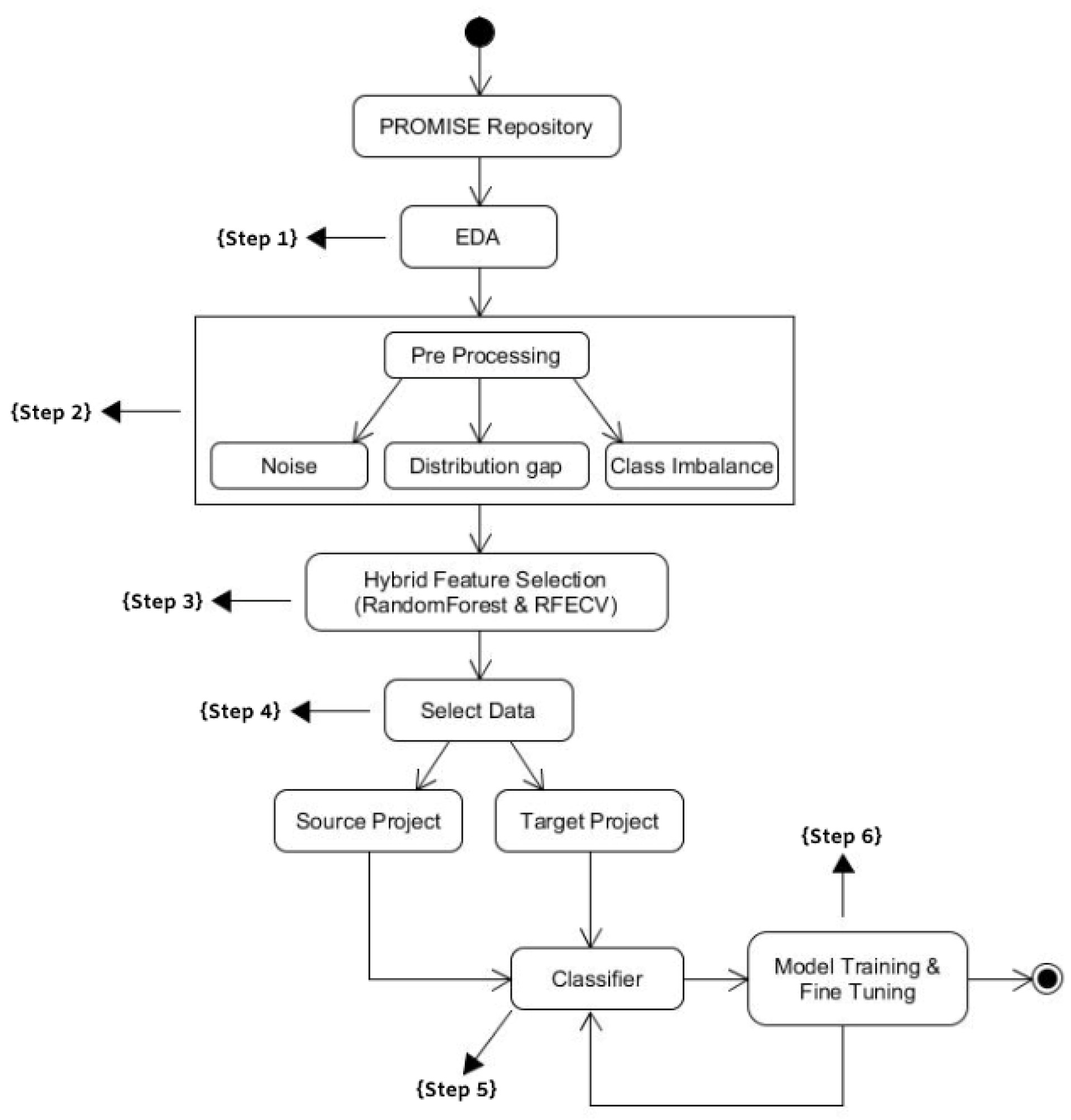
3. Proposed Methodology

Firstly, to understand our approach better, knowledge of the dataset is important. After that, we present our proposed approach, including the data normalization, architecture settings, and training process in Figure 1 below.

3.1. Exploratory Data Analysis (Step 1)

We did Exploratory Data Analysis to understand the nature of the dataset in order to normalize the data. To do so, we carried out an exploratory data analysis (EDA). Exploratory data analysis is used by data scientists to analyze and investigate datasets and summarize their main characteristics, often employing data visualization methods. It can also help determine if the statistical techniques being considered for data analysis are appropriate. We performed the experiments on one of the widely used repositories of software defect prediction: PROMISE [12,13].

Table 1. Promise repository features along with their description.

Sr. No.	Attribute	Abbreviations	Description
1	WMC	Weighted Methods per class	The number of methods used in a given class
2	DIT	Depth of Inheritance Tree	The maximum distance from a given class to the root of an inheritance tree
3	NOC	Number of Children	The number of children of a given class in an inheritance tree
4	CBO	Coupling between Object Classes	The number of classes that are coupled to a given class
5	RFC	Response for a Class	The number of distinct methods invoked by code in a given class
6	LCOM	Lack of Cohesion in Methods	The number of method pairs in a class that do not share access to any class attributes
7	CA	Afferent Coupling	Afferent coupling, which measures the number of classes that depends upon a given class
8	CE	Efferent Coupling	Efferent coupling, which measures the number of classes that a given class depends upon
9	NPM	Number of Public Methods	The number of public methods in a given class
10	LCOM3	Normalized Version of LCOM	Another type of lcom metric proposed by Henderson-Sellers
11	LOC	Lines of Code	The number of lines of code in a given class
12	DAM	Data Access Metric	The ratio of the number of private/protected attributes to the total number of attributes in a given class
13	MOA	Measure of Aggregation	The number of attributes in a given class that are of user-defined types
14	MFA	Measure of Functional Abstraction	The number of methods inherited by a given class divided by the total number of methods that can be accessed by the member methods of the given class
15	CAM	Cohesion among Methods	The ratio of the sum of the number of different parameter types of every method in a given class to the product of the number of methods in the given class and the number of different method parameter types in the whole class
16	IC	Inheritance Coupling	The number of parent classes that a given class is coupled to
17	CBM	Coupling Between Methods	The total number of new or overwritten methods that all inherited methods in a given class are coupled to
18	AMC	Average Method Complexity	The average size of methods in a given class
19	MAX_CC	Maximum Values of Methods in the same class	The maximum McCabe’s cyclomatic complexity (CC) score of methods in a given class
20	AVG_CC	Mean Values of Methods in the same class	The arithmetic means of McCabe’s cyclomatic complexity (CC) scores of methods in a given class

lists the details of the datasets as follows:

PROMISE repository consists of different datasets such as Ant, Camel, Jedit, Log4j, Ivy, Lucene, Synapse, Velocity, Xerces, Xalan, and Poi. Each dataset consists of 20 features, shown above in Table 1. There is a total of 11 projects with 35 different versions. Table 1 lists the details of the datasets.

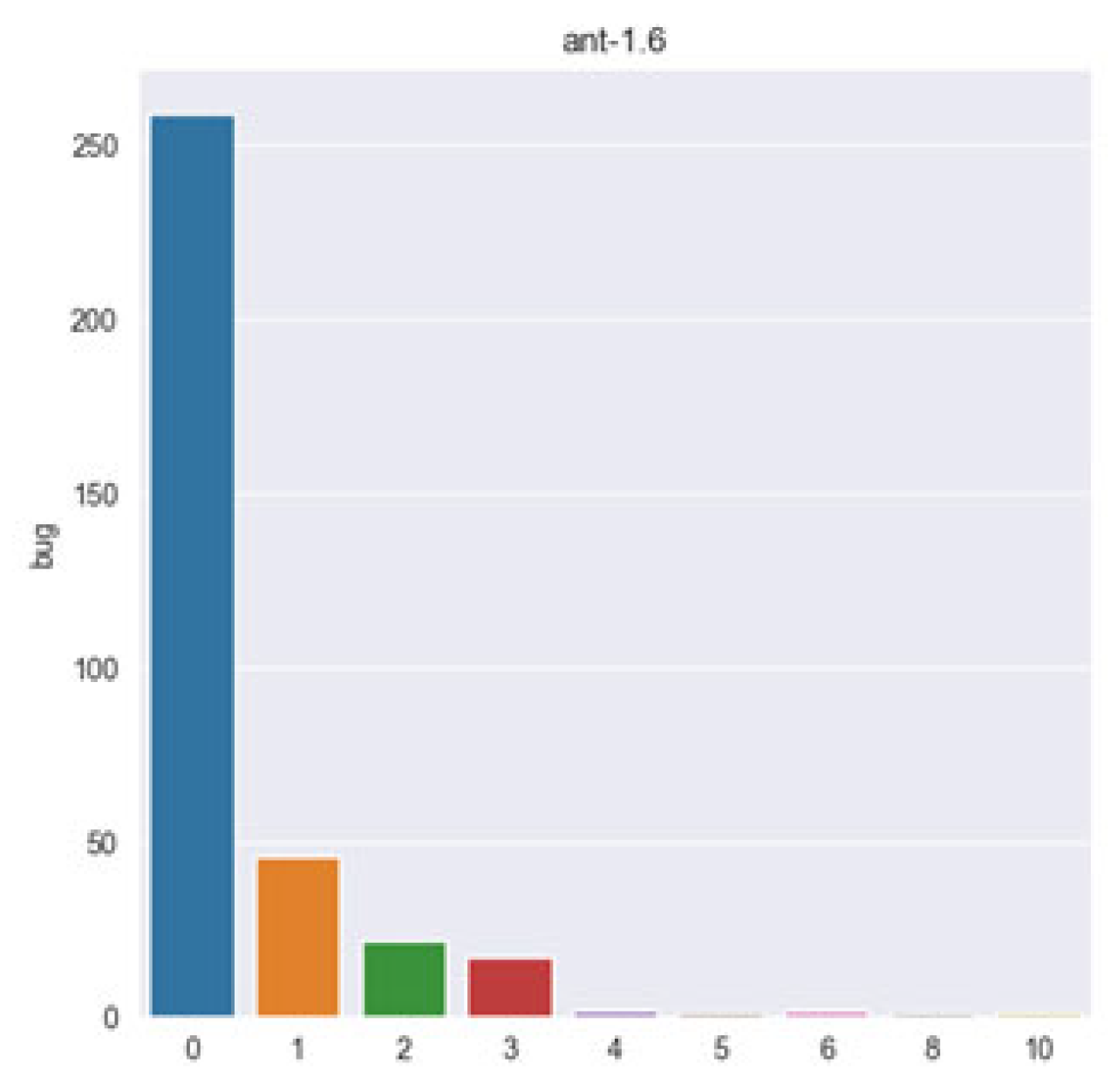
On EDA, we established that the dataset had issues of noise, data distribution gap, class imbalance issue, and had a multi-class nature. The multi-class nature of the dataset can better be described visually, as shown in the Figure 2 and Figure 3 below.

From the above diagrams, it is obvious that the promise dataset is multi-class, so we treated the dataset as multi-class during data normalization.

3.2. Data Pre-Processing (Step 2)

To normalize the dataset, we first removed the noise from the dataset. After removing noise, we covered the distribution gap between source and target projects. In the last step, we solved the issue of class imbalance by generating synthetic data. After performing all these steps, we obtained normalized data for our experimentation. Let us explain each step of data preprocessing in detail.

To answer and describe each issue, we divided our process into two steps for each, which were:

• Describing the method of performing an experiment
• Displaying the dataset before and after performing an experiment

3.2.1. Noise

The repository has noise in the form of duplicated rows. We removed noise from the PROMISE dataset by removing the redundant data, so that our trained model predicts the defects accurately with higher accuracy.

• Method to Perform Experiment

To resolve the issue of noise in the dataset, we performed the following steps:

• Read CSV File
• Drop all unimportant columns, i.e., name and version
• Use panda’s duplicated method on the data retrieved from CSV file
• Duplicating method of panda’s library, traversing each row in the dataset one by one throughout the file and selecting the duplicated rows.
• Use pandas’ method drop_duplicates on the data retrieved from the CSV file
• Use drop_duplicates method to remove all the retrieved duplicated rows from the dataset.
• Display dataset before and after performing the experiment

Figure 4 and Figure 5 display the result before and after experimenting.

From the EDA, we established that there was noise as redundant data in the rows of the dataset. This can better be explained visually as Figure 4 below:

We removed duplicated rows in the dataset in the first step of data normalization. After removing the noise, we obtained these results:

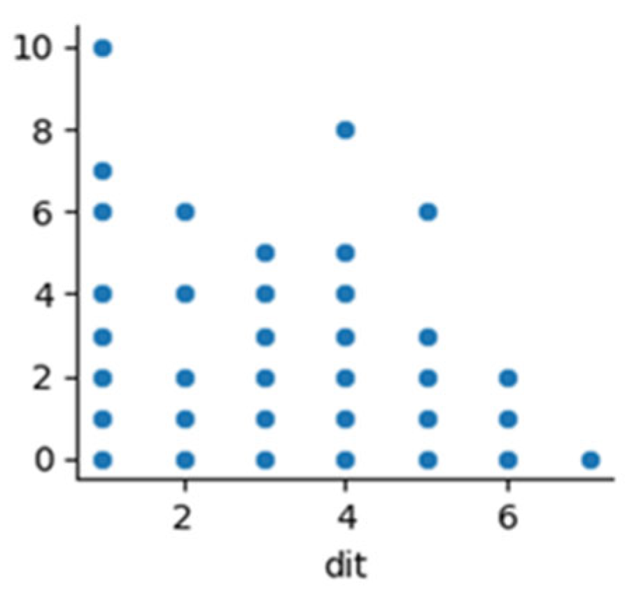
3.2.2. Distribution Gap

After removing noise, in the next step, we covered the data distribution gap in the datasets.

• Method:

To cover this gap, we used an adversarial learning concept. We first combined all the versions of datasets; in other words, we combined all the versions of Ant datasets as one CSV file and did the same for all the projects. The reason for combining all the versions is to have maximum data for training. After combining them, we had 11 different projects. We performed the following steps:

• read source CSV File
• we created a list of all the columns
• we applied a loop for each column
• we calculated minimum and maximum values based on the column
• we generated a list containing minimum and maximum range values for each column
• we removed those values which are outside the calculated min and max acceptable column values and made sure both source and target appeared in the same space.
• Dataset before and after the experiment:

Figure 6 and Figure 7 show the result before and after experimenting.

Above are the graphs of the “dit” feature of the Ant and Camel projects. We can see their distribution gap. We covered this gap using adversarial learning, in which we selected one project as the source and the other project as a target. There are two components in adversarial learning which bring source and target projects to a common space to remove the distribution gap between projects in CPDP. In adversarial learning, the generator component learns the source project. The target project is fed to the discriminator of the architecture which discriminates the source and target projects and also generates the min-max value. This min-max value will help the generator to train the source project as per the distribution of the target project. When the discriminator fails to recognize the distribution gap between the source and target project, our source project is completely trained and our source and target projects start to be situated in a common space. All the values outside the min-max value of the projects were considered outliers which we removed to cover the distribution gap completely. After removing the distribution gap, the above projects look as in Figure 8 and Figure 9 below:

Above are the graphs of the “dit” feature of Ant and Camel projects after covering the distribution gap.

3.2.3. Class Imbalance

In the last step of pre-processing, we solved the issue of class imbalance both in terms of the total number of instances and a total number of output classes. We solved the issue of class imbalance using a CTGANSynthesizer.

• Method:

To solve the class imbalance issue from the dataset, we performed the following steps:

• Once the outliers had been removed from the dataset, we used a CTGANSynthesizer. CTGAN is a collection of deep-learning-based synthetic data generators for single-table data, which can learn from real data and generate synthetic clones with high fidelity.
• We passed 100 as an epoch value as a parameter of CTGANSynthesizer to obtain the most relevant values.
• We then trained the CTGANSynthesizer model by passing data and discrete columns as parameters.
• We passed the sample size as 960, the highest number of rows in the PROMISE repository datasets. Then, using this technique, all the minority classes were oversampled to the majority class
• Dataset before and after the experiment:

Table 2. List the total number of instances for each version before resolving class imbalance. Maximum number of rows is 960 for Camel-1.6 and the minimum number of rows is 7 for Forrest-0.6.

Class Name	Total Columns	Total Rows
Camel-1.6	24	966
Xalan-2.7	24	910
Xalan-2.6	24	886
Camel-1.4	24	873
Xalan-2.5	24	804
Ant-1.7	24	746
Forest-0.8	24	33
Forest-0.7	24	30
Pbeans-1	24	27
ckjm	24	11
Forest-0.6	24	7

and

Table 3. List the total number of instances for each version after resolving the class imbalance.

Class Name	Total Columns	Total Rows
Camel-1.6	24	966
Xalan-2.7	24	966
Xalan-2.6	24	966
Camel-1.4	24	966
Xalan-2.5	24	966
Ant-1.7	24	966
Forest-0.8	24	966
Forest-0.7	24	966
Pbeans-1	24	966
ckjm	24	966
Forest-0.6	24	966

display the results before and after experimenting. All the projects have different numbers of classes in datasets as follows:

To resolve the class imbalance issue, we generated synthetic data using CTGAN. We established the maximum number of classes in any of the datasets, which was 966, and then generated all the datasets synthetically equal to 966. CTGAN learnt the dataset pattern and generated the data on the same pattern to solve the class imbalance issue.

In a detailed study about classes, we established that most of the classes of the dataset have much less data, which ultimately decreases the performance of our approach. To achieve better results, we took class 0 and class 1 as they were, but merged the classes with the bugs’ label 2, 3, 4, 5, 6, and 7 as 2. This meant that Class 2 had all kinds of bugs of classes 2, 3, 4, 5, 6, and 7. We did so to obtain the maximum data to train our model. Among the 960 classes of each of the projects, we generated equal classes for every bug class; in other words, we generated 320 classes for each of the bug class0, class1, and class2. We also balanced the classes of output.

After solving each of the issues, we obtained the normalized data for further experimentation.

3.3. Hybrid Feature Selection (Step 3)

After obtaining normalized data, we carried out feature selection to obtain the optimal feature subset for our experimentation. Hybrid methods offer a good way of combining weak feature selection methods to obtain more robust and powerful ways to select variables. Rather than using a single approach to select feature subsets as the previous methods do, hybrid methods combine the different approaches to obtain the best possible feature subset. The big advantage that hybrid methods offer is high performance and accuracy [14], better computational complexity than with wrapper methods, and models that are more flexible and robust against high dimensional data.

There are two types of hybrid feature selection, i.e., 1. Filter & Wrapper methods, and 2. Embedded and Wrapper Methods. We chose embedded and wrapper methods, which can be used to select top features, and then performed a wrapper method to rank the selected features which contribute more to the results. We used the recursive feature elimination technique to obtain our optimal feature subset. Recursive feature elimination works as follows:

• Train a model on all the data features. This model can be tree-based, lasso, or others that can offer feature importance. Evaluate its performance on a suitable metric of your choice.
• Derive the feature importance to rank features accordingly.
• Delete the least important feature and re-train the model on the remaining ones.
• Use the previous evaluation metric to calculate the performance of the resulting model.
• Now, test whether the evaluation metric decreases arbitrarily. If it does, that means this feature is important. Otherwise, you can remove it.
• Repeat steps 3–5 until all features are removed (i.e., evaluated).
• This method removes the feature only once rather than removing all the features at each step. This is why this approach is faster than pure wrapper methods and better than pure embedded methods.
• We used random forests to select the best features. We also used recursive feature elimination and cross-validation (RFECV) to rank the optimal features selected. RFECV uses different parameters for feature selection details, which are as follows:
• min_feature_to_select: as its name suggests, this parameter sets the minimum number of features to be selected.
• Step: how many features do we remove at each step?
• CV: an integer, generator, or iterable that describes the cross-validation splitting strategy.
• Scoring: the evaluation metric we use.

The dataset has a total of 20 features, as discussed in the above section, but after carrying out a hybrid feature selection, the optimal feature set came out as 14. The features ‘WMC’, ‘DIT’, ‘NOC’, ‘CBO’, ‘RFC’, ‘LCOM’, ‘CA’, ‘CE’, ‘NPM’, ‘LCOM3′, ‘LOC’, ‘DAM’, ‘MOA’, ‘MFA’, ‘CAM’, ‘IC’, ‘CBM’, ‘AMC’, ‘MAX_CC’, ‘AVG_CC’ are the 14 features selected using hybrid methods, and these features contribute the most to the results.

3.4. Dataset Division (Step 4)

After selecting features using a hybrid feature selection technique, we split the datasets into training and testing projects. Since we have less data to train our classifier, we combined all the versions of the same projects into one project and used these projects as source projects, in order to have the maximum amount of data to obtain better results. We then tested our target projects against these source projects to evaluate the prediction accuracy.

3.5. Classification (Step 5)

Data classification is carried out to obtain accuracy for our evaluation approach. To do this, we needed a classifier [15]. Since the dataset is multi-class and we were aiming to experiment on the cross-project, we added a two-layer NN which applies Softmax activation on the top of the neural network. The classifier takes the mapped instances as training data and generates a class probability as output. We used two layers of the neural network, which are the input layer and the LeakyReLU layer [15]. Using this classifier, we classified our results into Class 0, Class 1, and Class 2. We also took each of the projects as a source and target and evaluated their performance, i.e., we first took Ant as the target and all others as a source and checked the accuracies one by one. We repeated the steps by changing the target every time and by taking the rest of the projects as the source.

3.6. Model Tuning (Step 6)

We fine-tuned our model to check our results on different architectural settings. Fine-tuning of the model includes the adjustment of weights, epochs, and other parameters. By adjusting these parameters, we calculated the errors between the last output layer and the actual target layer. Fine-tuning our model helped us to identify the settings with which our model performs the best.

3.7. Research Methodology

This section describes the detailed facts of our study. All the sections for both the research questions remained the same except for independent variables and design. The content is discussed in detail.

3.7.1. Context

The context of our research is cross-project defect prediction. We predicted the defects in cross-project using the neural network layer.

3.7.2. Data Collection

The dataset consists of numeric and statistical data, so our research used quantitative research methods to collect data, as quantitative research methods focus on numbers and statistics. We used the numeric datasets of different projects of the PROMISE repository as input to our approach for training our model. In our research, we normalized the datasets before training our model (e.g., removing noise, and class imbalance issues and covering the distribution gap between source and target projects).

3.7.3. Research Type

The research type of our approach is explanatory. The objective of explanatory research is to explain the causes and consequences of a well-defined problem. Cross-project defect prediction is a well-defined problem. We found the defect prediction accuracy using hybrid feature selection and layers of neural network, to which SoftMax activation layer was applied as a classifier.

3.7.4. Research Method

Our research is based on an experimental research method to manipulate and control variables in order to determine cause and effect between variables for prediction accuracy and authenticity. Our research method consists of the following sub-sections.

• Perspective

The perspective of our experiment is the earlier defect prediction based on already developed non-defective projects. Through our experiment, we predicted the defects earlier by training our model using trained source projects and then testing our trained model in the target projects.

• Purpose

The purpose of our experiment is to evaluate the impact of optimal feature selection through hybrid feature selection in neural networks for cross-project defect prediction, and to achieve higher defect prediction accuracy by getting optimal features through hybrid feature selection after normalizing data by removing noise, solving class imbalance issues, and covering the distribution gap between source and target projects of the PROMISE Repository.

• Object of study

We set projects of the PROMISE Repository as source and target projects which are the objects of the study.

• Dependent variables

Our research has accuracy (AUC) as the dependent variable.

• Statistical Analysis

Our research will use the Wilcoxon test for cross-project defect prediction authenticity as statistical analysis.

• Independent variables for RQ1

Our research has NN as a manipulative independent variable.

• Design for RQ1

Our research design is IF1T (1 factor 1 treatment).

• Factor- Design Method
• Treatment

1. NN

3.8. Research Question

According to our literature review, research summary, and research gap, we addressed the following questions in our research paper:

RQ1:

What is the impact of hybrid feature selection in multi-class for the cross-project defect prediction accuracy of the PROMISE repository?

Null Hypothesis (H0):

Hybrid feature selection has no impact on multi-class in predicting cross-project defect prediction accuracy of the PROMISE repository.

Alternate Hypothesis (H1):

Hybrid feature selection has an impact on multi-class in predicting cross-project defect prediction accuracy of the PROMISE repository.

4. Result and Analysis

In this section, we will answer our research question and will also analyze our results. The research question addressed is as follows:

4.1. Hyper-Parameter Tuning

We fine-tuned hyper-parameters by adjusting our learning rate, epochs, and neural network layers to get the optimal hyper-parametric settings for defect prediction. Details are:

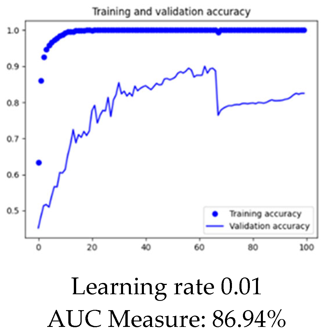
4.1.1. Learning Rate

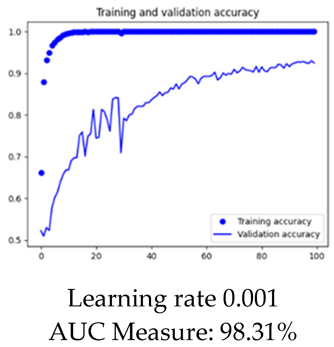
We took Ant as the target project and Log4j as the source project to see the impact of fine-tuning on learning rate. We performed the same experiment on a learning rate of 0.1, 0.01, and 0.001. The Figure 10, Figure 11 and Figure 12 below show the visualization of results for each learning rate.

From the above visualization in Figure 10, Figure 11 and Figure 12, it is clear that the optimized learning rate for the project is 0.01.

4.1.2. Epochs

To set the epochs for the experiment, we took Ant as the target project and Log4j as the source project to see the impact of fine-tuning epochs. We performed the same experiment on epochs 30, 100, and 200. The Figure 13, Figure 14 and Figure 15 below show the visualization of results for each of the epochs.

From the above visualization in Figure 13, Figure 14 and Figure 15, it is clear that the set of epochs for the project should be 100, so we set 100 epochs for all the projects throughout the experiment except the log4j and Ivy. For Log4j as the target and all others as the source, epochs vary from 200–500. Similarly, for Ivy as the target project, epochs for every other source project vary from 300–500 due to having less data for training.

4.1.3. Neural Network Layers

We took Ant as the target project and Log4j as the source project to see the impact of adding dense layers to our architecture. We performed the same experiment on dense layers at 16, 32, and 64. The Figure 16, Figure 17 and Figure 18 below show the visualization of results for each of the dense layer settings.

From the above visualization in Figure 16, Figure 17 and Figure 18, it is clear that the optimized dense layers for the project are 32, so we set dense layers as 32 for all the projects throughout the experiment.

4.2. Experimental Configuration

Experimental configurations of our experiment were as follows:

• Batch Size: 64
• Epochs: We set the epochs for almost every project as 100 but for a smaller number of training datasets. We also set epochs to be 200 or 300.
• Optimizer: Adam (learning rate = 0.001)
• Activation Function: SoftMax
• Hybrid feature selection method and neural network model architecture is shown in below Figure 19

In this study, the number of epochs was set to 100, except for some of the projects with fewer data issues, and the time cost was less than 60 s for every target project which was run.

4.3. Results and Analysis

In this section, we will answer our research question and will also analyze our results. The research question addressed was as follows:

RQ1:

What is the impact of hybrid feature selection in multi-class for the cross-project defect prediction accuracy of the PROMISE repository?

To answer this question in our research, we performed a controlled experiment on open-source projects of the PROMISE repository and evaluated the results in terms of AUC measure. We first normalized the dataset by removing noise, covering the distribution gap, and solving the class imbalance issue. The PROMISE repository consists of 28 datasets of many versions of 11 different projects. We combined all the versions of each of the datasets as one project to increase the dataset, in order to improve the training of our model. We then used the hybrid feature selection method to obtain the optimal feature subset that contributes the most to defect prediction. After obtaining the optimal features, we evaluated the accuracy of our model in terms of AUC measure by using two layered neural networks with a SoftMax Activation layer on the top as a classifier to classify the results in class0, class1, and class2.

We have displayed our results for each of the target and source projects of the repository and evaluate the results in AUC measure as follows in

Table 4. Results of Experiment in AUC Measure for each target project.

AUC Measure
Source
Target	Ant	Camel	Jedit	Lucene	Poi	Log4j	Velocity	Synapse	Ivy	Xalan	Xerces
Ant-1.3	--	62.91%	62.66%	63.07%	65.32%	60.47%	53.50%	62.74%	66.80%	66.60%	61.76%
Ant-1.4	--	50.68%	70.76%	73.83%	69.82%	60.27%	64.39%	71.46%	69.65%	66.23%	52.89%
Ant-1.5	--	77.46%	75.37%	67.92%	75.48%	69.02%	34.68%	66.47%	65.80%	71.31%	78.16%
Ant-1.7	--	76.78%	78.60%	76.68%	72.54%	60.42%	63.03%	84.77%	79.42%	83.23%	72.83%
Camel-1.2	70.81%	--	66.78%	75.96%	68.92%	70.80%	52.87%	70.46%	66.63%	62.28%	59.19%
Camel-1.4	80.96%	--	69.12%	77.40%	74.60%	67.37%	63.21%	71.13%	75.48%	69.26%	60.98%
Camel-1.6	78.86%	--	74.52%	72.80%	69.96%	64.63%	57.64%	69.05%	76.62%	70.00%	72.55%
Ivy-2.0	84.08%	72.62%	78.26%	76.29%	75.13%	64.12%	62.46%	76.02%	--	77.92%	74.62%
Jedit-3.2	83.90%	74.48%	--	71.33%	76.68%	62.43%	59.35%	79.11%	81.10%	72.01%	69.81%
Jedit-4.0	86.05%	77.30%	--	76.90%	64.95%	62.33%	65.40%	84.83%	82.67%	64.50%	53.62%
Jedit-4.1	80.75%	71.28%	--	66.51%	65.26%	58.24%	48.99%	71.39%	82.65%	77.54%	58.00%
Log4j-1.0	80.68%	76.86%	73.98%	75.23%	71.62%	--	66.16%	64.75%	73.01%	65.80%	60.53%
Log4j-1.1	86.09%	77.48%	75.36%	78.90%	69.61%	--	62.16%	72.47%	58.60%	71.52%	60.10%
Log4j-1.2	61.99%	66.25%	58.96%	65.82%	53.89%	--	50.55%	59.68%	49.38%	56.86%	48.24%
Lucene-2.0	74.84%	69.11%	63.11%	--	66.82%	56.62%	57.70%	71.58%	75.04%	65.88%	54.75%
Lucene-2.2	65.98%	61.37%	66.38%	--	66.24%	61.59%	55.50%	65.02%	66.61%	60.47%	55.59%
Lucene-2.4	68.31%	64.91%	66.50%	--	62.42%	66.92%	58.11%	63.65%	62.04%	62.21%	53.58%
Synapse-1.0	88.08%	65.65%	64.03%	65.82%	78.39%	49.82%	59.50%	--	77.69%	75.36%	49.59%
Synapse-1.1	74.45%	71.04%	74.07%	64.73%	69.38%	57.49%	57.98%	--	73.42%	62.96%	63.15%
Synapse-1.2	72.65%	65.63%	61.25%	62.15%	65.05%	59.05%	61.39%	--	72.36%	66.82%	58.91%
Velocity-1.4	61.64%	53.99%	59.91%	63.86%	61.13%	64.92%	--	66.89%	63.72%	59.26%	58.75%
Velocity-1.5	68.99%	60.81%	77.47%	73.42%	68.40%	61.90%	--	71.65%	65.47%	64.60%	64.43%
Velocity-1.6	56.93%	55.34%	57.90%	58.05%	63.65%	48.25%	--	65.30%	63.87%	51.56%	51.45%
Xalan-2.4	72.63%	69.76%	69.86%	65.40%	67.00%	57.75%	56.21%	69.51%	76.31%	--	64.72%
Xalan-2.5	79.00%	78.57%	74.75%	69.07%	73.39%	58.82%	55.21%	74.44%	78.51%	--	60.88%
Xalan-2.6	77.25%	70.32%	71.56%	68.36%	64.83%	59.30%	51.37%	73.86%	76.62%	--	67.41%
Xerces-1.2	63.35%	64.73%	60.31%	55.35%	60.20%	54.14%	53.95%	65.14%	66.32%	54.75%	--
Xerces-1.4	63.71%	64.76%	64.55%	63.91%	61.74%	62.79%	50.11%	59.23%	60.14%	64.96%	--

:

The above Table 4 show the results of our experiment, which we established by finding the impact of the NN classifier along with the SoftMax layer. The SoftMax layer performs the best when it comes to multi-class datasets because of its output probability range, which is from 0 to 1, and the sum of all probabilities is equal to 1.

Using EDA, we established that the dataset had 63 output classes in which the majority of the instances were 0 and 1 classes. Instances greater than 1 were so few in number that we put them all in class 2. The reason was that to have the maximum amount of data for training our model, we used CTGAN to generate synthetic data. CTGAN trains the classifier based on several instances and then generates the synthetic data on the pattern of already existing classes. CTGAN learns the pattern and generates data where greater number of data is required. All the classes above 1 were fewer in number and CTGAN finds it difficult to generate the synthetic data with less data. To overcome this issue, we combined all the classes above 1 in a single class 2.

To experiment, we combined all the versions of the same dataset as one project and treated it as the source. We then tested one source project against all the versions of 28 projects from the promise repository. We combined the versions to get a large range of data so that we could efficiently train our classifier. By combining the versions of one project, we also obtained the maximum range of the project to train our classifier.

Table 4 shows the results we obtained from our experiment. We have highlighted the highest accuracy of one project in bold in every row. In Table 4, where source and target are same, we put dashes at their intersection point because we aren’t addressing the issue of WPDP. As our experimental domain is cross-project defect prediction, we did not predict the results for the same target projects.

From our experimental results, it is evident that through hybrid feature selection we obtained the optimal set of features. By combining the SoftMax layer with the NN layer, better prediction accuracies were achieved for a multi-class dataset in terms of AUC measure for the PROMISE repository, which supports our alternative hypothesis, i.e., “Hybrid feature selection selects optimal feature sets for multi-class in predicting cross-project defect prediction accuracy of PROMISE repository”.

4.4. Research Validation

We validated our results with two statistical tests i.e., the Wilcoxon Test. Details are as follows:

4.4.1. Wilcoxon Test

“The Wilcoxon signed ranks test is a nonparametric statistical procedure for comparing two samples that are paired, or related. The parametric equivalent to the Wilcoxon signed ranks test goes by names such as the student’s t-test, t-test for matched pairs, t-test for paired samples, or t-test for dependent samples”.

4.4.2. Hypothesis Assumption

The following are the assumptions for the hypothesis:

• Observations in each sample are independent and identically distributed (iid).
• Observations in each sample can be ranked.

4.4.3. Acceptance Criteria

The significance level, based on the information provided, is alpha = 0.05. If the p-value is greater than alpha, then H0 is accepted, otherwise it is rejected.

4.4.4. Test Statistics

Table 5. Test statistics of Wilcoxon test.

Test Statistics
	p-Value	Accepted Hypothesis
Wilcoxon Test	0.0039	H1

shows the test results using the Wilcoxon test. We calculated the value of p by passing two groups in the Wilcoxon test. We considered Ant as a target project and observed the accuracy with other source projects i.e., Ivy, Camel, Synapse, Velocity, Lucene, Poi, Xerces, Xalan, and Log4j. One of the groups of the observation contained values of measure without applying hybrid feature selection and another observation contained values of the measure after applying hybrid feature selection.

4.4.5. Analysis of Validation Test

The above Table 5 shows that our alternative hypothesis was approved, which clearly shows that our approach of hybrid feature selection in neural networks does have an impact on the cross-project defect prediction.

5. Threat to Validity

During an empirical study, one should be aware of the potential threats to the validity of the obtained results and derived conclusions. The potential threats to the validity identified for this study are divided into three categories, namely: internal, external, and construct validity.

5.1. Internal Validity

We implemented the baselines by carefully following the base papers [1,2]. These compared related works did not provide the source codes of their works, so we did not work on the source code of the dataset. We worked on the static features of the dataset.

5.2. External Validity

PROMISE datasets used for validation are open-source software project data. If our proposed approach were built on closed software projects developed under different environments, it might produce better/worse performance.

5.3. Construct Validity

We mainly used AUC-measure, which has been widely used to evaluate the effectiveness of defect prediction models, to evaluate the prediction performance. On the other hand, the experimental datasets were collected by Jureczko et al., who cautioned that there could be some mistakes in non-defective labels as not all the defects had been found. This may be a potential threat to defect prediction model training and evaluation [16].

6. Conclusions

Using EDA, we established that the PROMISE dataset was multi-class, which has noise, distribution gap, and class imbalance issues, as clearly shown above in Figure 2, Figure 4, Figure 5, Figure 7 and Figure 8, and Table 3. From our experimental results, it is evident that after removing noise, covering the distribution gap and balancing the classes, and selecting optimal features set using the hybrid feature selection technique, we can obtain better results. We used the NN classifier along with the Softmax layer to predict the accuracy of our experiment as the SoftMax layer has proved to perform better for multi-class classification. We predicted the accuracy for all 28 versions of all 11 projects in terms of AUC measure, with an average of 75.96%. We validated our results using the Wilcoxon test. Our experimental results clearly illustrate that CPDP can help to predict the defects in software modules and will help in the early prediction of defects.

References

- Sun, Y.; Jing, X.Y.; Wu, F.; Li, J.; Xin, D.; Chen, H.; Sun, Y. Adversarial Learning for Cross-Project Semi-Supervised Defect Prediction. IEEE Access 2020, 8, 32674–32687. [Google Scholar] [CrossRef]
- Hosseini, S.; Turhan, B.; Mäntyl, M. A benchmark study on the effectiveness of search-based data selection and feature selection for cross-project defect prediction. Inf. Softw. Technol. 2018, 95, 296–312. [Google Scholar] [CrossRef]
- Yu, Q.; Qian, J.; Jiang, S.; Wu, Z.; Zhang, G. An Empirical Study on the Effectiveness of Feature Selection for Cross Project Defect Prediction. IEEE Access 2019, 7, 35710–35718. [Google Scholar] [CrossRef]
- Kumar, R.P.; Varma, S.D.G. A novel multi-level based cross defect prediction model for multiple software defect databases. Int. J. Pure Appl. Math. 2017, 117, 293–301. [Google Scholar]
- Ryu, D.; Jang, J.-I.; Baik, J. A Hybrid Instance Selection Using Nearest-Neighbor for Cross-Project Defect Prediction. J. Comput. Sci. Technol. 2015, 30, 969–980. [Google Scholar] [CrossRef]
- Alqahtani, H.; Kavakli-Thorne, M.; Kumar, G. Applications of Generative Adversarial Networks (GANs): An Updated Review. Arch. Comput. Methods Eng. 2021, 28, 525–552. [Google Scholar] [CrossRef]
- Xu, L.; Veeramachaneni, K. Synthesizing tabular data using GAN. arXiv 2018, arXiv:1811.11264. [Google Scholar] [CrossRef]
- Park, N.; Mohammadi, M.; Gorde, K. Data Synthesis based on Generative Adversarial Networks. Proc. VLDB Endow. 2018, 11, 1071–1083. [Google Scholar] [CrossRef]
- Quintana, M.; Miller, C. Towards Class-Balancing Human Comfort Datasets with GANs. In Proceedings of the 6th ACM International Conference on Systems for Energy-Efficient Buildings, Cities, and Transportation, New York, NY, USA, 13–14 November 2019; pp. 391–392. [Google Scholar] [CrossRef]
- Khoshgoftaar, M.T.; Gao, K.; Seliya, N. Attribute Selection and Imbalanced Data: Problems in Software Defect Prediction. In Proceedings of the 22nd IEEE International Conference on Tools with Artificial Intelligence, Arras, France, 27–29 October 2010; Volume 1, pp. 137–144. [Google Scholar] [CrossRef]
- Bejjanki, K.K.; Gyani, J.; Gugulothu, N. Class Imbalance Reduction (CIR): A Novel Approach to Software Defect Prediction in the Presence of Class Imbalance. Symmetry 2020, 12, 407. [Google Scholar] [CrossRef]
- Sayyad Shirabad, J.; Menzies, T.J. PROMISE Software Engineering Repository. Available online: http://promise.site.uottawa.ca/SERepository (accessed on 1 January 2022).
- Rodriguez, D.; Herraiz, I.; Harrison, R. On Software Engineering Repositories and Their Open Problems. In Proceedings of the First International Workshop on Realizing AI Synergies in Software Engineering (RAISE), Zurich, Switzerland, 5 June 2012; pp. 52–56. [Google Scholar] [CrossRef]
- Fallah, S.N.; Deo, R.C.; Shojafar, M.; Conti, M.; Shamshirband, S. Computational Intelligence Approaches for Energy Load Forecasting in Smart Energy Management Grids: State of the Art, Future Challenges, and Research Directions. Energies 2018, 11, 596. [Google Scholar] [CrossRef]
- Shepperd, M.; Bowes, D.; Hall, T. The Use of Machine Learning in Software Defect Prediction. IEEE Trans. Softw. Eng. 2014, 40, 603–616. [Google Scholar] [CrossRef]
- Menzies, T.; Milton, Z.; Turhan, B.; Cukic, B.; Jiang, Y.; Bener, A. Defect prediction from static code features current results, limitations, new approaches. Autom. Softw. Eng. 2010, 17, 375–407. [Google Scholar] [CrossRef]
Figure 1.
Our proposed methodology.
Figure 2.
Multi-class of project ant 1.6.
Figure 3.
Multi-Class of project Xerces 1.4.
Figure 4.
Noise in terms of duplicated records in ant version 1.3.
Figure 5.
Removed noise in terms of duplicated records in ant version 1.3.
Figure 6.
Before removing the data distribution of the “dit” feature of the Ant project.
Figure 7.
Before removing the data distribution of the “dit” feature of the Camel project.
Figure 8.
After removing the data distribution of the “dit” feature of the Ant project.
Figure 9.
After removing the data distribution of the “dit” feature of the Camel project.
Figure 10.
Graphical representation of model at learning rate 0.1.
Figure 11.
Graphical representation of model at learning rate 0.01.
Figure 12.
Graphical representation of model at learning rate 0.001.
Figure 13.
Graphical representation of model at Epochs 30.
Figure 14.
Graphical representation of model at Epochs 100.
Figure 15.
Figure 16.
Graphical representation of model with Dense Layer 16.
Figure 17.
Graphical representation of model with Dense Layer 32.
Figure 18.
Graphical representation of model with Dense Layer 64.
Figure 19.
Experimental configuration of our model.