
Imitative Reinforcement Learning Fusing Mask R-CNN Perception Algorithms


Abstract
:1. Introduction
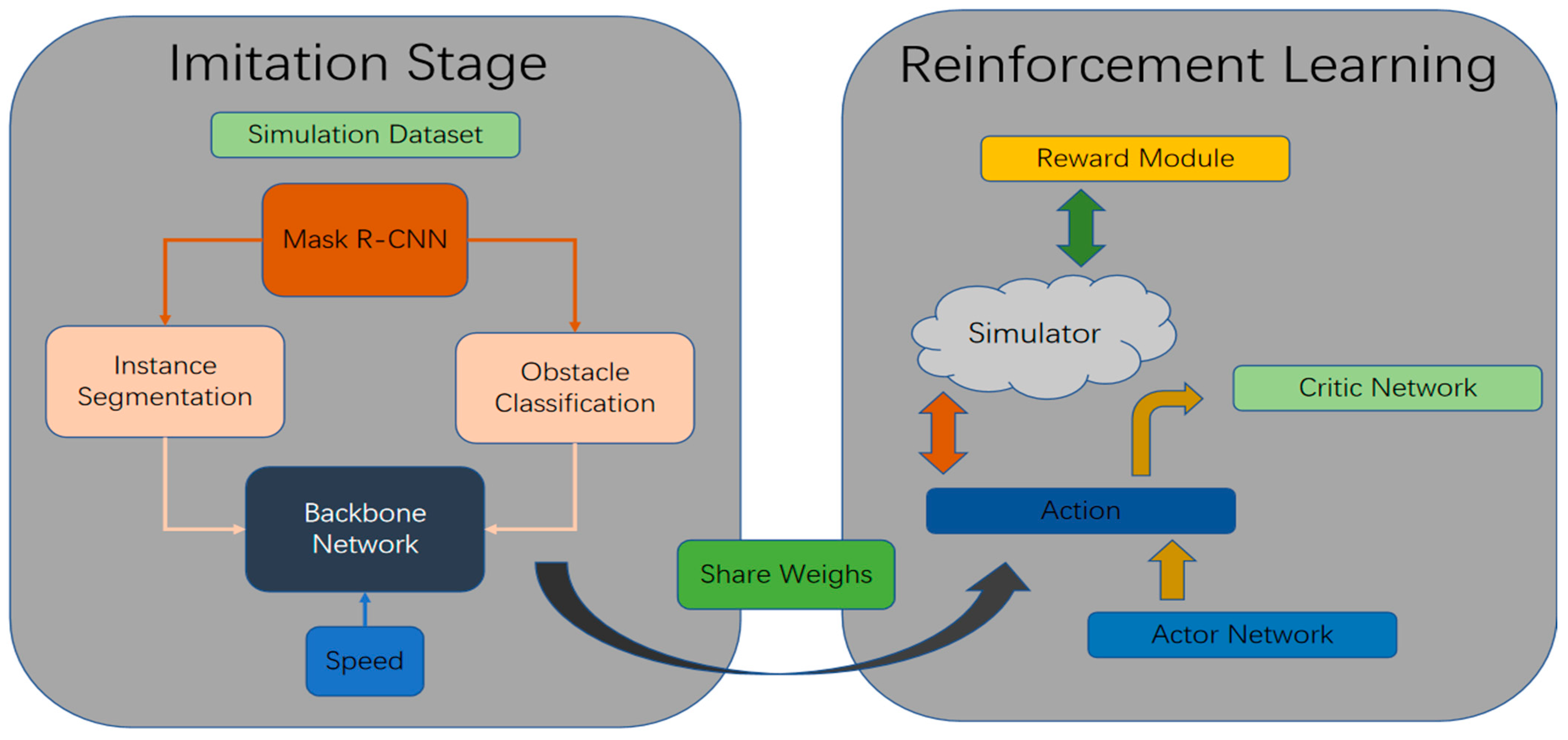
- This paper proposes a two-stage framework called CIL-DDPG, which combines reinforcement learning and imitation learning using obstacle position information as additional input, and Mask-RCNN [10] is used for image segmentation. The collection of CIL and DDPG is an innovative development; previous releases have used the two methods separately as one development algorithm; secondly, this paper has made innovations such as obstacle information fusion in CIL.
- A new reward function is designed to learn an alternative autonomous driving strategy in a dynamic scenario. Extensive experiments on the CARLA simulator benchmark show that the work in this paper enables the network to overcome the effects of image noise.
2. Related Work
3. Mask R-CNN
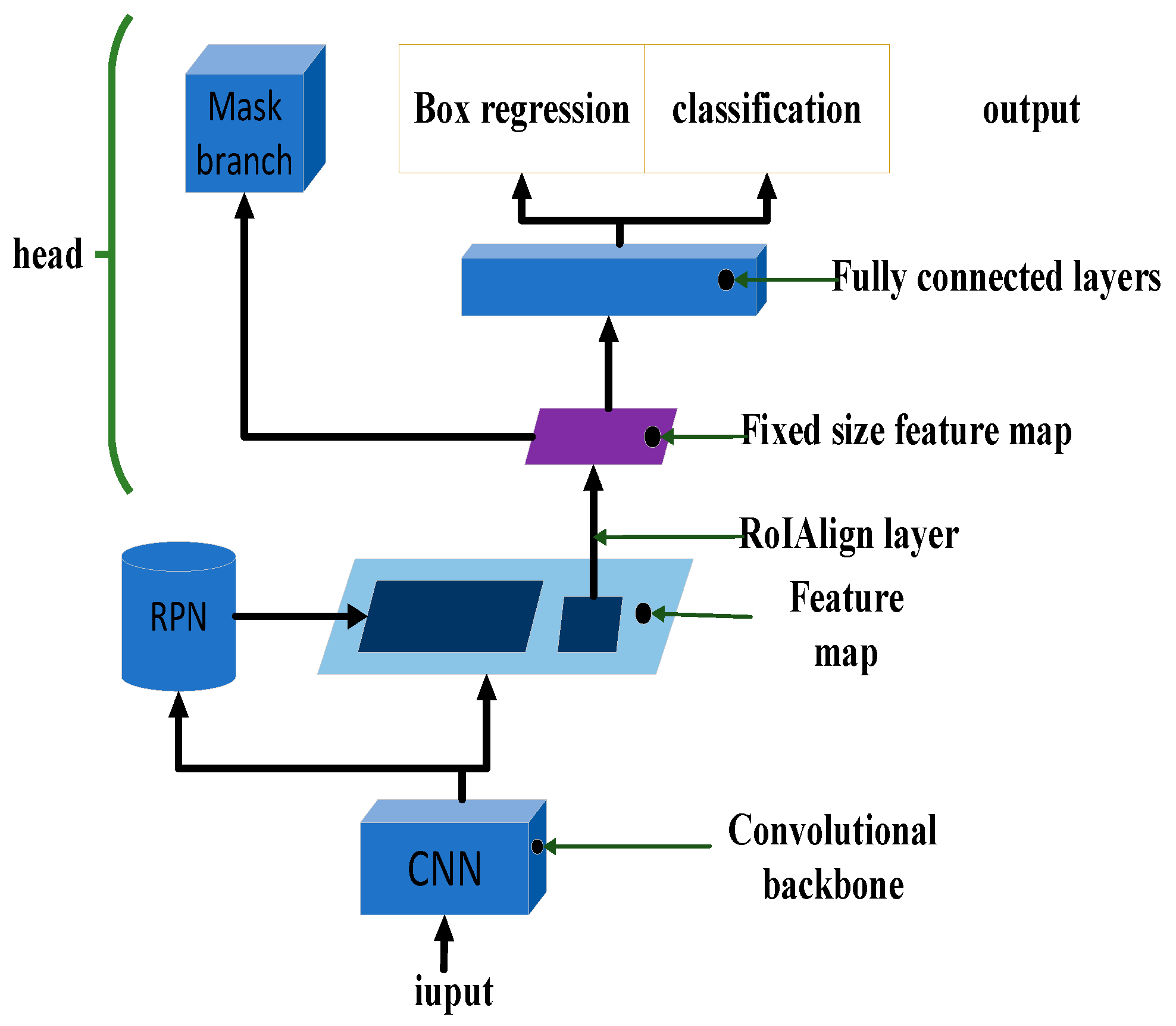
3.1. Structure of Mask R-CNN
| Algorithm 1. Mask-RCNN |
| Input: the RGB images Output: Image with category, mask and bounding box Repeat: until there is no rgb image input Step 1: The RGB images are fed into ResNet101 for feature fusion; Step 2: Then two feature maps are generated as rpn_feature_maps and mrcnn_feature_maps; Step 3: Different sizes of rpn_feature_maps are sent to the RPN in the feature extraction phase; Step 4: After the RPN, the rpn_class, rpn_box and the anchor generator generated from the anchors, finally go to the Proposal Layer; Step 5: Mapping proposals of mrcnn_class, mrcnn_bboxes and iuput_image_meta to the final layer of the DetectionTargetLayer; Step 6: Generating a fixed-size feature map for each RoI using an RoI Align layer; Step 7: The detections are combined with mrcnn_feature_maps to fpn_mask_graph; Step 8: Final generation of mrcnn_masks. End repeat |
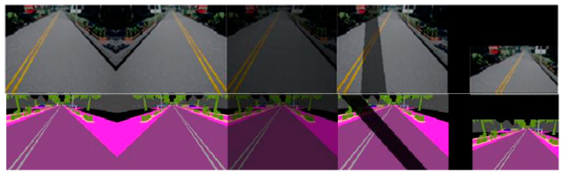
3.2. Dataset Acquisition
3.3. Image Enhancement
4. Imitation Learning
4.1. Conditional Imitation Learning
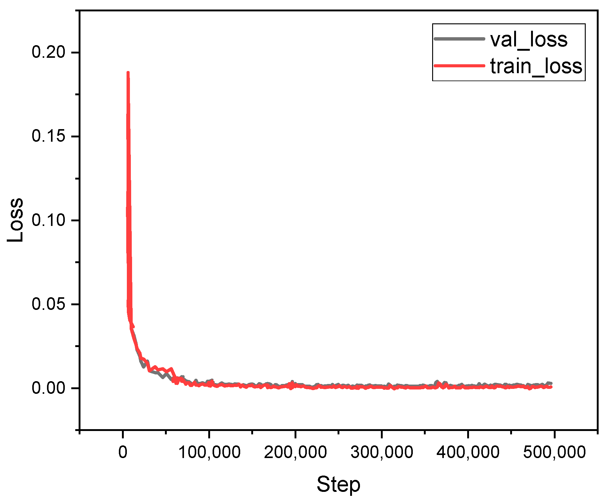
4.2. Training and Validation
5. Reinforcement Learning
5.1. Markov Decision Process (MDP)
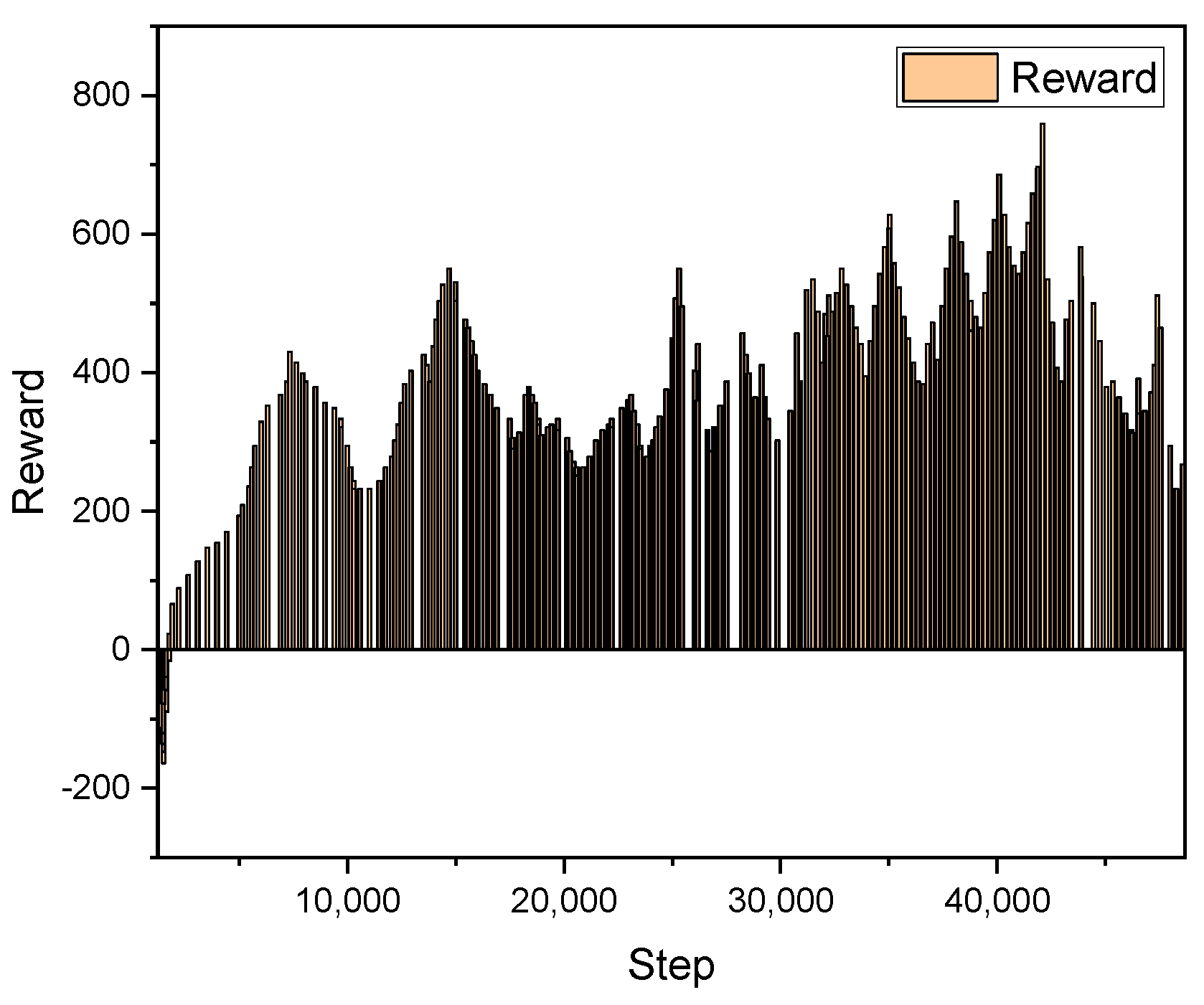
5.2. Reward Function of DDPG
6. Simulation Experiments
6.1. Experimental Settings
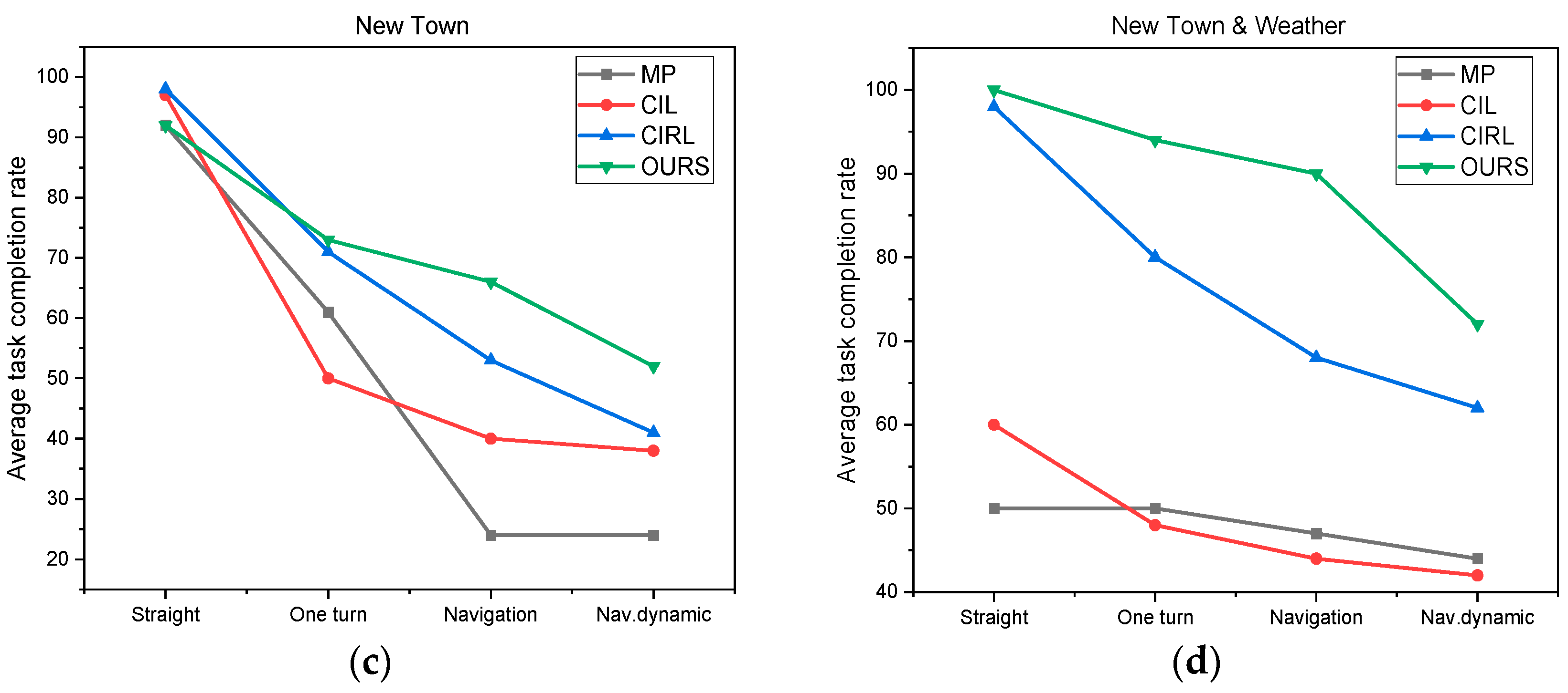
6.2. Results
7. Conclusions
Author Contributions
Funding
Institutional Review Board Statement
Informed Consent Statement
Data Availability Statement
Conflicts of Interest
References
- Chen, C.; Seff, A.; Kornhauser, A.; Xiao, J. Deepdriving: Learning affordance for direct perception in autonomous driving. In Proceedings of the IEEE International Conference on Computer Vision, Santiago, Chile, 7–13 December 2015; pp. 2722–2730. [Google Scholar]
- Heess, N.; TB, D.; Sriram, S.; Lemmon, J.; Merel, J.; Wayne, G.; Tassa, Y.; Erez, T.; Wang, Z.; Ali Eslami, S.M.; et al. Emergence of locomotion behaviours in rich environments. arXiv 2017, arXiv:1707.02286. [Google Scholar]
- Tian, Y.; Pei, K.; Jana, S.; Ray, B. Deeptest: Automated testing of deep-neural-network-driven autonomous cars. In Proceedings of the 40th International Conference on Software Engineering, Gothenburg, Sweden, 27 May–3 June 2018; pp. 303–314. [Google Scholar]
- Tariq, A.; Osama, S.M.; Gillani, A. Development of a low cost and light weight uav for photogrammetry and precision land mapping using aerial imagery. In Proceedings of the 2016 International Conference on Frontiers of Information Technology (FIT), Como, Italy, 16–19 May 2016; pp. 360–364. [Google Scholar]
- Von Bernuth, A.; Volk, G.; Bringmann, O. Simulating photo-realistic snow and fog on existing images for enhanced CNN training and evaluation. In Proceedings of the 2019 IEEE Intelligent Transportation Systems Conference (ITSC), Auckland, New Zealand, 27–30 October 2019; pp. 41–46. [Google Scholar]
- Liang, X.; Zhang, J.; Zhuo, L.; Li, Y.; Tian, Q. Small object detection in unmanned aerial vehicle images using feature fusion and scaling-based single shot detector with spatial context analysis. IEEE Trans. Circuits Syst. Video Technol. 2019, 30, 1758–1770. [Google Scholar] [CrossRef]
- Faisal, M.M.; Mohammed, M.S.; Abduljabar, A.M.; Abdulhussain, S.H.; Mahmmod, B.M.; Khan, W.; Hussain, A. Object Detection and Distance Measurement Using AI. In Proceedings of the 2021 14th International Conference on Developments in eSystems Engineering (DeSE), Sharjah, United Arab Emirates, 7–10 December 2021; pp. 559–565. [Google Scholar] [CrossRef]
- Dosovitskiy, A.; Ros, G.; Codevilla, F.; Lopez, A.; Koltun, V. CARLA: An open urban driving simulator. In Proceedings of the Conference on Robot Learning, Mountain View, CA, USA, 13–15 November 2017; PMLR. pp. 1–16. [Google Scholar]
- Codevilla, F.; Santana, E.; López, A.M.; Gaidon, A. Exploring the Limitations of Behavior Cloning for Autonomous Driving. In Proceedings of the 2019 IEEE/CVF International Conference on Computer Vision (ICCV), Seoul, Republic of Korea, 27 October–2 November 2019; pp. 9328–9337. [Google Scholar]
- He, K.; Gkioxari, G.; Dollár, P.; Girshick, R. Mask r-cnn. In Proceedings of the IEEE International Conference on Computer Vision, Venice, Italy, 22–29 October 2017; pp. 2961–2969. [Google Scholar]
- Lillicrap, T.P.; Hunt, J.J.; Pritzel, A.; Heess, N.; Erez, T.; Tassa, Y.; Silver, D.; Wierstra, D. Continuous control with deep reinforcement learning. arXiv 2015, arXiv:1509.02971. [Google Scholar] [CrossRef]
- Michaelis, C.; Mitzkus, B.; Geirhos, R.; Rusak, E.; Bringmann, O.; Ecker, A.S.; Bethge, M.; Brendel, W. Benchmarking robustness in object detection: Autonomous driving when winter is coming. arXiv 2019, arXiv:1907.07484. [Google Scholar] [CrossRef]
- Tomy, A.; Paigwar, A.; Mann, K.S.; Renzaglia, A.; Laugier, C. Fusing Event-based and RGB camera for Robust Object Detection in Adverse Conditions. In Proceedings of the 2022 International Conference on Robotics and Automation (ICRA), Philadelphia, PA, USA, 23–27 May 2022; pp. 933–939. [Google Scholar] [CrossRef]
- Boisclair, J.; Kelouwani, S.; Ayevide, F.K.; Amamou, A.; Alam, M.Z.; Agbossou, K. Attention transfer from human to neural networks for road object detection in winter. IET Image Process. 2022, 16, 3544–3556. [Google Scholar] [CrossRef]
- Simonyan, K.; Zisserman, A. Very deep convolutional networks for large-scale image recognition. arXiv 2014, arXiv:1409.1556. [Google Scholar] [CrossRef]
- He, K.; Zhang, X.; Ren, S.; Sun, J. Deep residual learning for image recognition. In Proceedings of the IEEE Conference on Computer Vision and Pattern Recognition, Las Vegas, NV, USA, 27–30 June 2016; pp. 770–778. [Google Scholar]
- Long, J.; Shelhamer, E.; Darrell, T. Fully convolutional networks for semantic segmentation. In Proceedings of the IEEE Conference on Computer Vision and Pattern Recognition, Boston, MA, USA, 7–12 June 2015; pp. 3431–3440. [Google Scholar]
- Zhang, B.; Zhang, J. A traffic surveillance system for obtaining comprehensive information of the passing vehicles based on instance segmentation. IEEE Trans. Intell. Transp. Syst. 2020, 22, 7040–7055. [Google Scholar] [CrossRef]
- Bojarski, M.; del Testa, D.; Dworakowski, D.; Firner, B.; Flepp, B.; Goyal, P.; Jackel, L.D.; Monfort, M.; Muller, U.; Zhang, J.; et al. End to end learning for self-driving cars. arXiv 2016, arXiv:1604.07316. [Google Scholar] [CrossRef]
- Bojarski, M.; Yeres, P.; Choromanska, A.; Choromanski, K.; Firner, B.; Jackel, L.; Muller, U. Explaining how a deep neural network trained with end-to-end learning steers a car. arXiv 2017, arXiv:1704.07911. [Google Scholar] [CrossRef]
- Eraqi, H.M.; Moustafa, M.N.; Honer, J. End-to-end deep learning for steering autonomous vehicles considering temporal dependencies. arXiv 2017, arXiv:1710.03804. [Google Scholar] [CrossRef]
- Codevilla, F.; Müller, M.; López, A.; Koltun, V.; Dosovitskiy, A. End-to-end driving via conditional imitation learning. In Proceedings of the 2018 IEEE International Conference on Robotics and Automation (ICRA), Brisbane, Australia, 21–25 May 2018; pp. 4693–4700. [Google Scholar]
- Wang, Q.; Chen, L.; Tian, W. End-to-end driving simulation via angle branched network. arXiv 2018, arXiv:1805.07545. [Google Scholar] [CrossRef]
- Bouton, M.; Karlsson, J.; Nakhaei, A.; Fujimura, K.; Kochenderfer, M.J.; Tumova, J. Reinforcement learning with probabilistic guarantees for autonomous driving. arXiv 2019, arXiv:1904.07189. [Google Scholar] [CrossRef]
- Chen, J.; Yuan, B.; Tomizuka, M. Model-free deep reinforcement learning for urban autonomous driving. In Proceedings of the 2019 IEEE Intelligent Transportation Systems Conference (ITSC), Auckland, New Zealand, 27–30 October; pp. 2765–2771.
- Kendall, A.; Hawke, J.; Janz, D.; Mazur, P.; Reda, D.; Allen, J.-M.; Lam, V.-D.; Bewley, A.; Shah, A. Learning to drive in a day. In Proceedings of the 2019 International Conference on Robotics and Automation (ICRA), Montreal, QC, Canada, 20–24 May 2019; IEEE: Piscataway, NJ, USA; pp. 8248–8254. [Google Scholar]
- Peng, M.; Gong, Z.; Sun, C.; Chen, L.; Cao, D. Imitative Reinforcement Learning Fusing Vision and Pure Pursuit for Self-driving. In Proceedings of the 2020 IEEE International Conference on Robotics and Automation (ICRA), Paris, France, 31 May–31 August 2020; pp. 3298–3304. [Google Scholar]
- Liang, X.; Wang, T.; Yang, L.; Xing, E. Cirl: Controllable imitative reinforcement learning for vision-based self-driving. In Proceedings of the European Conference on Computer Vision (ECCV), Munich, Germany, 8–14 September 2018; pp. 584–599. [Google Scholar]


| Algorithm Name and Reference | Brief Methodology | Highlights | Limitations |
|---|---|---|---|
| Imitation learning fusing Pure-Pursuit Reinforcement Learning) | In their IPP model, the visual information captured by the camera is compensated by the steering angle calculated by a pure tracking algorithm. | It is robust to lousy weather conditions and shows remarkable generalization capability in unknown environments on a navigation task. | IPP-RL uses Pure-Pursuit to increase computing power and does not meet real-time requirements; in addition to this, it results in a complex model with reduced robustness. |
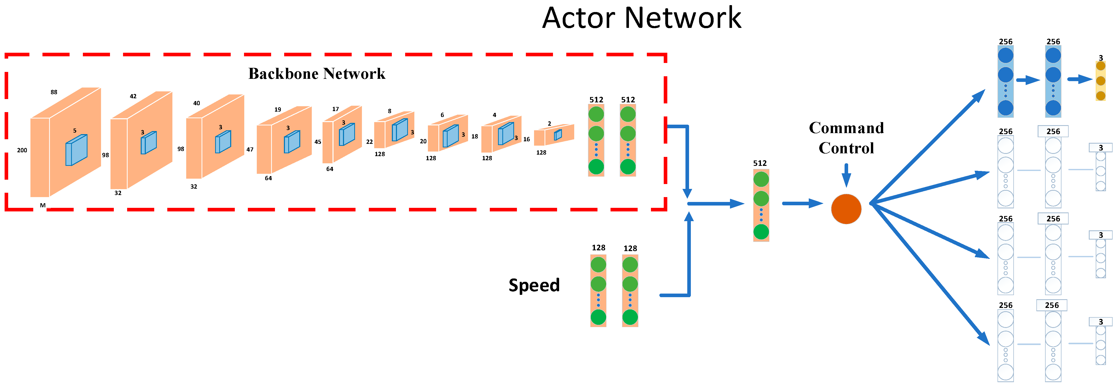
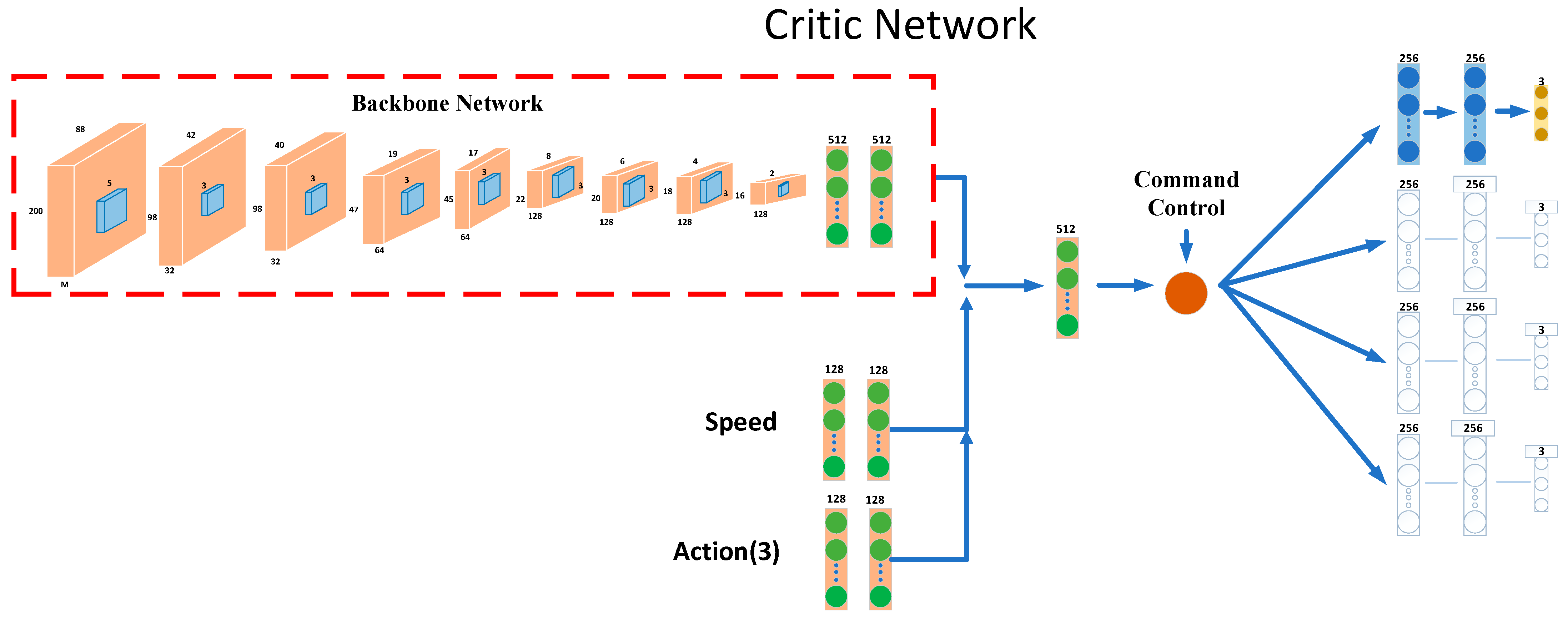
| Controllable Imitative Reinforcement Learning (CIRL) | The CIRL initializes the pre-trained model weights of the actor network through imitation learning. | CIRL also proposes adaptive strategies and steering angle reward functions for different control signals (i.e., following, straight ahead, right turn, left turn) to improve the model’s ability to handle varying situations. | CIRL does not perform image classification and image enhancement, and in practice, some false detections occur. |
| Serial No. | Control Volume | Type | Description |
|---|---|---|---|
| 1 | Speed | float | - |
| 2 | Steer | float | [−1.0, 1.0] |
| 3 | Throttle | float | [0.0, 1.0] |
| 4 | Brake | float | [0.0, 1.0] |
| 5 | High-level command | int | (2 Follow lane, 3 Left, 4 Right, 5 Straight) |
| Parameters | Value |
|---|---|
| Buffer size | 100,000 |
| Batch size | 32 |
| Discount factor | 0.99 |
| Learning rate of actor | 0.0001 |
| Learning rate of critic | 0.001 |
| Max steps per episode | 3000 |
| Total training episodes | 8000 |
| Optimizer | Adam |
| Train_PLAY_MODE = 0 | Train = 1 Test = 0 |
| τ | 0.001 |
| Town | Weather ID | Lane Departure | Driving in other Lanes | Crash | Hitting Someone |
|---|---|---|---|---|---|
| Town 1 | 1 | 16.74 | 14.13 | 16.74 | 16.74 |
| 2 | 11.58 | 12.05 | 13.26 | 13.26 | |
| Town 2 | 1 | 9.41 | 9.54 | 11.95 | 11.95 |
| 2 | 13.37 | 12.79 | 15.46 | 15.46 |
| Town | Weather ID | Lane Departure | Driving in other Lanes | Crash | Hitting Someone |
|---|---|---|---|---|---|
| Town 1 | 1 | 0 | 1.33 | 0 | 0 |
| 2 | 2.54 | 1.68 | 0 | 0 | |
| Town 2 | 1 | 3.01 | 2.86 | 0 | 0 |
| 2 | 3.47 | 4.20 | 0 | 0 |
| Town | Weather ID | Lane Departure | Driving in other Lanes | Crash | Static Collision |
|---|---|---|---|---|---|
| Town 1 | 1 | 21.09 | 20.21 | 22.58 | 22.58 |
| 2 | 22.26 | 21.54 | 26.71 | 26.71 | |
| Town 2 | 1 | 16.21 | 17.26 | 21.39 | 21.39 |
| 2 | 16.45 | 14.36 | 24.83 | 24.83 |
| Town | Weather ID | Lane Departure | Driving in other Lanes | Crash | Static Collision |
|---|---|---|---|---|---|
| Town 1 | 1 | 1.14 | 2.02 | 0 | 0 |
| 2 | 2.47 | 3.63 | 0 | 0 | |
| Town 2 | 1 | 4.33 | 4.67 | 0 | 0 |
| 2 | 6.68 | 6.97 | 0 | 0 |
| Town | Weather ID | Lane Departure | Driving in other Lanes | Crash | Hitting Someone |
|---|---|---|---|---|---|
| Town 1 | 1 | 22.91 | 20.27 | 23.69 | 21.54 |
| 2 | 19.95 | 17.71 | 19.81 | 20.23 | |
| Town 2 | 1 | 8.67 | 10.26 | 12.94 | 10.37 |
| 2 | 5.26 | 7.68 | 8.34 | 10.26 |
| Town | Weather ID | Lane Departure | Driving in other Lanes | Crash | Hitting Someone |
|---|---|---|---|---|---|
| Town 1 | 1 | 2.82 | 3.58 | 3.12 | 3.33 |
| 2 | 3.85 | 5.33 | 4.62 | 3.14 | |
| Town 2 | 1 | 11.0 | 9.34 | 7.67 | 6.41 |
| 2 | 12.18 | 13.68 | 10.73 | 9.13 |
Publisher’s Note: MDPI stays neutral with regard to jurisdictional claims in published maps and institutional affiliations. |
© 2022 by the authors. Licensee MDPI, Basel, Switzerland. This article is an open access article distributed under the terms and conditions of the Creative Commons Attribution (CC BY) license (https://creativecommons.org/licenses/by/4.0/).
Share and Cite
He, L.; Ou, J.; Ba, M.; Deng, G.; Yang, E. Imitative Reinforcement Learning Fusing Mask R-CNN Perception Algorithms. Appl. Sci. 2022, 12, 11821. https://doi.org/10.3390/app122211821
He L, Ou J, Ba M, Deng G, Yang E. Imitative Reinforcement Learning Fusing Mask R-CNN Perception Algorithms. Applied Sciences. 2022; 12(22):11821. https://doi.org/10.3390/app122211821
Chicago/Turabian StyleHe, Lei, Jian Ou, Mingyue Ba, Guohong Deng, and Echuan Yang. 2022. "Imitative Reinforcement Learning Fusing Mask R-CNN Perception Algorithms" Applied Sciences 12, no. 22: 11821. https://doi.org/10.3390/app122211821
APA StyleHe, L., Ou, J., Ba, M., Deng, G., & Yang, E. (2022). Imitative Reinforcement Learning Fusing Mask R-CNN Perception Algorithms. Applied Sciences, 12(22), 11821. https://doi.org/10.3390/app122211821