1. Introduction
This paper is an extended version of a paper published in the Contributions to International Conferences on Engineering Surveying, INGEO & SIG2020, Online Conference, Croatia, 22–23 October 2020 [
1].
Structural health monitoring (SHM) of engineering structures can, besides physical sensors (accelerometers, LVDT, encoders), be performed by geodetic instruments and is usually done by GNSS in combination with robotic total stations (RTS). GNSS offers great coverage and RTS offers high-precision measurements. Today, modern total stations come with different integrated sensors. With the integration of image sensors into total stations (TS), so-called image assisted total stations (IATS), and due to rapid technological development, the different sensor classes, each with their specific advantages, can be unified, utilized, and fused as one single (nearly) universal instrument [
2]. This integration offers wide coverage of different geodetic tasks to be resolved more quickly, easily, and more precisely in comparison with classical geodetic methods and instruments. It even offers possibilities to solve some tasks that were not possible in the past with the usage of classic TS. With an appropriate system calibration provided, these images and video frames are accurately geo-referenced at any time. They are particularly suitable for deformation monitoring of civil engineering structures, i.e., structural monitoring and geo-monitoring of hazardous areas, which are very hard to approach. Today, state-of-the-art IATS comes with a scanning function (image-assisted scanning total station—IASTS). Modern TS are multi-sensor systems which can determine the three-dimensional coordinates of target points by combining horizontal angle, vertical angle, and distance measurements [
3]. IATS have possible applications in semiautomated object reconstruction systems [
4], fully automated deformation monitoring systems [
5], industrial measurement systems [
6], measurements of vibration amplitudes by means of high-frequency image measurements [
7], and the capture of additional information such as high-frequency motions or intensity fluctuations of patterns using image sensor to derive the temperature gradient of the atmosphere as a decisive influence parameter for angular refraction effects and monitoring of cracks [
8,
9].
Leica MS60, Trimble SX12 and Topcon GTL-1000 combine imaging with scanning on a level that is not rudimentary, so we can call them image-assisted scanning total stations (IASTS). In [
10], Leica MS60, Trimble SX12, and Topcon GTL-1000 are compared with their main specifications and characteristics. All instruments have a scanning function, and they are classified as multi stations (MS), so-called IASTS. These three instruments, at the moment, represent the state-of-the-art geodetic instruments in the world. For the purpose of this study, we used Trimble SX10 predecessor of Trimble SX12.
All instruments and sensors have their own advantages and shortcomings. The biggest shortcomings of TS, RTS, IATS and GNSS is the fact that we can only monitor one discrete point at time. We cannot monitor the whole surface of the engineering structure. In some ways, IATS overcome this deficiency using image sensor and obtaining images of one part of the structure, but can still only measure displacements of multi points but parallel to the image sensor in two axes. So, new methodologies and instruments need to be developed [
11].
A fundamental change in geodetic deformation monitoring is currently taking place. Nowadays, areal measurements are increasingly used instead of pointwise observations (of manual selected discrete points) as done in the past. Frequently, laser scanners are used, as these allow a fast, high resolution and dense acquisition of 3D information. However, it is challenging to uncover displacements and deformations and changes in multi-temporal point clouds as no discrete points are measured, and only changes in line of sight (of non-signalized areas) can be clearly detected automatically as distance variations. Further, rigorous deformation analysis and tests of significance of the results are missing [
12,
13]. Tests in laboratory conditions of the latest generation of laser scanners have concluded that the laser scanner can be used to detect vertical displacement non-natural targets marked with photogrammetry markers with millimeter accuracy [
14]. Image analysis techniques, in contrast, are very sensible for identifying displacements in transverse direction. Hence, a combined acquisition and analysis of point cloud and image data complement each other very well [
15].
In a research study [
15,
16] a novel approach of fusing image and laser scan data from the same instrument, such as a MS, to create an RGB+D image was proposed. D channel represents the distance channel interpolated from the laser scanner data. Detection and matching of identical image features from RGB+D images gathered from different measurement epochs is a use case for computer vision algorithms. 3D coordinates of the detected features can easily be calculated using RGB+D images. Matched image features can be used as substitutes for classic discrete points in displacement monitoring tasks and rigorous geodetic deformation analysis with tests of significance. Comparatively, the lack of discrete points is the biggest drawback of using laser scanner data (3D point clouds) for displacement monitoring and deformation analysis.
The proposed methodology and all needed steps to create RGB+D images and their subsequent use were field-tested in this research. The research, i.e., this article, is organized in five sections. After the introduction in section two the used instrument Trimble multi station SX10 is presented with its basic characteristics and possibilities. Basic principle of fusion of laser scan and image data from multi stations, as well as deformation analysis using point clouds and matching algorithms for RGB+D data in displacement monitoring is explained in section two also. In section three, the experiment test procedure is elaborated upon in detail. The focus of the research is to determine the achievable precision of the method in field conditions. The testing aims to compare RGB+D detected displacement of a tested wooden beam to the control data, extracted from a numerical model of the beams, based on measurements by a linear variable differential transformer (LVDT) sensor, all presented in section three. The achieved results are shown in section four regarding the optimal algorithm used for image feature and matching identical points between different measurement epochs obtained from RGB+D data. Data comparison of obtained results regarding the numerical and measured displacements of the beam, i.e., the differences between them are also shown in section four. Our aim was to verify that fusion of laser scans and image data (RGB+D) is applicable for structural health monitoring of engineering structures. The gap in the current research is the lack of numerical testing and validation of the RGB+D method, which the authors have tried to fill in this paper. In the end in section five discussion and some conclusions are derived.
2. Materials and Methods
For the test material, wooden beams were chosen. Wood was selected because of its excellent elastic properties, and because it exhibits large displacements under a small load. Pressure was applied in incremental steps to the middle of the test beams with the purpose of causing displacements. MS Trimble SX10 was used to capture picture data and scan data of the test beams. The relative movement of the element was measured with one or more LVDT sensors.
2.1. RGB+D Data from Multi Stations
Combining all the sensors and functions of the MS provides a new opportunity for data acquisition in the field and the subsequent data processing. The fusion of data acquired from the integrated RGB (red, green and blue) image sensors and laser scanner data and its application for displacement monitoring, was proposed by A. Wagner [
16], and will be discussed and tested further in this paper.
2.1.1. Multi Sensor Total Stations
MS offers a unique advantage for the engineering surveyors by encompassing multiple measuring sensors in one instrument. It combines the measuring abilities of the classic total station equipped with robotic functionalities with built-in RGB sensors and a laser scanning function.
Total stations by themselves are multi-sensor systems that provide highly accurate angle and distance measurements to a signal, i.e., prism and, less precisely, prismless, to nearly any other surface by laser measurements. Further functions are tilt correction by 2-axis inclinometers, automatic target recognition and tracking by image sensors and drive. These instruments are called robotic total stations (RTS).
In recent years, all significant surveying manufacture equipment has started to offer RTS with the addition of at least one integrated image sensor. Its original function was to collect additional data about the measured points. In the literature, these types of total stations are called image assisted total stations (IATS). There are several different models of integration of image sensors into the RTS. Image sensors can be built into the telescope, onto the telescope and onto the eyepiece of the telescope of the RTS [
10]. The best integration is when a coaxial camera is built into the telescope, which then uses the optics and magnification of the telescope. The coaxial camera’s axis coincides with the telescope axis, and the camera center is the same as the instrument center. Using the telescope magnification results in a lower ground sampling distance (higher spatial resolution) of the image compared to the overview camera, albeit at a smaller field of view [
17]. Most manufacturers use a 5-megapixel Complementary Metal-Oxide-Semiconductor (CMOS) sensor in their total stations.
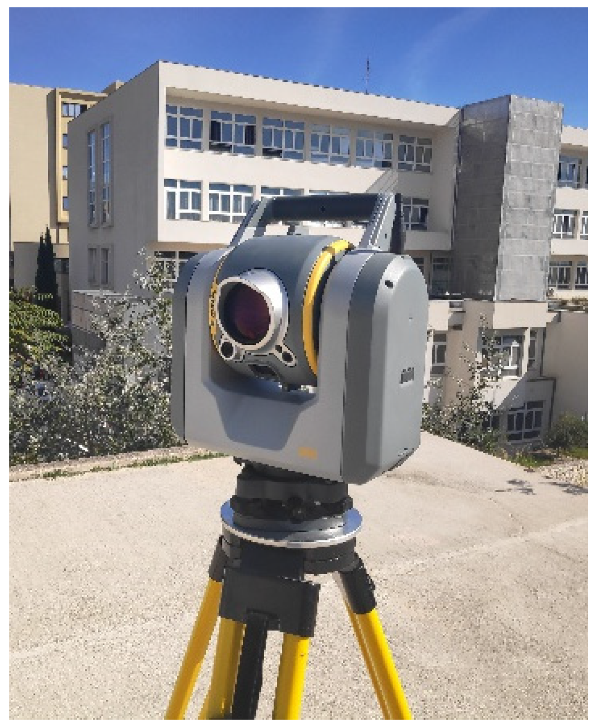
In addition to image sensors in the newer generations of IATS, manufacturers have started implementing laser scanner functions. The most significant disadvantage of the scanners integrated into total stations, when compared to terrestrial laser scanners (TLS), are their relatively slow rate of measuring data. Uniformly across all major manufactures, TLS measures data at a rate of around 1 MHz, while an integrated scanner usually measures data at a rate of 1 kHz, which results in long scanning times. The Trimble total station SX10, which is used for the testing by the author, as shown on
Figure 1, has pushed the limit of scanning rate up to 26.6 kHz [
18]. The relevant specification of the Trimble SX10 for the test is shown in
Table 1.
2.1.2. Fusion of Laser Scan and Image Data from Multi Stations
The resulting product from the fusion of laser scanner data an RGB image of the same scene is a generated RGB+D (Red, Green, and Blue + Distance) image. The D is the 4th channel of the image that depicts distance information from the laser scanner as pixel values.
It should be noted that the RGB+D images are also used in other fields of science, especially in applications of RGB+D cameras for computer 3D reconstruction of objects [
19].
This paper focuses on applying RGB+D images generated from MS precise measurements in displacement monitoring and deformation analysis.
The fusion of data from the laser scanner and camera data to RGB+D images combines the advantage of the two measuring methods. With laser scans and the resulting dense point clouds, distance changes in the line of sight can be easily detected. High-resolution image data, in contrast, are most sensitive to displacements perpendicular to the viewing direction of the camera [
15].
This process’s biggest hurdle is defining the precise spatial and angle relationship between the instrument, theodolite, and integrated camera. Empirical tests conducted with SX10 showed that methods like direct linear transformation (DLT) [
20] for determining camera offsets and parameters were not sufficiently precise for this use case. There is a high discrepancy between calculated parameters based on the test conditions, such as lighting, test target distance to the camera and measurement of 3D coordinates. For the DLT method, precise 3D coordinates of the photogrammetry targets are required. Precision for measuring 3D coordinates with the SX10 is around 2.5 mm, using prismless distance measurement [
18]. With all the problems mentioned, precise calculation of the camera and instrument parameters by the user is not ideal. The ideal solution is to obtain the technical specification of the used MS camera directly from the manufacturer. This solution was used for data processing in this paper.
2.2. Deformation Analysis Using Point Clouds
The emphasis in classic deformation analysis is on the discrete points which represent the object of interest. Deformation analysis compares the coordinates of the points, calculated from measurements in multiple epochs, to determine the possible displacements of the object with an appropriate statistical test of significance. Only a statistically verified result of a measurement may be used for further processing or interpretation. This is valid, in particular, for reliable alarm systems for the prevention of human and material damage [
17].
The goal of the RGB+D approach is to bypass the drawbacks of laser scanner measurement–point clouds by enhancing the data with corresponding RGB data, preferably captured with the same instrument, such as an MS, to identify corresponding (discrete) points between subsequent measuring epochs [
13]. The resulting data can then be integrated into a rigorous geodetic deformation analysis with a test of significance [
15].
Matching Algorithms for RGB+D Data in Displacement Monitoring
The biggest challenge of the RGB+D method used for displacement monitoring is how to identify corresponding (discrete) points between subsequent measuring epochs. Numerous matching algorithms have been developed for that purpose. The concept of feature detection and description refers to the process of identifying points in an image (interest points) that can be used to describe the image’s contents, such as edges, corners, ridges, and blobs [
21].
The most prominent and promising feature detection algorithms, applicable to RGB+D images in deformation analysis, are:
SIFT—Scale Invariant Feature Transformation [
22];
SURF—Speed Up Robust Features [
23];
BRISK—Binary Robust Invariant Scalable Keypoints [
24];
ORB—Oriented FAST and Rotated BRIEF [
25]
KAZE—Named after a Japanese word that means wind [
26].
All the algorithms mentioned are scale invariant, which enables them to match image features despite the scale change of an object between images (movement). David G. Lowe developed SIFT as a novel approach for image matching and feature detection. The basis of the algorithm is the transformation of image data into scale-invariant coordinates relative to the local features. An important aspect of the SIFT approach is that it generates a large number of features that densely cover the image over the full range of scales and locations [
22].
SURF approximates, or even outperforms, previously proposed image matching algorithms with respect to repeatability, distinctiveness, and robustness, yet can be computed and compared much more quickly [
23].
BRISK is proposed as an alternative image matching algorithm to SIFT and SURF, matching them in quality and with an emphasis on much less computation time [
24]. Because of the binary nature of the algorithms descriptors, image features can be matched very efficiently, which makes the algorithm applicable for real-time use.
ORB is a fast binary descriptor based on BRIEF (Binary robust independent elementary features [
27]) which is rotation invariant and resistant to noise. The contribution of ORB is the addition of a fast and accurate orientation component to FAST (features from accelerated segment test [
28]), the efficient computation of oriented BRIEF features, analysis of variance and correlation of oriented BRIEF features and a learning method for de-corelating BRIEF features under rotation invariance, leading to better performance in nearest-neighbor application [
25].
KAZE is a multiscale 2D feature detection and description algorithm in nonlinear scale spaces. Feature detection and description in nonlinear scale spaces. In contrast to previous approaches that rely on the Gaussian scale space, this method is based on nonlinear scale spaces using efficient AOS techniques and variable conductance diffusion. Despite of moderate increase in computational cost, the results reveal a step forward in performance both in detection and description against previous state-of-the-art methods such as SURF or SIFT [
26].
Algorithm selection will be predominantly scene (surveillance area) dependent because computation time is not a limiting factor for post-processing of data.
SURF, BRISK, ORB and KAZE have a direct implementation in MATLAB [
29].
MATLAB [
29] also has a built-in function “matchfeatures” for matching detected features between images. In this use case, images of the same test scene are taken in different epochs. There are multiple other software solutions available for matching features between images, and they all function on the same or similar mathematical principles. All performed tests in this research were coded and conducted in MATLAB.
Based on the test scene test results, algorithm selection will be discussed further in the data processing and results section of the paper.
3. Experimental Test Procedure
The general test procedure consisted of loading a test material element sequentially with pressure. The relative movement of the element was measured with one or more LVDT. Before every change of load was applied, a picture or multiple pictures in a panorama and a laser scan of the element was taken. Measured data were processed to create a fusion of a laser scan and image into RGB+D image for each load, i.e., epoch. From RGB+D images, displacements were calculated for detected matched points between the epochs. The resulting calculated displacement was then compared to the LVDT measured data.
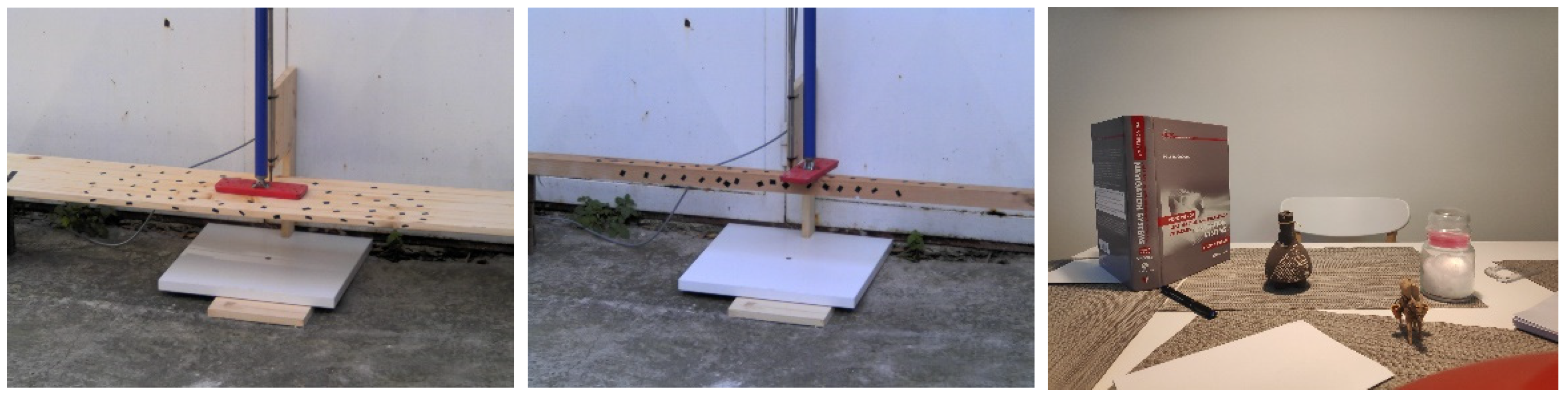
3.1. Testing Setup and Measurements
For the test material, wooden beams were chosen. Wood was selected because of its excellent elastic properties, and because it exhibits large displacements under a small load.
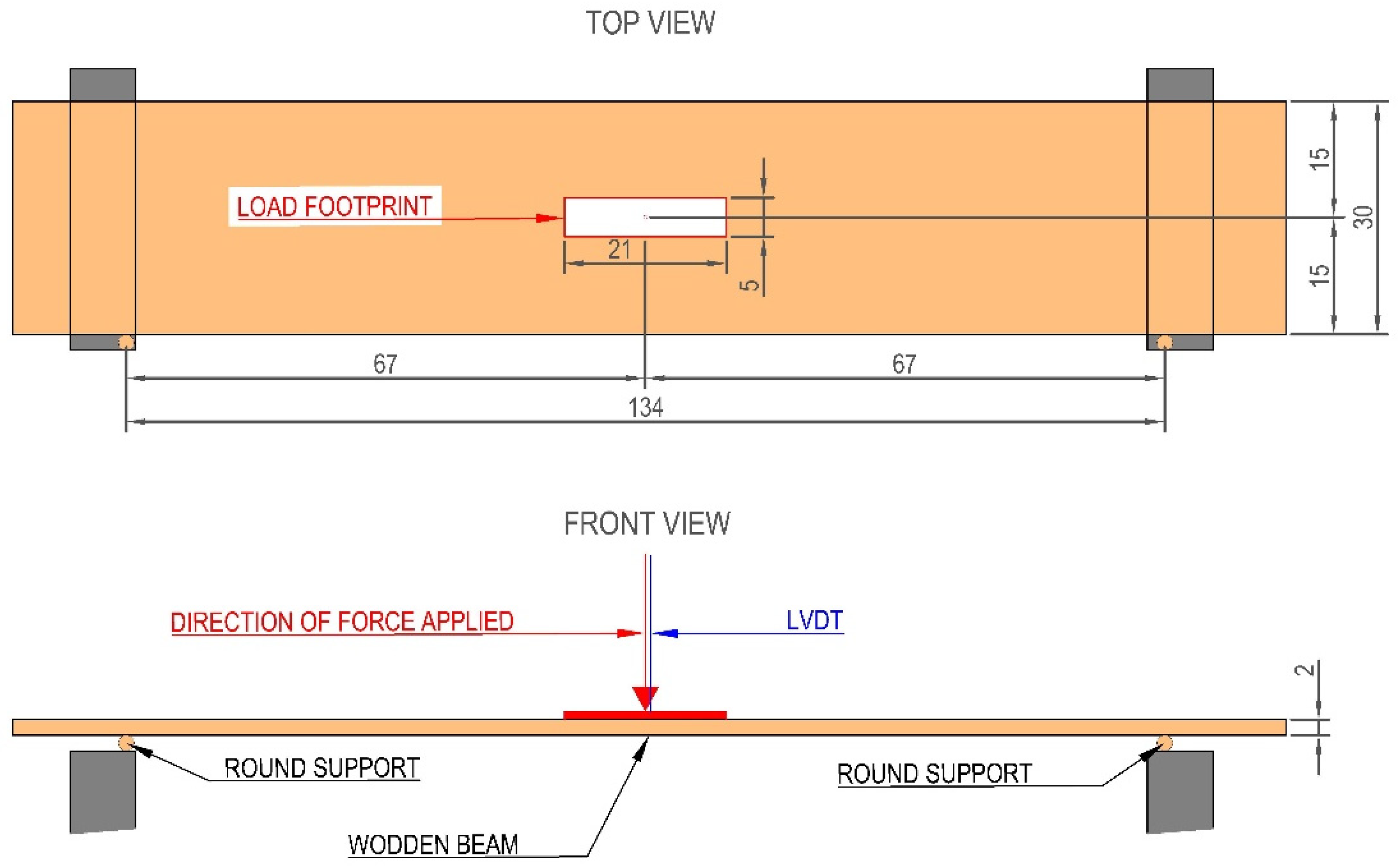
The wooden beam was supported on both sides, and the pressure was applied in the middle of the beam, as shown in schematic diagram in
Figure 2. The pressure distribution was not measured because it has no relevance for this type of test and subsequent calculations, but the overall force is known for every step of load increment using a small load cell integrated into the loading device. This setup was necessary to determine inputs for an independent numerical model of beam displacements. Small black shapes were added as additional targets on the wood beams to increase the number of detected features with the feature matching and detecting algorithms.
Displacements were measured with a LVDT, which is a common type of electromechanical transducer that can convert the linear motion of an object to which it is coupled mechanically into a corresponding electrical signal. LVDT typical sources of uncertainty are due to nonlinear electrical responses, mechanical positioning and orientation errors, electrical transmission noises, and digitalization errors. In the described measurement setup, the HBM WA100 LVDT sensor [
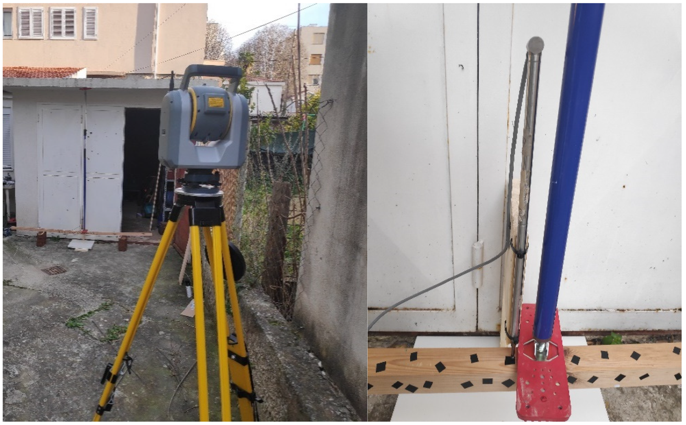
30] with a nominal measuring range of 0–100 mm was used. The used sensor’s nonlinearity is in the range of 0.2–1% of its entire measurement range. For reduced measuring range 0–20 mm used in this setup, overall accuracy is ±0.02 mm (obtained by previous laboratory calibration). The LVDT measuring accuracy is higher than the achievable accuracy of measurements obtained by Trimble SX10 by a factor of 100. The displacements obtained by LVDT were taken as a reference in this research for testing the accuracy of determined displacements from RGB+D images. LVDT was positioned in the middle of the beam where the pressure was applied to, as shown in
Figure 3 right.
MS instrument Trimble SX10 was used for the testing. The instrument was positioned roughly 5 m from the wood element, as shown on
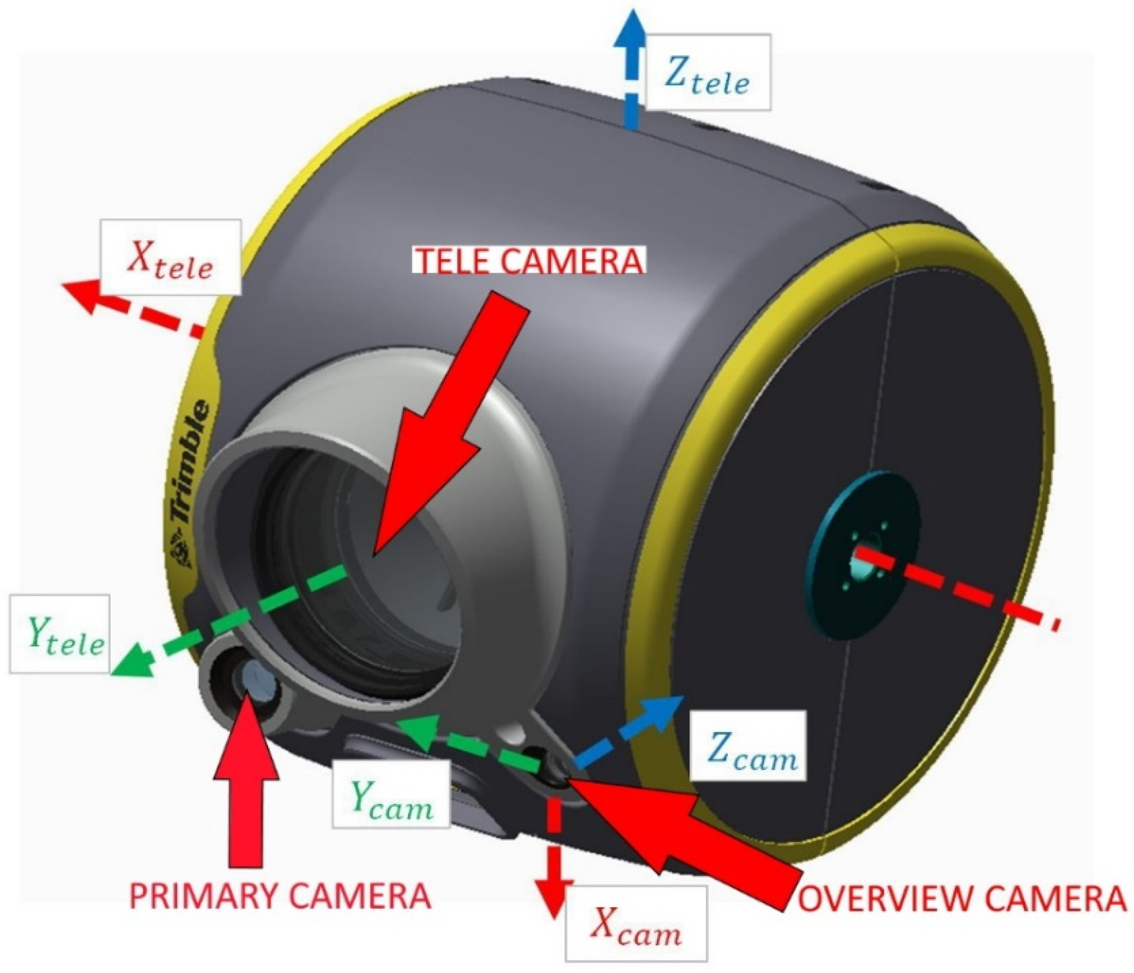
Figure 3 left. The distance was chosen based on the cameras field of view (FOV) so that the whole test field is visible within one image from the integrated primary camera. For the primary camera, the image size is 2592 × 1944 pixels, and at a 5 m distance, the ground sampling distance (GSD) is 0.3 mm. Location of the primary camera, in relation to the SX10 instrument body, is shown in
Figure 4.
The instrument station was set up in a local coordinate system. Control reference points were positioned around the test site and were used to check the stability of the instrument between the epochs.
The final test was conducted on two different wooden beams. For each element, four or five measuring epochs were conducted. Due to changing light conditions, only four measuring epochs were tested for the BEAM 1, in comparison to five for BEAM 2. The first and last epoch were without any pressure. For epochs two to five, rising pressures were applied so that different displacements were obtained and then measured with the MS and LVDT, as shown in
Table 2. In each epoch, a picture was taken with the MS primary camera. For each image theodolite angles (
Hz,
V) measured from the MS are stored. Using the stored theodolite angles and camera parameters, external orientation of the camera can be easily calculated. The test area was then scanned in the scanner’s FINE resolution mode, which resulted in a measurement density of 1 mm. Data from the LVDT were continuously logged and stored.
3.2. Data Processing
Obtained data from MS Trimble SX10 used for the processing were images, point clouds, and a job file. The job file contained all metadata for a single job in an SX10; in this case, metadata about the captured images were extracted. Data processing was done using MATLAB and the code developed by the authors. The code was used to compare the data from two different epochs. For each epoch, an image, corresponding point cloud, and image metadata were loaded.
Data processing consisted of fusing image and scan data into RGB+D images for each epoch. Using image matching algorithms (SURF, BRISK, ORB and KAZE), identical points on images from different epochs were identified. Displacements for matched identical points are then calculated. Based on LVDT measurements, the wooden beam is numerically modeled as a reference for testing calculated displacement from RGB+D.
3.3. RGB+D Fusion
Fusion of image and scan data was based on matching theodolite angles (Hz and V) of points in the point cloud to corresponding pixels on images.
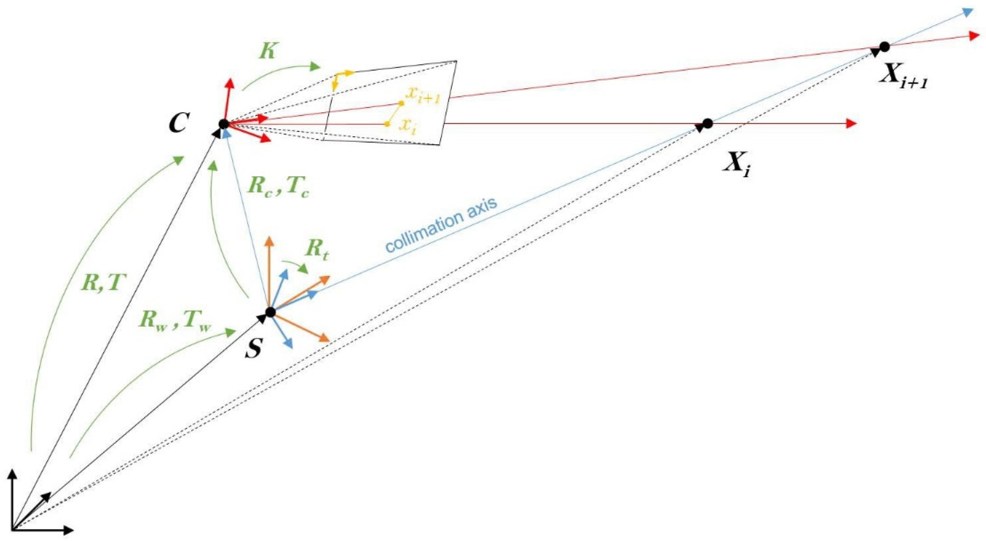
A shown in
Figure 5, the exterior orientation parameters of the camera R and T is a combination of three single transformations, the collimation axis is projected as a line into the image if an eccentricity between S and C exists [
17].
The steps necessary for image and scan fusion in this case are explained in the subsequent subchapters.
3.3.1. MS Instrument Setup
Standard geodetic procedure of instrument setup, like using resection to control points, is used for calculating the 3D coordinates of the instrument center (x, y and h) and determining the orientation of the instrument in the used coordinate system. Coordinate system can be absolute (world) and relative (local). For the purpose of testing a local coordinate system was used. This step calculates the transformation parameters from the absolute od relative coordinate system to the instrument coordinate system.
Based on the instrument setup data and horizontal and vertical limb measurements theodolite angles (Hz and V) can be calculated for each telescope position. This step calculates the transformation parameters from instrument coordinate system to the telescope coordinate system.
Trimble MS stores the data necessary to calculate the theodolite angles of the telescope for any measurement or an image in a Bivector format in the instrument job file [
31]. The exact formulas and algorithms used for calculating the theodolite angles cannot be show in this paper, as it is Trimble Geospatial proprietary code, and the authors were instructed not to distribute it further.
3.3.2. Image Data Processing
The described process in this subchapter is unique to the use of Trimble MS instrument. The process is repeatable using any other MS from other manufacturers, but it would involve more steps and calculations.
The camera is modeled as a pinhole camera with known intrinsic parameters from the manufacturer represented in a calibration matrix
K:
where
denotes the focal length and
the image coordinates of the principal point.
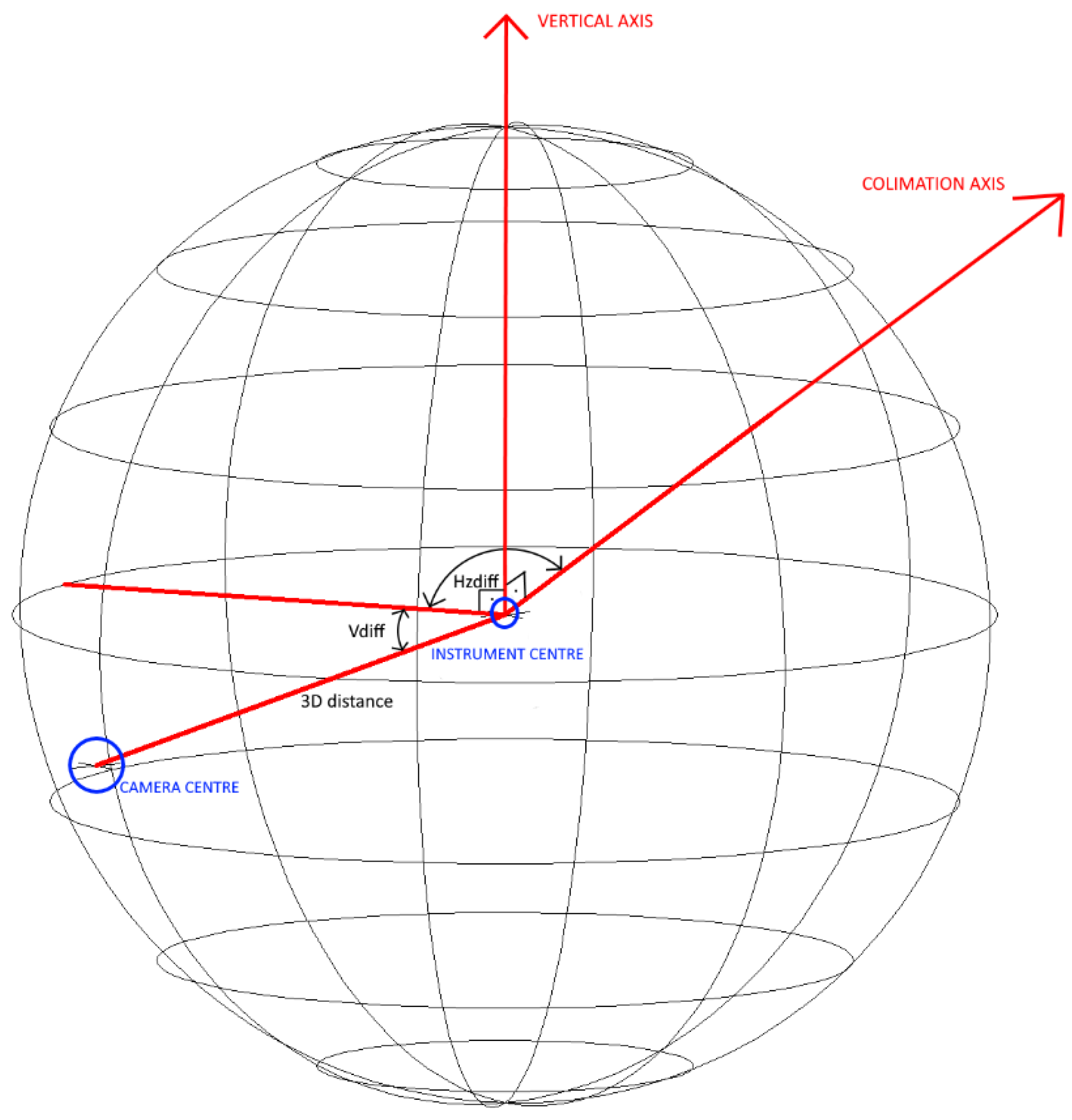
The coordinates of the camera center in the used coordinate system were calculated based on the telescope theodolite angles and the nominal offsets of the camera center from the instrument center. Nominal offsets values were known from the mechanical design blueprint of the instrument data, provided by the manufacturer. The mathematical model that defined the coordinates of the camera center based on the telescope theodolite angles was created. The camera center circled around the instrument center on a sphere, as depicted in
Figure 6. Angle differences between the collimation axis and vertical axis and the 3D distance were constants.
For the given telescope theodolite angles (
Hz and
V), camera center theodolite angles in the used coordinate system are defined as:
Coordinates of the camera center are defined as:
where
are the coordinates of the instrument center from the instrument setup.
Exterior orientation parameters of the camera are calculated based on a Bivector that defines the relation between the camera and telescope axis. Bivectors for each image are stored in the MS job file. Bivector from the camera to the telescope defines the 3D rotation of the camera around the theodolite axis as a combination of the general main rotation, collimation error, temperature dependent part, and any user calibration [
32]. The use of Bivectors replaces the standardly used transformation from 3D world coordinates into image pixel positions and backward transformation using rotation matrices and translation vectors. This step calculates the transformation parameters from the telescope coordinate system to the camera coordinate system. The exact formulas and algorithms used for calculating the extrinsic camera parameters cannot be shown in this paper, as it is Trimble Geospatial proprietary code, and the authors were instructed not to distribute it further.
The use of self-calibrated data from Bivector simplifies the calculation process and mathematical models, from the manual version, where users would need to calculate everything themselves. This step calculates the theodolite angles (Hz and V) of the camera principal point in the used coordinate system.
Within the Trimble MS job file, calibrated values of angle difference per pixel are stored for each image. Theodolite angles for each pixel can be defined in a simplified way as:
where
are the image coordinates of the principal point,
are the image coordinates of the pixel and
is calibrated value for pixel angle difference. Approximately
equals to 18.3″ for the primary camera of SX10. Because the image features are roughly on the same part in each image, effect of any residual camera calibration errors are negligible.
All image data is stored within a 5-dimensional matrix that have the same dimension as the base image. Each position in the matrix represents one image pixel, first three matrices contain RGB data for the pixel and the last two contain theodolite angles (Hz and V) of the pixel.
3.3.3. Point Cloud Processing
Product of laser scanning is a point cloud. For each point in the cloud 3D coordinate (x, y and h) are determined in the used coordinate system, defined by the instrument setup. The point cloud processing consists of calculating theodolite angles (Hz and V), 3D distances () and 2D distances () from the camera center to each point of the cloud based on the 3D coordinates of points and calculated coordinates of the camera center. 2D and 3D distances were calculated from 3D coordinates of matched points in different epochs using the formula for Euclidean distance between two points in Cartesian space.
Theodolite angles (
Hz and
V) of each point in point
i cloud are defined as:
where
and
are the coordinates of the camera center, in the defined coordinate system.
3.3.4. Image and Point Cloud Data Fusion
Data measured with the instrument, point cloud and measurements, are in the same coordinate system, defined through the instrument setup. Coordinates of the camera center and theodolite angles (
Hz and
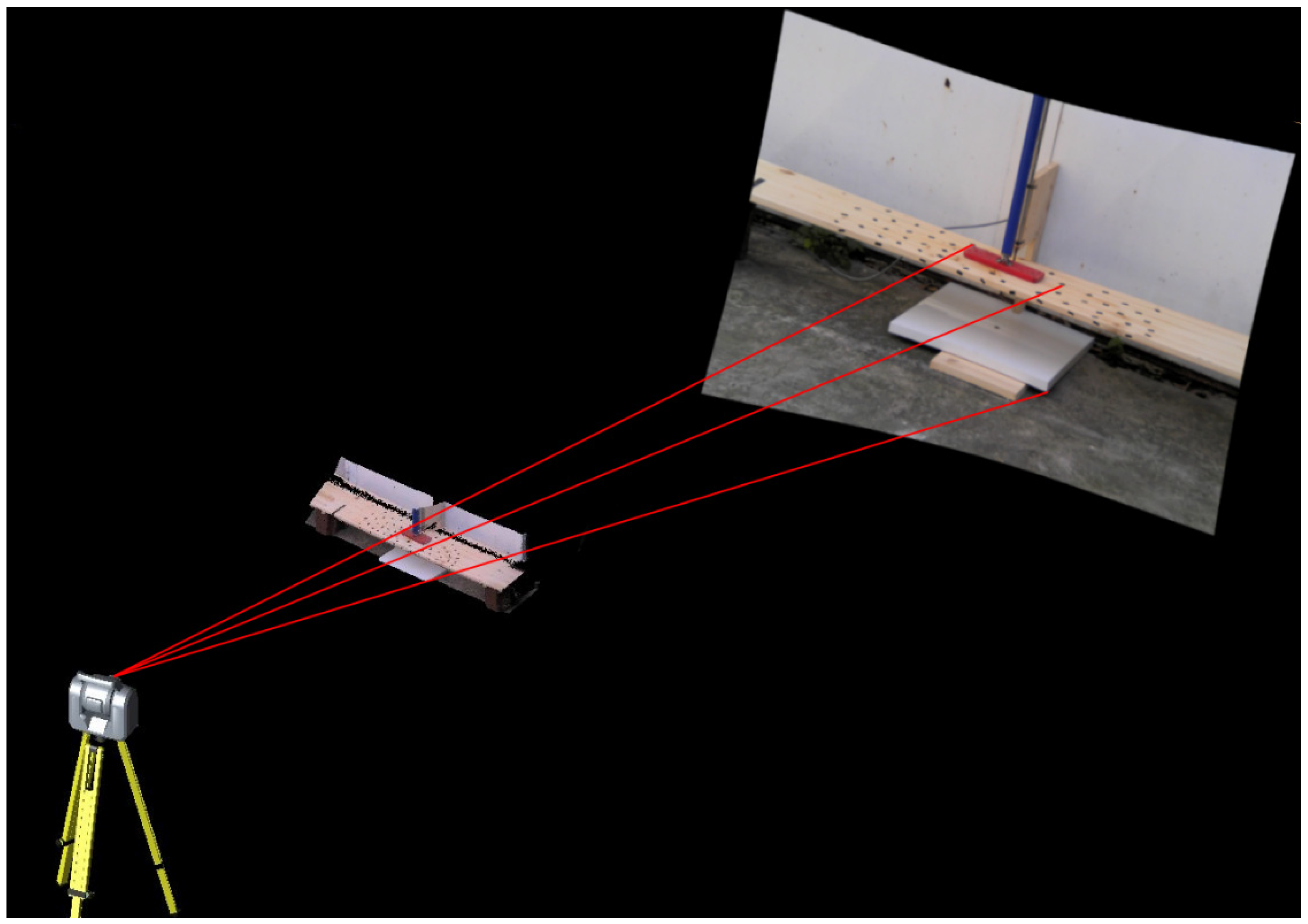
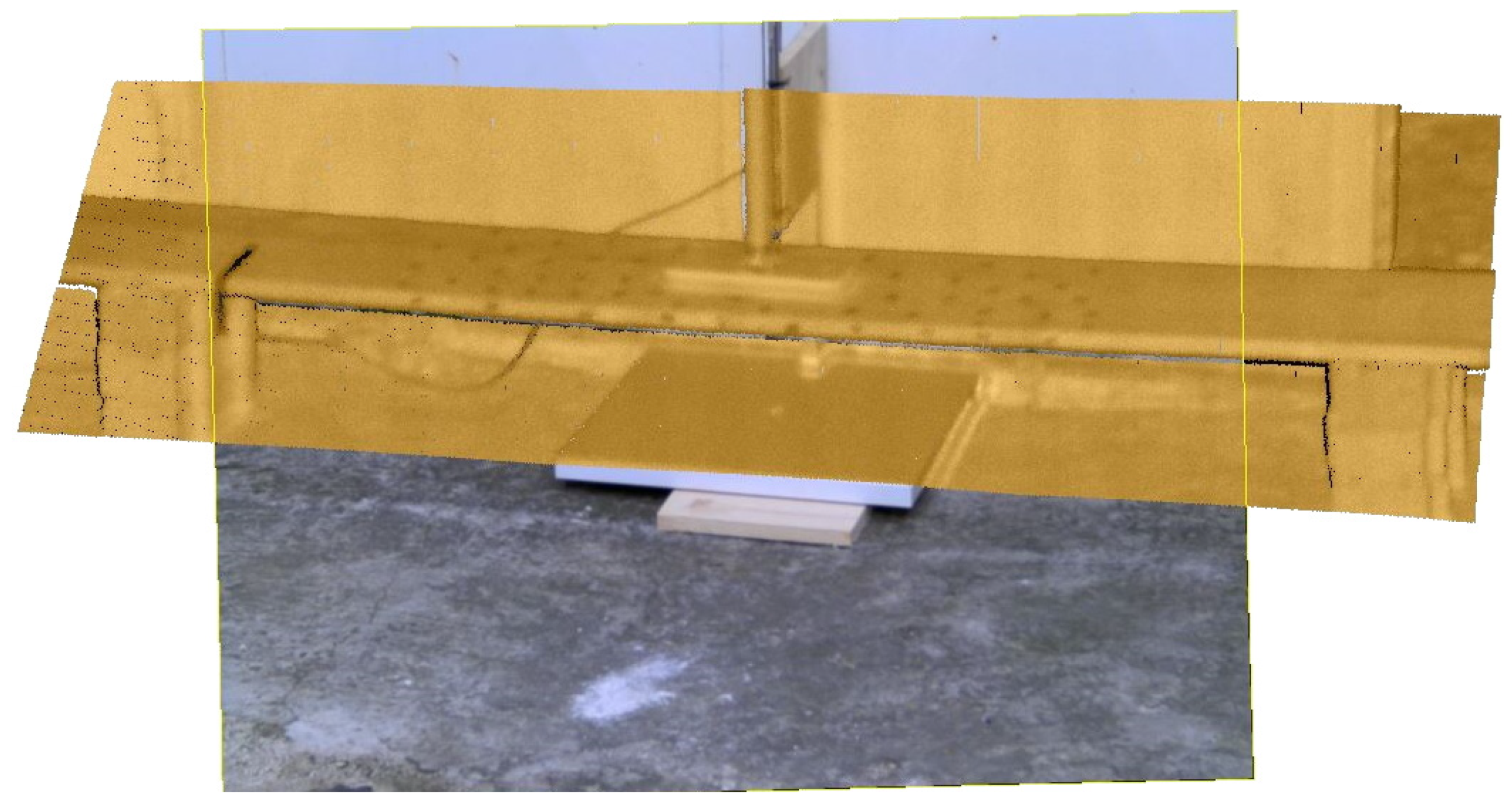
V) of each pixel are in the same coordinate system. Spatial rays projected from the camera center pass through the point cloud and the matching pixel in the image, as shown in
Figure 7. Rectified images of the test area overlap with the point cloud (highlighted yellow) of the same area, an example is shown in
Figure 8.
The next step is matching between the image and point cloud, based on minimal angle difference, to assign 3D distances to some of the pixels. The goal is to find a point from the point cloud that lays on the same spatial ray as a pixel in the image.
Pixel position for a point in the point cloud can be defined as:
where
is a matrix with horizontal theodolite angles for each pixel,
is a matrix with vertical theodolite angles for each pixel. The function min in Matlab return se matrix index (row and column) of the minimum value in the matrix. The result are the pixel positions in image of each point in the point cloud.
Based on the pixels with distance values, an external boundary of the scan data is created for the image, Region Of Interest (ROI). The boundary is used to prevent the interpolation of data to the pixels of the image that are not covered by any point cloud data.
Because the number of pixels in the image is usually larger than the number of point cloud points, 3D distances for the empty pixels are calculated using a 2D interpolation algorithm [
33].
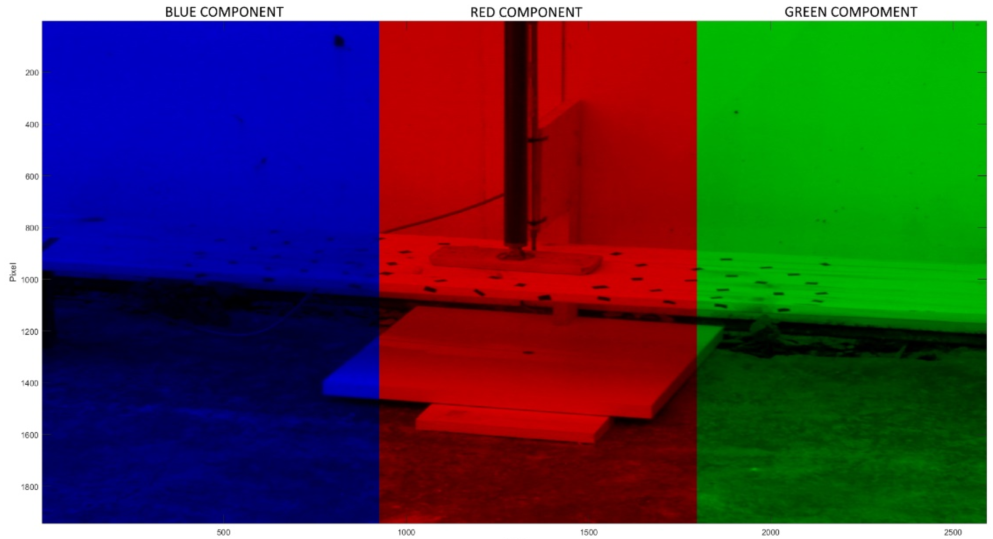
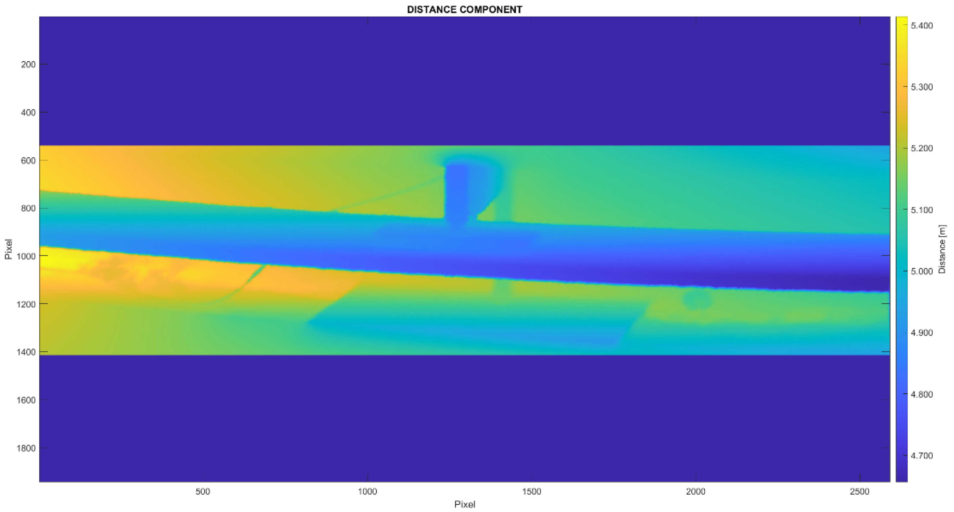
The result of this step is an RGB+D image for each epoch. For each image pixel, RGB values, as shown in
Figure 9,
Hz and
V angles, and 3D distance are known, as shown in
Figure 10; also, the image’s ROI is defined. The data were stored within a 6-dimension matrix, where in addition to the aforementioned five matrices, the sixth matrix contained the distance data for each pixel.
3.4. Image Matching
Image-matching algorithms are used to detect identical points features between RGB+D images from different epochs. The results of image matching are the pixel location of matched identical points in two images from different epochs. As stated before, multiple algorithms are applicable for this use case. To determine the optimal algorithm for this use case, empirical tests were conducted with different image datasets.
Matching algorithms SURF, BRISK, ORB, and KAZE were used and tested as they have a direct implementation in MATLAB. All of the test results of matching were also filtered for outliers. In this test case, filtering was done based on the calculated projective transformation between the images and measured maximum displacements from LVDT.
The first test consisted of testing the algorithms with all combinations of images in a dataset. Test parameters will be the average number of features in images, the number of matched features between images with and without outlier removal, processing time and normalized time for two images and matching between them, and maximum RAM usage of the algorithm.
The second test consisted of testing the matching points from between epoch located on the top of the beam within the ROI. Points were selected manually to match the area of the wooden beam that was modeled as a reference. The test compared the number of used points in ROI and statistical parameters of the calculated residuals. The residuals were differences between height displacements calculated from the control data and measurements of RGB+D data.
Results of both tests of image matching algorithms will be further discussed in the results section, and they will be used as criteria for algorithm selection for the data processing.
3.5. Displacement Calculation
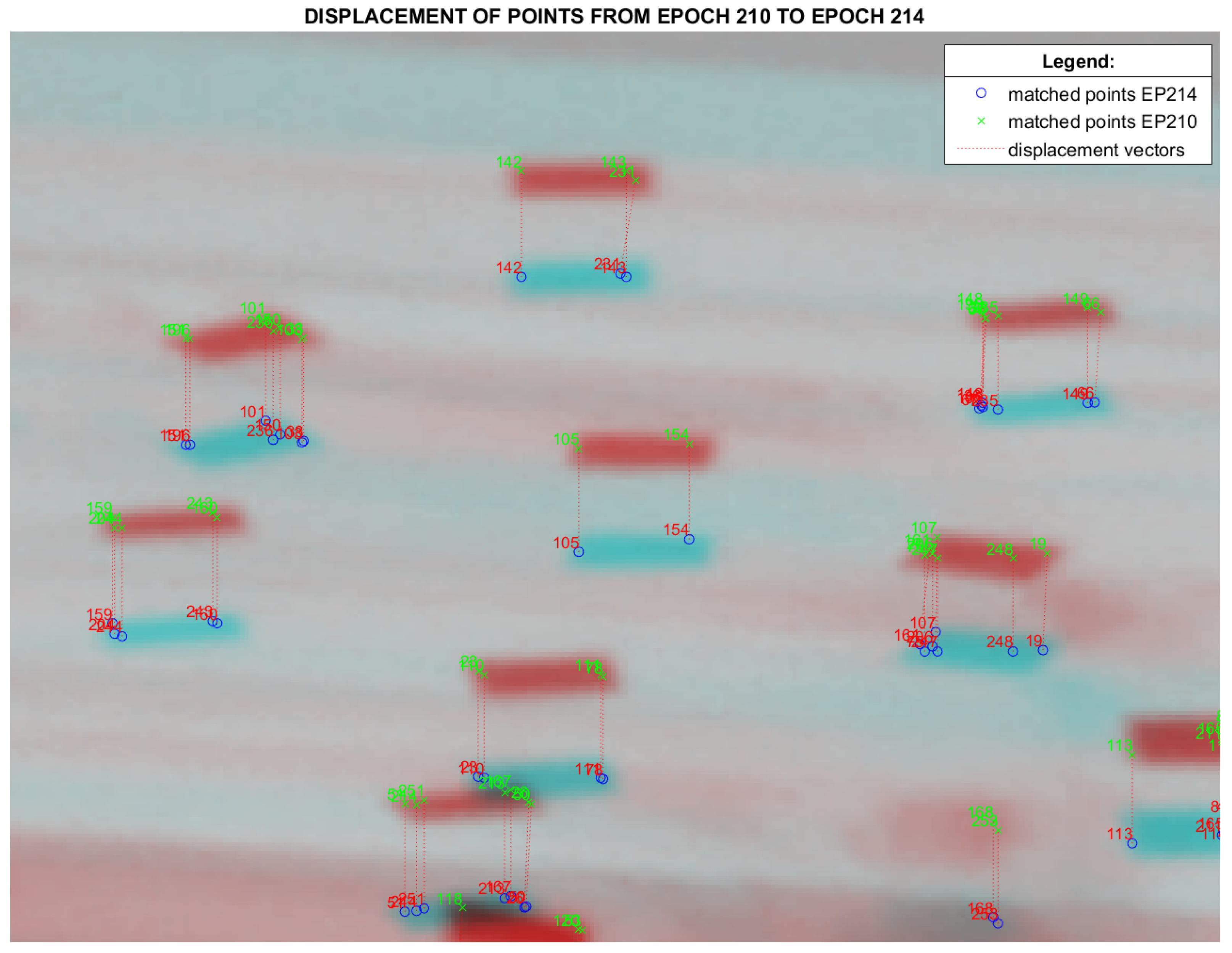
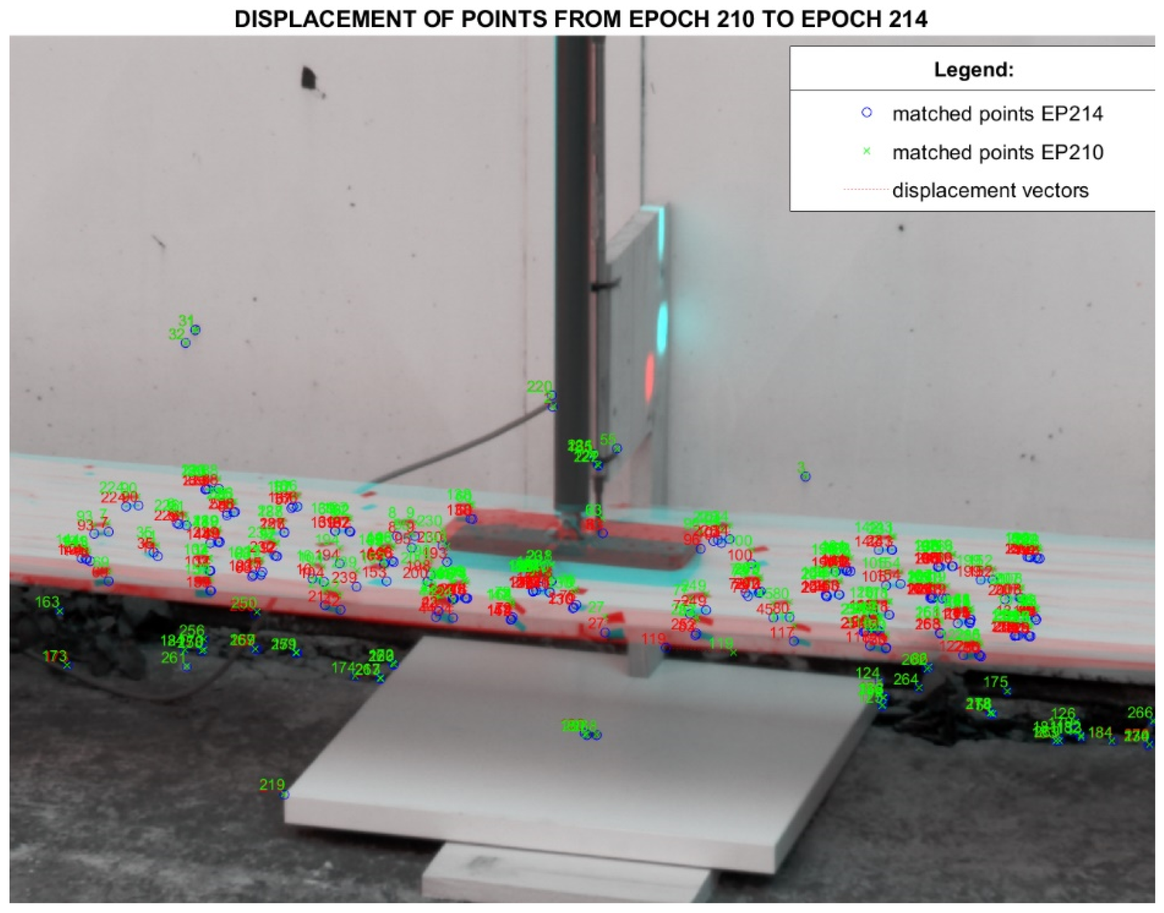
The outputs of image matching are identical feature pixels between two images, as shown in example in
Figure 11 and
Figure 12. Each image represents one measurement epoch. Based on the RGB+D data, 3D coordinates of each pixel in each image can be calculated. As stated before, for each image pixel in the ROI theodolite angles (
Hz and
V) and 3D distance
can be known.
3D coordinates of a pixel are defined as:
where
are the 3D coordinates of the camera centre, and
is defined as:
2D and 3D displacements of matched features can be calculated based on the calculated 3D coordinates of pixels in images from different measurement epochs. 2D and 3D distances were calculated from 3D coordinates of matched points in different epochs using the formula for Euclidean distance between two points in Cartesian space.
Displacements were calculated between four epochs for BEAM 1, and five epochs for BEAM 2. The wooden beams are shown later in the paper in
Section 4.1.
3.6. Creation of a Numerical Model Used for Control Data
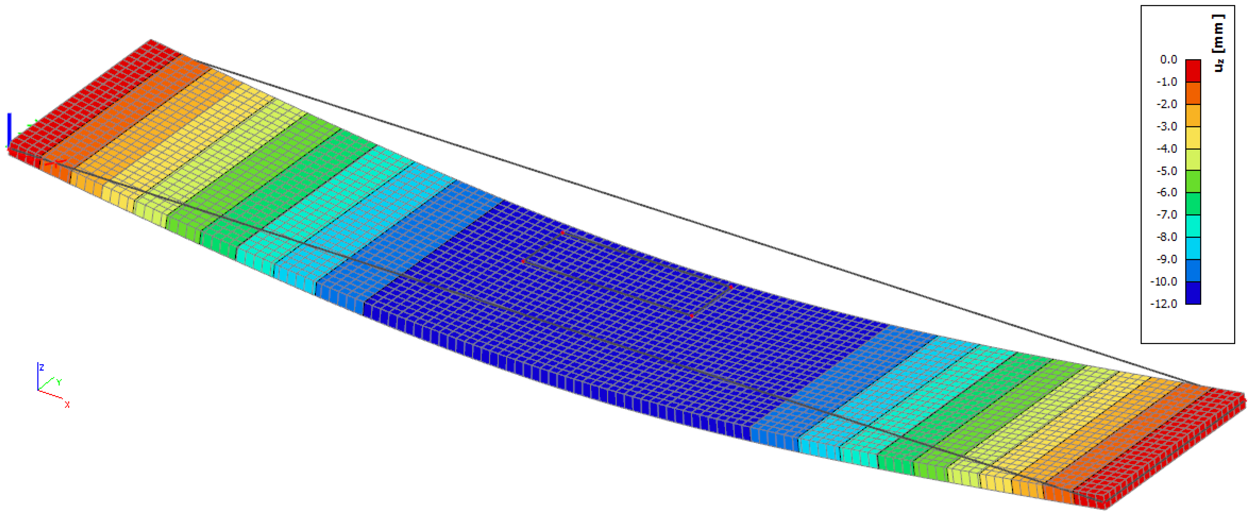
Based on the measurement and geometry data for the beam, measured on the test site and extracted from the point cloud and LVDT measurement data, a numerical model of the beam was created. The used numerical model was modeled in commercially available software SCIA Engineer 19.2 based on a finite elements method (FEM) structural analysis, which is the standard in civil engineering [
34]. The inputs for the model were the dimension and orientation of the wooden beam, mechanical properties of the timber material, and load. The material was timber class C14 (EN 338), with a modulus of elasticity of 7000 MPa and a shear modulus of 440 MPa. The load was applied to an area 200 × 70 mm in the middle of the top surface. The ultimate load was 16.9 kN/m
2. The load was deduced by comparing the maximum displacement of the model and was obtained from LVDT measurement. This approach accurately defined the material model instead of the general normative timber model. While performing numerical analysis, anisotropic properties of timber were not taken into account since displacements are due to bending, and along-grain stresses were dominant. The outputs of the model are displacements of points on the beams and internal forces, which were not used within the scope of this paper. Based on the numerical model, z-axis displacement (change of height) were calculated for every point on the beam in each epoch, as shown for epoch 214 displacement in
Figure 13. It should be noted that the test beams were not perfectly horizontal in space; also, the wooden supports were not perfectly horizontal and perpendicular to the beams. All the imperfections in the setup were accounted for and inputted in the model for calculations of displacements based on point cloud data. Coordinates of the numerical model were in the same coordinate system, which was defined by the instrument setup.
4. Results
The image matching algorithm comparison results will be shown, and the results will be used for selecting the optimal algorithm to use in this use case scenario.
The final output of the RGB+D data processing are the 3D coordinates of the matched points in both epochs. Based on the coordinates, 2D and 3D displacements can be calculated. Data were processed for all five measuring epochs for each wooden beam.
Calculated height displacement from RGB+D was compared to the control height displacement from the model based on the LVDT measurements. Differences between the two different height displacements were calculated as residuals. Statistical parameters of the residuals were used to discuss the validity and achievable precision of the RGB+D method.
4.1. Image Feature and Matching Algorithms
The first test consisted of testing the algorithms with all combinations of images for both test setups and image data set with images larger in size; test images are shown in
Figure 14. Tested parameters were the average number of features on images, the number of matched features between images with and without outlier removal, processing time and normalized time for two images and matching between them, and maximum RAM usage of the algorithm. The results provided a good starting reference for algorithm selection and showed the potential benefits and limits of the algorithms, as shown in
Table 3. KAZE and ORB algorithms were unable to complete the task on larger image datasets, with default settings, due to the lack of memory (the test computer had 16 GB of RAM) and had to be limited manually to a max of 55,000 features per image. The number of detected features and matched features varied greatly between algorithms. Normalized times for each test image dataset were used to compare the times objectively because the time of processing is dependent on the test computer configuration. Similar tests of the same algorithms done by other researchers [
35] showed different results, further stating that the algorithm selection is mostly test scene dependent.
The second test consisted of testing the matching points from between epoch that are located on the top of the beam, within the ROI. Points were selected manually to match the area of the wooden beam that is modeled as a reference. The test compared the number of used points in ROI and statistical parameters of the calculated residuals, as shown in
Table 4. Normalized time was calculated for each test image by dividing all the duration times with the longest duration. Normalized time provides a simpler and more intuitive way of comparing duration than comparing times in seconds.
Calculated statistical parameters of displacement showed no statistically significant difference. For significance testing, a two-sample t-test was used with a 5% significance level.
A comparison of the test results from the first and second test showed that the number of features does not correlate directly with the number of usable features for RGB+D. Based on the test results shown in
Table 3 and
Table 4, the ORB algorithm was shown to be the optimal algorithm for this test case, with good computing performance, the lowest processing times and the highest number of usable features detected in the ROI, and was used for image matching and sequential displacement calculation for the test scenes.
4.2. Control Data
As stated before, a numerical model of the test wooden beam for each epoch was created using LVDT measurements, point cloud data, and known geometry of the beams. The numerical model was based on the finite element method. Because point cloud data was used in the model, there was a high correlation (around 90 percent) between model data and measurement data. LVDT data were used in the model creation and as an absolute control of the modeled data.
4.3. Data Comparison
Height displacement from RGB+D and the control data were calculated between four epochs for BEAM 1. and five epochs for BEAM 2.
Matching points from each epoch were filtered manually and only the ones that were located on the top of the beam were used. Epochs were named based on the image file name to avoid confusion data in processing. The difference of the height displacements from the points and the model (residuals) as a reference were calculated. Statistical parameters for residuals for BEAM 1 are shown in
Table 5 and for BEAM 2 in
Table 6.
Standard deviation of
N scalar residuals
R was defined as:
where
μ is the mean of
R:
Standard deviation error is defined as:
Standard deviation error is used for quantifying the uncertainty around an estimate of the mean.
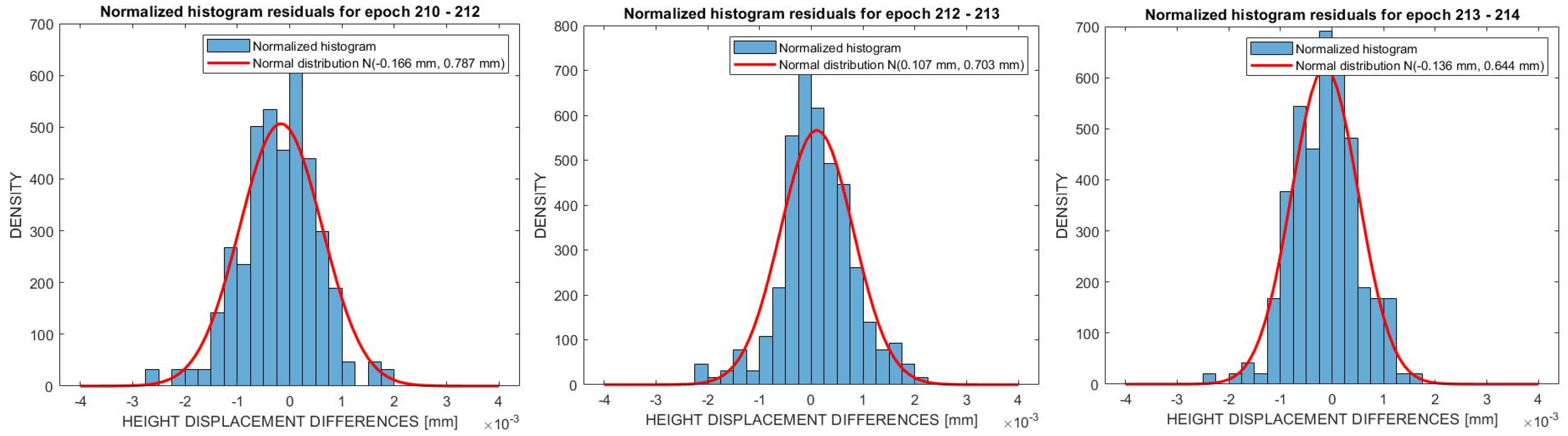
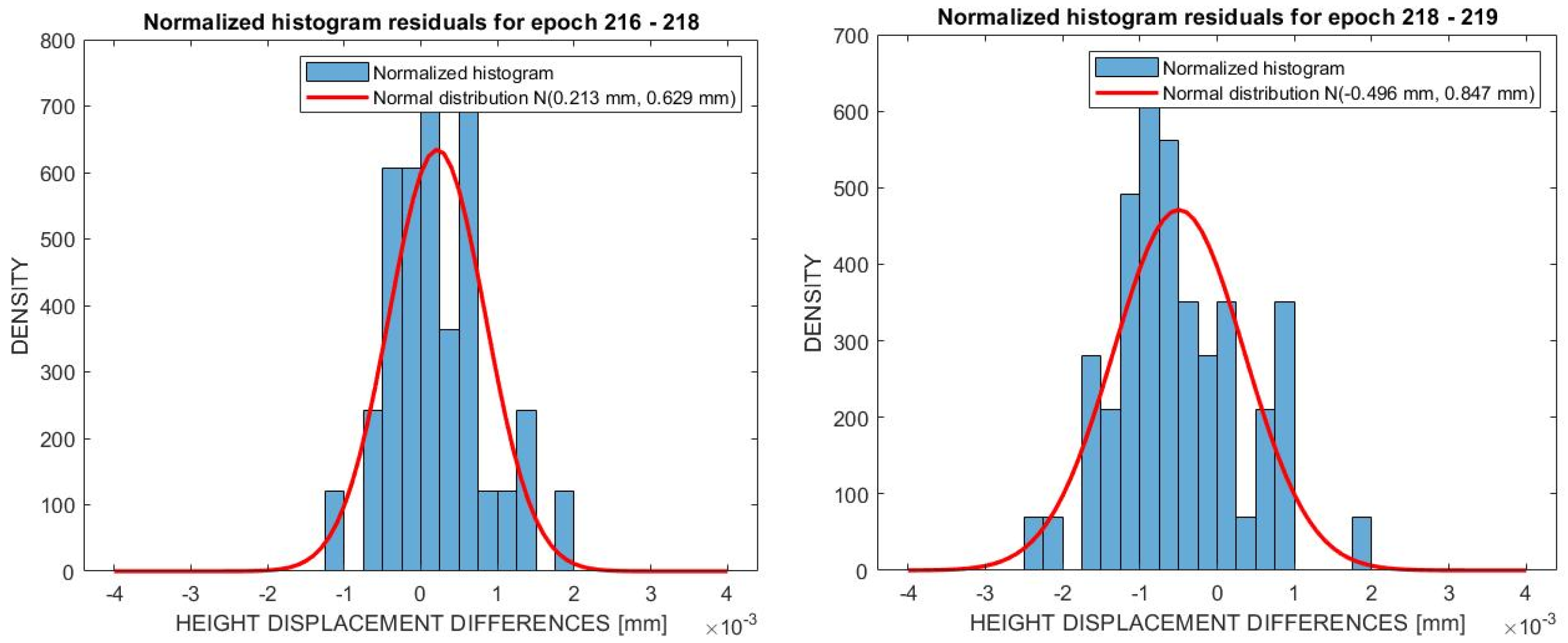
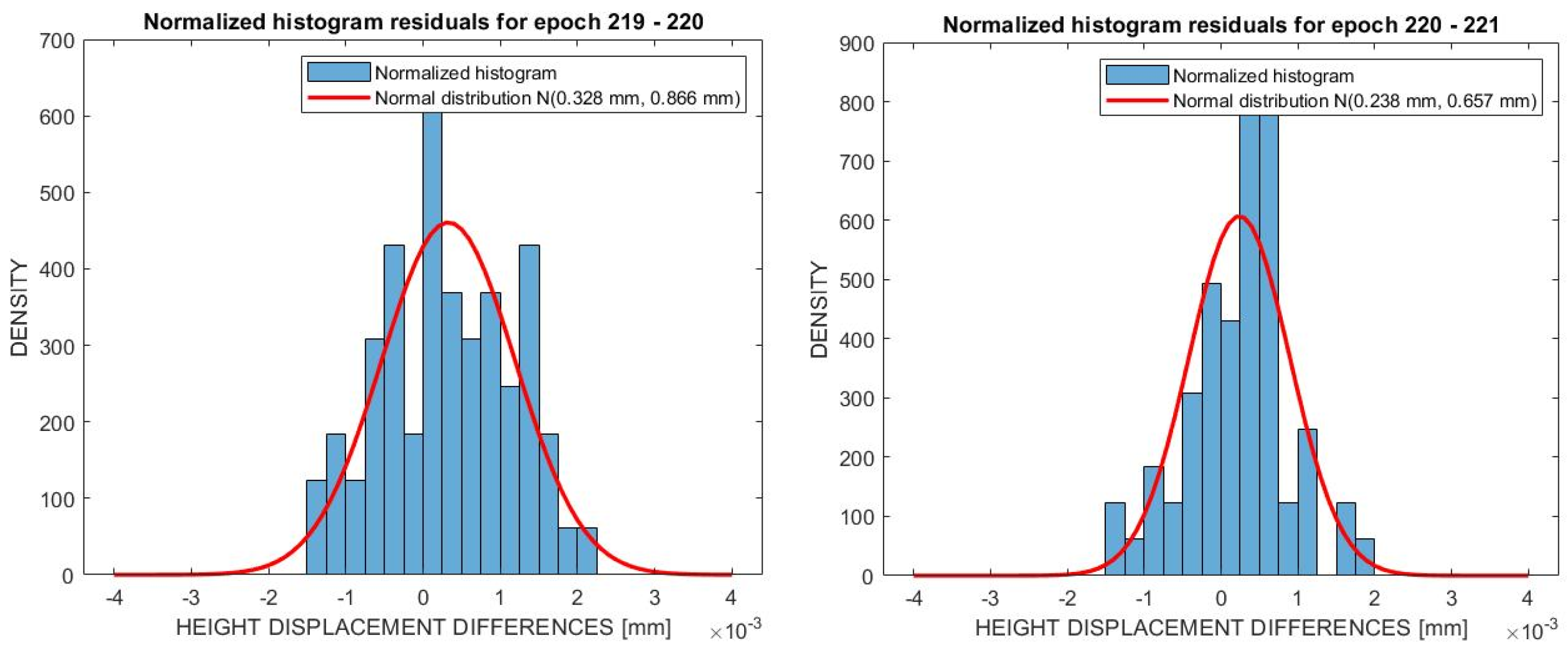
Distributions were fitted to residuals using the maximum likelihood method, with a significance level of 95%. The residuals were distributed normally with some outlier elements, as shown in
Figure 15 and
Figure 16.
Based on residual data, it was calculated that the precision of the image matching and fusion part of the RGB+D is ±1 mm, for this test case, with a GSD of 0.3 mm. Achievable precision of the RGB+D method was then calculated as a square root of the sum of squares of the standard deviation of 3D point measurement of Trimble SX10 [
18] and determined RGB+D. The calculated achievable precision for determining height displacement is ±2.7 mm.
5. Discussion and Conclusions
A. Wagner, in his research [
15,
17] proposed a methodology of fusing image and laser scan data from the same instrument, such as a MS, to create an RGB+D image and use the data for displacement monitoring.
Using computer vision algorithms such as SURF, BRISK, ORB and KAZE, distinct features of an image can be detected and tracked through different measurement epochs. Subsequently, their 3D coordinates can be determined from RGB+D images. This acts as a substitute for discrete geodetic points for further classic deformation analysis.
The proposed methodology was objectively and numerically tested within the scope of this research. The authors of this paper have developed a computer code, used for data processing, independently of the original author’s code to test the methodology’s validity objectively and numerically. After the methodology was validated by implementing the code on test data measured with a Trimble SX10 MS, the next step was to test the achievable precision numerically.
Tests of different image matching algorithms showed that algorithm selection is highly scene dependent. Based on test results, ORB algorithm was shown to be the optimal algorithm for this test case, with good computing performance, the lowest processing times and the highest number of usable features detected in the ROI. ORB was implemented in the final code, as the most optimal algorithm for this use case.
Reference data for testing the height displacements calculated from RGB+D were from a numerical model of the beam, modeled based on LVDT measurements, beam geometry, and point cloud data. Model data was built, to a degree, using the point cloud data, which made the model partially dependent on the data. Point cloud data were used for precisely determining the spatial position and orientation of the test beams, which is needed for the model to be in the same local coordinate system as the SX10. Because of the correlation of the model data with the point cloud data, model data can only be used to determine the precision of the image matching and fusion part of the RGB+D method. Due to correlation, model data cannot be used to determine the absolute accuracy of the RGB+D method.
The residuals (differences between RGB+D height and reference height obtained by LVDT) were distributed normally with some outlier elements, as shown in
Figure 15 and
Figure 16. suggesting that there was a negligible influence of systematic errors in the measurements and that the dominant factor was noise. Standard deviations for both epochs were below 1 mm with standard deviation error below 0.1 mm, as shown in
Table 5 and
Table 6. From the shown data, it can be concluded that the precision of the image matching and fusion part of the RGB+D is ±1 mm, for this test case, with a GSD of 0.3 mm. The calculated achievable precision for determining height displacement is ±2.7 mm.
Conducted tests and achieved results show the applicability of the RGB+D method for SHM using geodetic instruments such as multi stations. RGB+D method provides the ability to track multiple discrete points on the testing element through the testing, that only point clouds and relative measurement methods cannot provide. Thus, providing new data for testing the validity of behavior numerical models of an element being tested.
Based on the positive outcomes of conducted tests, further research in the real-world conditions on man-made structures is needed to prove the validity of RGB+D for the purpose of SHM. Further tests are planned to determine the relation between the GSD and achievable accuracy and precision.
Author Contributions
Conceptualization, J.P. and R.P.; methodology, J.P., R.P. and V.D.; software, J.P. and V.D.; validation, R.P. and B.K.; formal analysis, J.P. and V.D.; investigation, J.P. and V.D.; resources, J.P. and V.D.; data curation, J.P. and V.D.; writing—original draft preparation, J.P.; writing—review and editing, J.P., V.D., R.P. and B.K.; visualization, J.P. and V.D.; supervision, R.P. and B.K. All authors have read and agreed to the published version of the manuscript.
Funding
This research is partially supported through project KK.01.1.1.02.0027, a project co-financed by the Croatian Government and the European Union through the European Regional Development Fund-the Competitiveness and Cohesion Operational Programme.
Data Availability Statement
The data presented in this study are available on request from the corresponding author.
Acknowledgments
We would like to thank Geoprojekt d.d. Split, for lending us the Trimble SX10 for testing and Trimble employees C. Jorawsky and C. Grasse for their help with the technical specifications of the Trimble SX10.
Conflicts of Interest
The authors declare no conflict of interest.
References
- Peroš, J.; Paar, R.; Divić, V. Application of Fused Laser Scans and Image Data-RGB+D for Displacement Monitoring. In Contributions to International Conferences on Engineering Surveying; Springer: Cham, Germany, 2021; pp. 157–168. [Google Scholar]
- Wunderlich, T.; Wasmeier, P.; Wagner, A. Auf Dem Weg Zum Geodätischen Universalinstrument-Wie Nahe Am Ziel Sind IATS Und MS50? In Proceedings of the Terrestrisches Laserscanning 2014 (TLS 2014), Fulda, Germany, 11–12 December 2014; pp. 177–192. [Google Scholar]
- Lienhart, W.; Ehrhart, M.; Grick, M. High Frequent Total Station Measurements for the Monitoring of Bridge Vibrations. J. Appl. Geod. 2017, 11, 1–8. [Google Scholar] [CrossRef]
- Walser, B.H. Development and Calibration of an Image Assisted Total Station. Ph.D. Thesis, ETH Zurich, Zurich, Switzerland, 2004. [Google Scholar]
- Alexander, R.; Lehmann, M.; Kahmen, H.; Paar, G.; Miljanovic, M.; Ali, H.; Egly, U.; Eiter, T. A 3D Optical Deformation Measurement System Supported by Knowledge-Based and Learning Techniques. J. Appl. Geod. 2009, 3, 1–13. [Google Scholar] [CrossRef]
- Knoblach, S.E. Kalibrierung Und Erprobung Eines Kameraunterstützten Hängetachymeters. Ph.D. Thesis, Technische Universität Dresden, Dresden, Germany, 2009. [Google Scholar]
- Wasmeier, P. Grundlagen Der Deformationsbestimmung Mit Messdaten Bildgebender Tachymeter. Ph.D. Thesis, Technische Universität München, München, Germany, 2009. [Google Scholar]
- Huep, W. Scannen Mit Der Trimble VX Spatial Station. ZFV-Z. Fur Geodasie Geoinf. Und Landmanag. 2010, 135, 330–336. [Google Scholar]
- Reiterer, A.; Wagner, A. System Considerations of an Image Assisted Total Station-Evaluation and Assessment. AVN Allg. Vermess. Nachr. 2012, 119, 83–94. [Google Scholar]
- Paar, R.; Roić, M.; Marendić, A.; Miletić, S. Technological Development and Application of Photo and Video Theodolites. Appl. Sci. 2021, 11, 3893. [Google Scholar] [CrossRef]
- Paar, R.; Marendić, A.; Jakopec, I.; Grgac, I. Vibration Monitoring of Civil Engineering Structures Using Contactless Vision-Based Low-Cost IATS Prototype. Sensors 2021, 21, 7952. [Google Scholar] [CrossRef] [PubMed]
- Wagner, A.; Wiedemann, W.; Wasmeier, P.; Wunderlich, T. Monitoring Concepts Using Image Assisted Total Stations. In Proceedings of the International Symposium on Engineering Geodesy-SIG 2016, Varaždin, Croatia, 20–22 May 2016; pp. 137–148. [Google Scholar]
- Wunderlich, T.; Niemeier, W.; Wujanz, D.; Holst, C.; Neitzel, F.; Kuhlmann, H. Areal Deformation Analysis from TLS Point Clouds-The Challenge/Flächenhafte Deformationsanalyse Aus TLS-Punktwolken-Die Herausforderung. Allg. Vermess. Nachr. 2016, 123, 340–351. [Google Scholar]
- Kovačič, B.; Štraus, L.; Držečnik, M.; Pučko, Z. Applicability and Analysis of the Results of Non-Contact Methods in Determining the Vertical Displacements of Timber Beams. Appl. Sci. 2021, 11, 8936. [Google Scholar] [CrossRef]
- Wagner, A.; Wiedemann, W.; Wunderlich, T. Fusion of Laser Scan and Image Data for Deformation Monitoring-Concept and Perspective. In Proceedings of the INGEO—7th International Conference on Engineering Surveying, Lisbon, Portugal, 18–20 October 2017; pp. 157–164. [Google Scholar]
- Wagner, A. New Geodetic Monitoring Approaches Using Image Assisted Total Stations. Ph.D. Thesis, Technische Universität München, München, Germany, 2017. [Google Scholar]
- Wagner, A. A New Approach for Geo-Monitoring Using Modern Total Stations and RGB + D Images. Measurement 2016, 82, 64–74. [Google Scholar] [CrossRef]
- Trimble Geospatial Trimble SX10-Datasheet 2017. Available online: https://geospatial.trimble.com/sites/geospatial.trimble.com/files/2019-03/Datasheet%20-%20SX10%20Scanning%20Total%20Station%20-%20English%20A4%20-%20Screen.pdf (accessed on 11 November 2022).
- Zollhöfer, M.; Stotko, P.; Görlitz, A.; Theobalt, C.; Nießner, M.; Klein, R.; Kolb, A. (Survey Paper) State of the Art on 3D Reconstruction with RGB-D Cameras. In Proceedings of the Shape Modeling and Geometry Processing-Spring 2018, Delft, The Netherlands, 16–20 April 2018; Volume 37, pp. 625–652. [Google Scholar]
- Abdel-Aziz, Y.I.; Karara, H.M. Direct Linear Transformation into Object Space Coordinates in Close-Range Photogrammetry. In Proceedings of the Symposium Close-Range Photogrammetry, Champaign, IL, USA, 26–29 January 1971; pp. 1–18. [Google Scholar]
- Salahat, E.; Qasaimeh, M. Recent Advances in Features Extraction and Description Algorithms: A Comprehensive Survey. In Proceedings of the IEEE International Conference on Industrial Technology, Toronto, ON, Canada, 22–25 March 2017; pp. 1059–1063. [Google Scholar] [CrossRef]
- Lowe, D.G. Distinctive Image Features from Scale-Invariant Keypoints. Int. J. Comput. Vis. 2004, 60, 91–110. [Google Scholar] [CrossRef]
- Bay, H.; Ess, A.; Tuytelaars, T.; Van Gool, L. Speeded-Up Robust Features (SURF). Comput. Vis. Image Underst. 2008, 110, 346–359. [Google Scholar] [CrossRef]
- Leutenegger, S.; Chli, M.; Siegwart, R.Y. BRISK: Binary Robust Invariant Scalable Keypoints. Computer Vision (ICCV). In Proceedings of the 2011 International Conference on Computer Vision, Barcelona, Spain, 6–13 November 2011; pp. 2548–2555. [Google Scholar]
- Rublee, E.; Rabaud, V.; Konolige, K.; Bradski, G. ORB: An Efficient Alternative to SIFT or SURF. In Proceedings of the 2011 International Conference on Computer Vision, Barcelona, Spain, 6–13 November 2011; pp. 2564–2571. [Google Scholar]
- Alcantarilla, P.F.; Bartoli, A.; Davison, A.J. KAZE Features. In Proceedings of the Computer Vision-ECCV 2012, Florence, Italy, 7–13 October 2012; Fitzgibbon, A., Lazebnik, S., Perona, P., Sato, Y., Schmid, C., Eds.; Springer: Berlin/Heidelberg, Germany, 2012; pp. 214–227. [Google Scholar]
- Calonder, M.; Lepetit, V.; Strecha, C.; Fua, P. BRIEF: Binary Robust Independent Elementary Features. In Proceedings of the European Conference on Computer Vision, Heraklion, Greece, 5–11 September 2010; Volume 6314 LNCS, pp. 778–792. [Google Scholar]
- Rosten, E.; Drummond, T. Machine Learning for High-Speed Corner Detection. In Proceedings of the European Conference on Computer Vision, Graz, Austria, 7–13 May 2006; Volume 3951 LNCS, pp. 430–443. [Google Scholar]
- MATLAB Version 9.10.0 (R2016b) [Computer Software]; The MathWorks Inc.: Natick, MA, USA, 2016; Available online: https://www.mathworks.com/ (accessed on 21 September 2022).
- Hottinger Baldwin Messtechnik GmbH LVDT-B00553: Tehnical Specifications. Available online: https://www.hbm.com/fileadmin/mediapool/hbmdoc/technical/B00553.pdf (accessed on 30 January 2020).
- Grasse, C. Rotation Bivector Instrument to Telescope Angles-Trimble SX10. Python Computer Code (Version 1.0) [CODE] 2018. Unpublished.
- Grasse, C. Rotation Bivector Telescope to Camera Angles-Trimble SX10. Python Computer Code (Version 1.0) [CODE] 2018. Unpublished.
- D’Errico, J. Inpaint_nans Matlab Computer Code (Version 1.0) [CODE] 2020. MATLAB Central File Exchange. Available online: https://www.mathworks.com/matlabcentral/fileexchange/4551-inpaint_nans (accessed on 18 November 2020).
- Zienkiewicz, O.; Taylor, R.; Zhu, J.Z. The Finite Element Method: Its Basis and Fundamentals, 7th ed.; Butterworth-Heinemann: Oxford, UK, 2013. [Google Scholar]
- Tareen, S.A.K.; Saleem, Z. A Comparative Analysis of SIFT, SURF, KAZE, AKAZE, ORB, and BRISK. In Proceedings of the 2018 International Conference on Computing, Mathematics and Engineering Technologies (iCoMET), Sukkur, Pakistan, 3–4 March 2018; pp. 1–10. [Google Scholar] [CrossRef]
Figure 1.
Trimble multi station SX10 (Source: Own compilation).
Figure 1.
Trimble multi station SX10 (Source: Own compilation).
Figure 2.
Schematic diagram of the loading for BEAM 1, all dimensions are in cm (Source: Own compilation).
Figure 2.
Schematic diagram of the loading for BEAM 1, all dimensions are in cm (Source: Own compilation).
Figure 3.
Test field (left) and test configuration (right) representing the wooden beam and LVDT (Source: Own compilation).
Figure 3.
Test field (left) and test configuration (right) representing the wooden beam and LVDT (Source: Own compilation).
Figure 4.
Trimble SX10 camera configuration (Source: Own compilation).
Figure 4.
Trimble SX10 camera configuration (Source: Own compilation).
Figure 5.
Relation between IATS station center S and camera center C [
17].
Figure 5.
Relation between IATS station center S and camera center C [
17].
Figure 6.
Camera and instrument center geometric relation (Source: Own compilation).
Figure 6.
Camera and instrument center geometric relation (Source: Own compilation).
Figure 7.
Spatial ray projection from the camera to the point cloud and image (Source: Own compilation).
Figure 7.
Spatial ray projection from the camera to the point cloud and image (Source: Own compilation).
Figure 8.
Image and point cloud overlap (Source: Own compilation).
Figure 8.
Image and point cloud overlap (Source: Own compilation).
Figure 9.
Composition of RGB channels of an RGB+D image (Source: Own compilation).
Figure 9.
Composition of RGB channels of an RGB+D image (Source: Own compilation).
Figure 10.
Distance (D) channel of an RGB+D image within an ROI (Source: Own compilation).
Figure 10.
Distance (D) channel of an RGB+D image within an ROI (Source: Own compilation).
Figure 11.
Example of plotted identical points and image displacement vectors between two epochs (Source: Own compilation).
Figure 11.
Example of plotted identical points and image displacement vectors between two epochs (Source: Own compilation).
Figure 12.
Example matching points between epoch 210 and 214 for BEAM 1 (Source: Own compilation).
Figure 12.
Example matching points between epoch 210 and 214 for BEAM 1 (Source: Own compilation).
Figure 13.
Numerically calculated displacement for the beam (Source: Own compilation).
Figure 13.
Numerically calculated displacement for the beam (Source: Own compilation).
Figure 14.
Images used in the first series of tests (left—BEAM 1, middle—BEAM 2, right—table test image) (Source: Own compilation).
Figure 14.
Images used in the first series of tests (left—BEAM 1, middle—BEAM 2, right—table test image) (Source: Own compilation).
Figure 15.
Normalized histograms and distribution of residuals for epochs for BEAM 1. (Source: Own compilation).
Figure 15.
Normalized histograms and distribution of residuals for epochs for BEAM 1. (Source: Own compilation).
Figure 16.
Normalized histograms and distribution of residuals for epochs for BEAM 2. (Source: Own compilation).
Figure 16.
Normalized histograms and distribution of residuals for epochs for BEAM 2. (Source: Own compilation).
Table 1.
Trimble SX10 specifications [
18].
Table 1.
Trimble SX10 specifications [
18].
| Trimble SX10 Specifications |
|---|
| Angle measurement accuracy | 1″ |
| Prismless distance measurement accuracy | 2 mm + 1.5 ppm |
| Scanning 3D position accuracy at 100 m | 2.5 mm |
| Scanning measurement rate | 26.6 kHz |
| Scanning point spacing | SUPERFINE-6.25 mm, FINE-12.5 mm, STANDARD-25 mm or COARSE-50 mm at 50 m |
| Camera | Telescopic, Primary or Overview |
| Image sensor | 3 × 5 MP (2592 × 1944 px) CMOS sensor |
| Primary camera pixel size | 4.4 mm at 50 m |
| Primary camera Field Of View (FOW) | 13.12° × 9.86° |
Table 2.
Measurement epoch and LVDT measured displacement.
Table 2.
Measurement epoch and LVDT measured displacement.
| Beam | Epoch/Image | Displacement [mm] |
|---|
| BEAM 1 | 210 | 0.000 |
| BEAM 1 | 212 | 3.841 |
| BEAM 1 | 213 | 7.960 |
| BEAM 1 | 214 | 12.099 |
| BEAM 2 | 216 | 0.000 |
| BEAM 2 | 218 | 2.777 |
| BEAM 2 | 219 | 6.590 |
| BEAM 2 | 220 | 10.623 |
| BEAM 2 | 221 | 14.614 |
Table 3.
Results of the first series of test for image feature and matching algorithms.
Table 3.
Results of the first series of test for image feature and matching algorithms.
| Test Images | Feature Detection Algorithm | Image Resolution/File Size MP/MB | Average of Detected Features in Images | Average Matched Features between Images | Average Matched Features between Images without Outliers | Average Time for Feature Detection and Matching (s) | Normalised Time for Test Set | Max Ram Usage (GB) |
|---|
| Beam 1 | Surf | 5/0.6 | 368 | 222 | 219 | 1.24 | 0.08 | 0.394 |
| Beam 1 | Brisk | 5/0.6 | 276 | 130 | 115 | 0.91 | 0.06 | 0.394 |
| Beam 1 | Orb | 5/0.6 | 1987 | 492 | 491 | 0.70 | 0.05 | 0.394 |
| Beam 1 | Kaze | 5/0.6 | 9977 | 5460 | 5427 | 14.75 | 1.00 | 3.991 |
| Beam 2 | Surf | 5/0.6 | 384 | 251 | 250 | 1.21 | 0.08 | 0.394 |
| Beam 2 | Brisk | 5/0.6 | 173 | 91 | 84 | 0.90 | 0.06 | 0.394 |
| Beam 2 | Orb | 5/0.6 | 1945 | 473 | 472 | 0.70 | 0.04 | 0.394 |
| Beam 2 | Kaze | 5/0.6 | 12,725 | 7628 | 7598 | 15.70 | 1.00 | 7.043 |
| Table test | Surf | 5/0.6 | 5563 | 1075 | 1035 | 3.97 | 1.00 | 1.341 |
| Table test | Brisk | 12/4.5 | 3315 | 773 | 629 | 2.66 | 0.67 | 0.954 |
| Table test | Orb | 12/4.5 | 48,597 | 4431 | 4424 | 101.03 | 0.33 | 10.219 |
| Table test | Kaze | 12/4.5 | 55,000 | 13,032 | 12,810 | 307.39 | 1.00 | 11.840 |
Table 4.
Usable features and statistics of calculated data from them.
Table 4.
Usable features and statistics of calculated data from them.
| Epoch | Image | Method | Features in ROI | St.dev. [mm] | St.dev. Error | Average [mm] | Mean [mm] | Min [mm] | Max [mm] |
|---|
| 210–214 | 210 | Surf | 58 | 0.6 | 0.1 | −0.1 | −0.1 | 0.0 | 2.6 |
| 214 | Surf | 58 | 0.8 | 0.1 | 0.0 | −0.1 | 0.0 | 2.5 |
| 210–214 | 210 | Brisk | 63 | 0.9 | 0.1 | −0.1 | −0.2 | 0.0 | 3.8 |
| 214 | Brisk | 63 | 1.1 | 0.1 | 0.0 | −0.1 | 0.0 | 4.9 |
| 210–214 | 210 | Orb | 253 | 0.8 | 0.0 | −0.1 | −0.2 | 0.0 | 3.7 |
| 214 | Orb | 253 | 0.9 | 0.1 | 0.0 | 0.0 | 0.0 | 3.7 |
| 210–214 | 210 | Kaze | 232 | 0.8 | 0.1 | 0.0 | −0.1 | 0.0 | 3.4 |
| 214 | Kaze | 232 | 0.9 | 0.1 | 0.1 | 0.0 | 0.0 | 3.5 |
Table 5.
Statistical parameters for residuals for BEAM 1.
Table 5.
Statistical parameters for residuals for BEAM 1.
| Epochs | 210–212 | 212–213 | 213–214 |
|---|
| Number of points | 255 | 260 | 191 |
| Standard deviation [mm] | 0.8 | 0.7 | 0.6 |
| Standard deviation error [mm] | 0.0 | 0.0 | 0.0 |
| Average [mm] | −0.2 | 0.1 | −0.1 |
| Minimum [mm] | 0.0 | 0.0 | 0.0 |
| Maximum [mm] | 4.8 | 2.2 | 2.4 |
Table 6.
Statistical parameters for residuals for BEAM 2.
Table 6.
Statistical parameters for residuals for BEAM 2.
| Epochs | 216–218 | 218–219 | 219–220 | 220–221 |
|---|
| Number of points | 33 | 57 | 65 | 65 |
| Standard deviation [mm] | 0.6 | 0.8 | 0.9 | 0.7 |
| Standard deviation error [mm] | 0.1 | 0.1 | 0.1 | 0.1 |
| Average [mm] | 0.2 | −0.5 | 0.3 | 0.2 |
| Minimum [mm] | 0.0 | 0.0 | 0.0 | 0.0 |
| Maximum [mm] | 1.8 | 2.4 | 2.2 | 1.8 |
| Publisher’s Note: MDPI stays neutral with regard to jurisdictional claims in published maps and institutional affiliations. |
© 2022 by the authors. Licensee MDPI, Basel, Switzerland. This article is an open access article distributed under the terms and conditions of the Creative Commons Attribution (CC BY) license (https://creativecommons.org/licenses/by/4.0/).


