High-Resolution Through-the-Wall Radar Imaging with Exploitation of Target Structure

Abstract

It is quite challenging for through-the-wall radar imaging (TWRI) to achieve high-resolution ghost-free imaging with limited measurements in an indoor multipath scenario. In this paper, a novel high-resolution TWRI algorithm with the exploitation of the target clustered structure in a hierarchical Bayesian framework is proposed. More specifically, an extended spike-and-slab clustered prior is imposed to statistically encourage the cluster formations in both downrange and crossrange domains of the target region, and a generative model of the proposed approach is provided. Then, a Markov Chain Monte Carol (MCMC) sampler is used to implement the posterior inference. Compared to other state-of-the-art algorithms, the proposed nonparametric Bayesian algorithm can preserve underlying target clustered properties and effectively suppress these isolated spurious scatterers without any prior information on targets themselves, such as sizes, shapes, and numbers.

1. Introduction

Through-the-wall radar imaging (TWRI) as an emerging technology has attracted increasing interest owing to its capability to reveal stationary or moving targets of interest behind an opaque obstacle [1,2,3,4], and it has been widely used in numerous civil and military applications, such as anti-terrorist reconnaissance, mineral resource exploration, life rescue missions, and security monitoring. TWRI aims at acquiring high-resolution images free from wall clutter and multipath.

A huge number of efforts have been devoted to addressing the high-resolution TWRI issue. The time-reversal MUSIC (TR-MUSIC) was studied for through wall target detection and localization, and the simultaneous localization of multiple targets behind the wall has been achieved by employing the null space of the multistatic response matrix [5], and the performance analysis of the TR-MUSIC method was also investigated and provided in [6]. On the other hand, the multipath effect in the propagation of electromagnetic waves severely reduces the accuracy of TWRI. In addition to the directly received target echoes, multiple reflections at the walls and the targets will generate interference echoes, which lead to ghosts in the imaging and make the through-wall radar unable to accurately detect the targets. Previous studies proposed various approaches to suppress the multipath effect. By analyzing the properties of ghosts, Tan et al. [7] discovered the aspect dependence (AD) of multipath scattering and suppressed the multipath ghosts based on the Hidden Markov model. Inspired by the characteristics of AD, Liu et al. [8] studied the distribution characteristics of the first-order ghost of MIMO radar and applied phase coherence factor to suppress the ghosts. In contrast, some recent algorithms focused on exploiting multipath to enhance the target signal. Exploiting the information from multipaths can be successfully achieved using compressive sensing (CS) which makes use of the group sparsity of the targets caused by different propagation paths [9,10]. The group sparsity represents that members of a certain subset of entries have the same support. This means the entries in each group appear as nonzero at the same time [10].

TWRI is commonly used to image indoor humans. In indoor scenes, multipath propagations are mainly caused by the reflections on the related walls except the echo directly approaching the receiver. Group sparsity is suitable for describing the scene containing the different propagation paths, which differ in scattering coefficients but not in the nonzero spatial support. In addition to the group sparsity due to multipath, another property is the extended spatial occupancy involving the spatial region where their nonzero entries are clustered. Unfortunately, it is hard to determine the exact size and shape of the target in advance [10]. A series of algorithms have been applied to address group sparsity caused by multipath propagations [11,12,13,14]. However, all of the above ignored the benefits of the target structure. Both overlapping group sparse (GS) algorithm [15] and multi-task clustered Bayesian compressive sensing (BCS) algorithms [16,17] are developed to take clustered structure into account. However, the overlapping GS algorithm is prone to produce false targets owing to inappropriate overlapping partition. Furthermore, the multi-task BCS algorithm cannot handle the unresolvable observations caused by the multipath propagation in the TWRI.

Within the hierarchical framework, this paper explores a clustered BCS algorithm in the presence of multipath propagation. High-resolution imaging is achieved by leveraging the aforementioned two types of group sparsity. We employ the group sparsity where multipath scenarios have the same nonzero support but different scattering coefficients to represent the former type. Furthermore, the latter originates from the nonzero area or volume of the target. A hierarchical spike-and-slab prior is explored to model the pattern of the group sparsity of multipath propagations. We develop a spike-and-slab clustered prior to model the relationship of spatial pixels. The proposed algorithm can estimate the prior parameters without supervision and successfully achieve imaging without any information on targets, such as sizes, shapes, and numbers.

Notations: Vectors and matrixes are represented by boldface lower-case and upper-case letters, respectively. The probability density function (pdf) is denoted by $p(·)$. Given the random variable x, the Gaussian distribution is denoted by $\mathcal{N}\left(x\right|a,b)$ with mean a and variance b, and the Bernoulli distribution is denoted by $\mathrm{Bern}\left(x\right|\pi )$ with the weight of $\pi$. In addition, symbols ${(·)}^T$ and ${(·)}^H$ denote a transpose and Hermitian transpose, respectively, ${\mathbf{I}}_N$ denotes the N-dimensional identity matrix, and ∘ denotes the Hadamard product of the vectors or matrixes. For clarity, the major acronyms are collected and provided in

Table 1. Table of major full names and acronyms.

Full Name	Acronym
Through-the-wall radar imaging	TWRI
Aspect dependence	AD
Compressive sensing	CS
Group sparse	GS
Bayesian compressive sensing	BCS
Uniform linear array	ULA
Markov Chain Monte Carlo	MCMC
Normalized mean square error	NMSE
relative clutter peak	RCP

.

The remainder of the paper is organized as follows. The signal model in the multipath propagation is presented in Section 2, and the high-resolution TWRI problem is converted into the sparse reconstruction problem, and then the clustered BCS algorithm is developed in Section 3; subsequently, simulation and experimental results are provided in Section 4; finally, some conclusions are made in Section 5.

2. Signal Model

The monostatic stepped-frequency radar [18] is employed to image indoor stationary scenes. A uniform linear array (ULA) is deployed using N wideband transceivers with known positions $x_n$, $n=1,\cdots ,N$, and an inter-element interval of d. The stepped-frequency signal, $f_m$, $m=1,\cdots ,M$, with a uniform distribution over the signal bandwidth B, is transmitted by each transceiver. Since most of the front wall returns are assumed to be eliminated, only the target echoes are analyzed here [19]. Considering the monostatic radar scenario, the target echoes $y(m,n)$ can be formulated as [20]

$$\begin{array}{c}\hfill y(m,n)=\sum _{l=1}^{N_x{N}_y}{w}_{l}exp(-j2\pi f_m{\tau }_{ln}),\end{array}$$

(1)

where $N_x{N}_y$ denotes the total number of pixels in the region of interest, ${\tau }_{ln}$ denotes the time delay from the lth scatterer to the nth transceiver, and $w_l$ denotes the complex reflectivity of the lth pixel. Assume the thickness and permittivity of the wall are already known or can be accurately estimated, thus the effects of propagation through the wall can be well-compensated, and ${\tau }_{ln}$ can be calculated from geometric considerations [21].

2.1. Vectorized Measurements

For brief notation, the measurements in (1) can be transformed into a single column vector $\mathbf{y}$ by stacking all $MN$ received echoes, i.e., $\mathbf{y}={[y(1,1),\cdots ,y(1,N),\cdots y(M,N)]}^T\in {\mathcal{C}}^{MN}$. Therefore, (1) can be rewritten as

$$\begin{array}{c}\hfill \mathbf{y}=\mathbf{\Phi }\mathbf{w},\end{array}$$

(2)

where $\mathbf{w}\in {\mathcal{C}}^{N_x{N}_y}$ denotes the target reflectivity vector and $\mathbf{\Phi }\in {\mathcal{C}}^{MN\times N_x{N}_y}$ denotes the sensing matrix. The $(i,l)$th element of the sensing matrix can be represented as

$$\begin{array}{cc}\hfill {[\mathbf{\Phi }]}_{il}& =exp(-j2\pi f_m{\tau }_{ln}),\hfill \end{array}$$

(3)

where $m=\lceil i/M\rceil$ denotes the modulus after i over M, while $n=\lfloor i/N\rfloor$ denotes the remainder after i over N for $i\in \{1,\cdots ,MN\}$.

2.2. Interior Wall Multipath

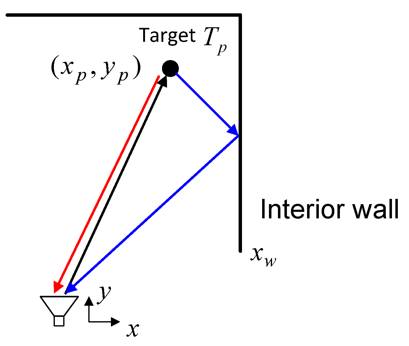
While the original signals reflect once or more times at the walls, the target returns at different propagation paths will be received with different delays. As shown in Figure 1, in the scenario of radar detection, we consider the dominant multipath component generated by the reflections at the internal surface. As indicated by the black and blue arrows, the signal is directly transmitted from the transceiver to the target, denoted by $T_p$, and then the scattered echo reflects back to the transceiver and vice versa. The direct return path is indicated by the red arrow. Assuming the geometry information is accessible, the time delays corresponding to the different multipath returns can be accurately acquired according to geometric relationships.

When there exists one direct path and $K-1$ indirect paths, the signal propagation model can be considered as the superposition of all propagation paths and formulated as [20]

$$\begin{array}{c}\hfill \tilde{\mathbf{y}}={\mathbf{\Phi }}_1{\mathbf{w}}_1+{\mathbf{\Phi }}_2{\mathbf{w}}_2+\cdots +{\mathbf{\Phi }}_K{\mathbf{w}}_K,\end{array}$$

(4)

where ${\mathbf{\Phi }}_k\in {\mathcal{C}}^{MN\times N_x{N}_y}$ and ${\mathbf{w}}_k\in {\mathcal{C}}^{N_x{N}_y}$ with $k\in \{1,\cdots K\}$ represent the sensing matrix and the complex reflectivities mentioned in Section 2.1 of the kth propagation path, respectively. When $k=1$, ${\mathbf{\Phi }}_k$ and ${\mathbf{w}}_k$ correspond to the direct path. In addition, the remaining ${\mathbf{\Phi }}_k$ and ${\mathbf{w}}_k$ correspond to the indirect path, where the elements of ${\mathbf{\Phi }}_k$ are phase terms, similar to (3), containing the corresponding time delay. It is worth mentioning that the elements of target reflectivity vectors ${\mathbf{w}}_k,k\in \{1,\cdots K\}$ have the same nonzero support on all propagation paths regardless of the different reflectivity coefficients.

Since the measurements of different propagation paths generally cannot be solved in TWRI, to overcome this difficulty, we rewrite (4) as

$$\begin{array}{cc}\hfill \tilde{\mathbf{y}}& =\mathbf{\Psi }\tilde{\mathbf{w}}+\mathsf{ϵ},\hfill \end{array}$$

(5)

$$\begin{array}{cc}\hfill \tilde{\mathbf{w}}& ={[{\mathbf{w}}_1,\cdots ,{\mathbf{w}}_K]}^T\in {\mathcal{C}}^{N_x{N}_{y}K},\hfill \end{array}$$

(6)

$$\begin{array}{cc}\hfill {\mathbf{w}}_k& =[w_{k1},\cdots ,w_{k,NxNy}]\in {\mathcal{C}}^{1\times N_x{N}_y},\hfill \end{array}$$

(7)

where $\tilde{\mathbf{y}}\in {\mathcal{C}}^{MN}$ denotes the measurement data vector, $\mathbf{\Psi }=[{\mathbf{\Phi }}_1,\cdots ,{\mathbf{\Phi }}_K]\in {\mathcal{C}}^{MN\times N_x{N}_{y}K}$ denotes the joint sensing matrix, and $\tilde{\mathbf{w}}$ denotes the combined complex reflectivity vector. For generalization, (2) plus a measurement noise vector $\mathsf{ϵ}\in {\mathcal{C}}^{MN}$ is considered as the measurements.

Within the CS framework, only a portion of the full measurements is used for high-quality sparse reconstruction. Therefore, we first decrease the amount of data collected. Mathematically, the data reduction operation is equivalent to implementing a measurement or downsampling matrix $\mathbf{D}\in {\mathcal{R}}^{J\times MN}$ on the total measurements, where $J\ll MN$ is the number of reduced measurements. A binary measurement matrix $\mathbf{D}\in {\{0,1\}}^{J\times MN}$ is a proper option for the stepped-frequency radar system in this article [20]. Therefore, the measurement vector after undersampling $\overline{\mathbf{y}}\in {\mathcal{C}}^J$ can be given by

$$\begin{array}{c}\hfill \overline{\mathbf{y}}=\mathbf{D}\tilde{\mathbf{y}}=\mathbf{D}\mathbf{\Psi }\tilde{\mathbf{w}}+\mathbf{D}\mathsf{ϵ}=\mathbf{A}\tilde{\mathbf{w}}+\widetilde{\mathsf{ϵ}},\end{array}$$

(8)

$$\begin{array}{c}\hfill \mathbf{A}=\mathbf{D}\mathbf{\Psi }\in {\mathcal{C}}^{J\times N_x{N}_y},\end{array}$$

(9)

$$\begin{array}{c}\hfill \widetilde{\mathsf{ϵ}}=\mathbf{D}\mathsf{ϵ}\in {\mathcal{C}}^J,\end{array}$$

(10)

where $\mathbf{A}$ is the dictionary matrix.

3. Clustered Bayesian Compressive Sensing

Direct application of the multi-task clustered BCS algorithm [17] for scene reconstruction in TWRI is not feasible due to the non-resolvability of the measurements corresponding to different propagation paths. To address the limitation of unresolvable measurements, a novel clustered BCS is devised as follows.

3.1. Sparse Prior

To improve the group sparsity across the multiple propagation paths, a Bernoulli–Gaussian distribution, also named a spike-and-slab prior [22,23], is incorporated in the elements of the reflectivity vector $\tilde{\mathbf{w}}$,

$$\begin{array}{c}\hfill p\left({\overline{\mathbf{w}}}_l\right|\mathsf{\pi },\mathsf{\beta })=\prod _{k=1}^K\left[(1-{\pi }_l)\delta \left(w_{kl}\right)+{\pi }_l\mathcal{CN}\left(w_{kl}\right|0,{\beta }_l^{-1})\right],\end{array}$$

(11)

where ${\overline{\mathbf{w}}}_l={[w_{1l},\cdots ,w_{Kl}]}^T$ with $l\in [1,\cdots ,N_x{N}_y]$, ${\pi }_l$ is the prior probability of the lth pixel taking nonzero value. The entry is therefore more likely to be zero if the mixing weight ${\pi }_l$ is small, whereas a larger ${\pi }_l$ usually results in a nonzero entry. Additionally, ${\beta }_l$ is the precision (inverse variance) of complex Gaussian distribution, and $\delta (·)$ is the Dirac delta function.

To acquire an analytical inference, the product of two latent variables ${\overline{\mathbf{w}}}_l=z_l{\mathsf{\theta }}_l$ is used to follow the pdf in (11) and express their joint pdf as [17],

$$\begin{array}{cc}\hfill p({\mathsf{\theta }}_l,z_l)& =\prod _{k=1}^K{\left[\mathcal{CN}\left({\theta }_{kl}\right|0,{\beta }_l^{-1})\right]}^{z_l}{\pi }_l^{z_l}{(1-{\pi }_l)}^{1-z_l},\hfill \end{array}$$

(12)

where ${\mathsf{\theta }}_l={[{\theta }_{1l},\dots ,{\theta }_{Kl}]}^T$, $z_l$ is a binary variable, and $z_l=0$ indicates that the lth pixel has a value of zero. It is evident that the group sparsity across the K paths is characterized by the same $z_l$ for the lth pixel. Consequently, all scattering coefficients in the lth pixel share the same ‘on’ or ‘off’ pattern. Furthermore, the values of all coefficients ${\mathsf{\theta }}_l$ in the lth pixel are generally different, due to diverse propagation paths [20].

A Gamma prior, conjugate to the Gaussian distribution, is incorporated in posterior ${\beta }_l$ to make it trackable. Thus, ${\beta }_l$ can be expressed as

$$\begin{array}{c}\hfill {\beta }_l\sim \mathrm{Gamma}(a,b),\end{array}$$

(13)

where $l\in [1,\cdots ,N_x{N}_y]$, and a and b are hyperparameters. In particular, this nonparametric hierarchical structure makes the model infer the precision ${\beta }_l$ automatically. For generalization, the additive noise is supposed to exhibit a Gaussian distribution, i.e., $\widetilde{\mathsf{ϵ}}\sim \mathcal{CN}(0,{\alpha }^{-1}{\mathbf{I}}_J).$ Similarly, a Gamma prior is incorporated in $\alpha$ to make the posterior distribution analytical, i.e., $\alpha \sim \mathrm{Gamma}(c,d)$, where c and d are hyperparameters.

3.2. Clustered Prior

To take advantage of the dependency structure between pixels, we consider three kinds of sparsity patterns, namely Pattern 0 (“strong rejection”), Pattern 1 (“weak rejection”), and Pattern 2 (“strong acceptance”). In the underlying TWRI problem, a 2-D imaging scene is considered, as shown in Figure 2. An auxiliary variable ${\kappa }_i=\sum {\mathbf{z}}_{{\eta }_l}$ is defined according to the total number of nonzero pixels adjacent to the ith pixel under test and introduces a new nonlinear function $\mathcal{F}$ in terms of ${\kappa }_l$. To reduce inference time, we incorporate a Beta prior into weights ${\pi }_l$ according to the clustered patterns. The Beta prior exhibits conjugately to the Bernoulli distribution and has three types of parameters ${\{e_i,f_i\}}_{i=0}^2$.

Strong rejection [Pattern 0]: For a small $\mathcal{F}\left({\kappa }_l\right)$, it implies that most or all of the neighboring pixels are zero. Therefore, there is a high likelihood that the lth test pixel will be equal to zero. In this instance, $e_0<f_0$ is used in prior Beta$\left({\pi }_l\right|e_0,f_0)$ to recommend a low value of ${\pi }_l$ for rejecting this pixel.

Weak rejection [Pattern 1]: For a comparative $\mathcal{F}\left({\kappa }_l\right)$, it implies the amounts of adjacent pixels with zero and nonzero values are comparable. In this instance, the likelihood that the lth test pixel is equal to zero or nonzero value is the same. Thus, $e_1=f_1$ is used in the prior $\mathrm{Beta}\left({\pi }_l\right|e_1,f_1)$ to impose prior without information on ${\pi }_l$.

Strong acceptance [Pattern 2]: For a large $\mathcal{F}\left({\kappa }_l\right)$, it suggests that most or all of the neighboring pixels are non-zero. To enforce the target scene continuity, the lth pixel is required to be a non-zero value. In this instance, $e_2>f_2$ in the prior $\mathrm{Beta}\left({\pi }_l\right|e_2,f_2)$ recommends a high value of ${\pi }_l$ to adopt this pixel.

3.3. Posterior Inference

We use a Markov Chain Monte Carlo (MCMC) sampler to conduct the Bayesian inference of the algorithm. For simplicity, the set of the hyperparameters is defined as $\Xi \stackrel{\Delta }{=}\{a,b,c,d,\mathbf{e},\mathbf{f}\}$, where $\mathbf{e}\stackrel{\Delta }{=}\{e_0,e_1,e_2\}$ and $\mathbf{f}\stackrel{\Delta }{=}\{f_0,f_1,f_2\}$. The set of random variables is defined as $\mathbf{\Theta }\stackrel{\Delta }{=}\{\mathsf{\theta },\mathbf{z},\mathsf{\pi },\alpha ,\mathsf{\beta }\}$. Thus, the specific form of the joint pdf can be given by

$$\begin{array}{cc}\hfill p\left(\overline{\mathbf{y}},\mathbf{A},\mathbf{\Theta }|\Xi \right)& =\mathcal{CN}\left(\overline{\mathbf{y}}\right|\mathbf{A}(\mathsf{\theta }\circ \mathbf{z}),{\alpha }^{-1}{\mathbf{I}}_J)\mathrm{Gamma}\left(\alpha \right|c,d)\hfill \\ \hfill & \times \prod _{l=1}^{N_x{N}_y}\prod _{k=1}^K{\left[\mathcal{CN}\left({\theta }_{kl}\right|0,{\beta }_l^{-1})\right]}^{z_l}{\pi }_l^{z_l}{(1-{\pi }_l)}^{1-z_l}\hfill \\ \hfill & \times \prod _{l=1}^{N_x{N}_y}\mathrm{Beta}\left({\pi }_l\right|\mathbf{e},\mathbf{f})\mathrm{Gamma}\left({\beta }_l\right|a,b).\hfill \end{array}$$

(14)

According to the conjugate relationship, an analytical method will be used to determine the posterior distribution of each random variable. Since the difference between the proposed algorithm and the clustered MT-BCS lies only in the measurements, the updated variables independent of the measurements will share the same updated equations. Here we further present the inferences of those variables which are dependent on the measurements and have different updated formulations in [17].

From the signal model, it is observed that only the variables $\{\mathsf{\theta },\mathbf{z},\alpha \}$ are related to the observation data $\overline{\mathbf{y}}$. We first update the paired variables $(\mathsf{\theta },\mathbf{z})$. The conditional pdf is sampled iteratively by the paired Gibbs sampler and given by

$$\begin{array}{c}\hfill p(z_l,{\mathsf{\theta }}_l|{\theta }_{\setminus l},{\mathbf{z}}_{\setminus l},\overline{\mathbf{y}})=p\left({\mathsf{\theta }}_l\right|z_l,{\mathsf{\theta }}_{\setminus l},{\mathbf{z}}_{\setminus l},\overline{\mathbf{y}})p\left(z_l\right|{\mathsf{\theta }}_{\setminus l},{\mathbf{z}}_{\setminus l},\mathbf{y}),\end{array}$$

(15)

where ${\mathsf{\theta }}_{\setminus l}$ and ${\mathbf{z}}_{\setminus l}$ represent $\mathsf{\theta }$ minus the variable vector ${\mathsf{\theta }}_l$ and $\mathbf{z}$ minus the variable $z_l$, respectively. The logistic function is employed to calculate the analytical likelihood $p(z_l=1|{\mathsf{\theta }}_{\setminus l},{\mathbf{z}}_{\setminus l},\overline{\mathbf{y}})$ [17] which can be expressed as

$$\begin{array}{cc}\hfill & p(z_l=1|{\mathsf{\theta }}_{\setminus l},{\mathbf{z}}_{\setminus l},\overline{\mathbf{y}})=\frac{1}{1+e^{-u}},\hfill \end{array}$$

(16)

where u is given by

$$\begin{array}{cc}\hfill u& =\frac{K}{2}log{\beta }_l+\frac{1}{2}log\left|{\Sigma }_l\right|+\frac{1}{2}{\overline{\mathbf{y}}}_{\setminus l}^H{\overline{\mathbf{A}}}_l{\Sigma }_l^{-1}{\overline{\mathbf{A}}}_l^H{\overline{\mathbf{y}}}_{\setminus l}\hfill \\ \hfill & +log{\pi }_l-log(1-{\pi }_l)\hfill \end{array}$$

(17)

$$\begin{array}{cc}\hfill {\Sigma }_l& ={(\alpha {\overline{\mathbf{A}}}_l^H{\overline{\mathbf{A}}}_l+{\beta }_l)}^{-1},\hfill \end{array}$$

(18)

and ${\overline{\mathbf{A}}}_l=[{\mathbf{A}}_{l1},\cdots ,{\mathbf{A}}_{lK}]\in {\mathcal{C}}^{J\times K}$ denotes the collection of the lth column in each dictionary matrix ${\left\{{\mathbf{A}}_k\right\}}_{k=1}^K$.

The conditional distribution of $p\left({\mathsf{\theta }}_l\right|z_l=1,{\mathsf{\theta }}_{\setminus l},{\mathbf{z}}_{\setminus l},\overline{\mathbf{y}})$ can be denoted by

$$\begin{array}{cc}\hfill p\left({\mathsf{\theta }}_l\right|z_l=1,{\mathsf{\theta }}_{\setminus l},{\mathbf{z}}_{\setminus l},\overline{\mathbf{y}})& =\mathcal{CN}\left({\mathsf{\theta }}_l\right|\alpha {\Sigma }_l{\mathbf{A}}_l^H{\overline{\mathbf{y}}}_{\setminus l},{\Sigma }_l).\hfill \end{array}$$

(19)

As depicted in Section 3.2, each element ${\pi }_l$ is selected based on the sparsity pattern, namely ${\pi }_l$ is allocated as ${\pi }_l^{\left(q\right)}$ according to different pattern $q\in \{0,1,2\}$. For a specific sparsity pattern q, a posterior distribution is obtained analytically owing to the Beta distribution on ${\pi }_l$ and given by

$$\begin{array}{c}\hfill p\left({\pi }_l^{\left(q\right)}\right|\mathbf{e},\mathbf{f},\mathbf{z})=\mathrm{Beta}(e_q+{\kappa }_l+z_l,f_q+{\nu }_l+1-{\kappa }_l-z_l),\end{array}$$

(20)

where $l\in \{1,\cdots ,N_x{N}_y\}$, and ${\nu }_l$ is the length of ${\mathbf{z}}_{{\eta }_l}$. In the two-dimensional signal instance shown in Figure 2, ${\nu }_l=8$ indicates that each pixel is taken into account along with its 8 closest neighbors.

With the help of the conjugate relationship between the Gaussian and Gamma distributions, the analytical posterior distribution of the precision variable ${\beta }_l$ is obtained as

$$\begin{array}{c}\hfill p\left({\beta }_l\right|a,b,\mathsf{\theta })=\mathrm{Gamma}\left({\beta }_l\right|\tilde{a},\tilde{b}),\end{array}$$

(21)

where $\tilde{a}=a+(K/2)$, $\tilde{b}=b+{\sum }_l({\theta }_{lk}^2/2)$, and $l\in [1,\cdots ,N_x{N}_y]$.

For the noise precision $\alpha$, we acquire the posterior distribution as

$$\begin{array}{c}\hfill p\left(\alpha \right|c,d,\mathbf{y},\mathbf{A},\mathsf{\theta },\mathbf{z})=\mathrm{Gamma}\left(c+\frac{J}{2},d+\frac{\parallel \overline{\mathbf{y}}{-\mathbf{A}(\mathsf{\theta }\circ \mathbf{z})\parallel }^2}{2}\right).\end{array}$$

(22)

Algorithm 1 provides the entire procedure of the proposed clustered BCS algorithm. We employ the Gibbs sampler with consecutive sampling to infer the model parameters. It is observed that the computational complexity is $\mathcal{O}(J\times N_x{N}_y\times K^3\times N_{\mathrm{maxiter}})$, where $N_{\mathrm{maxiter}}$ is the maximum number of iterations. When the maximum number of iterations is reached, the algorithm stops and outputs the result.

Algorithm 1 Clustered BCS algorithm

Input:

Initialize $\Xi$ and $\mathbf{\Theta }$;

Assign $N_{\mathrm{maxiter}}$;

for $n=1,\cdots ,N_{\mathrm{maxiter}}$, do

for $l=1,\cdots ,N_x{N}_y$, do

update $z_l\sim p(z_l=1|{\mathsf{\theta }}_{\setminus l},{\mathbf{z}}_{\setminus l},\overline{\mathbf{y}})$ [Equation (16)];

update ${\mathsf{\theta }}_l\sim p\left({\mathsf{\theta }}_l\right|z_l=1,{\mathsf{\theta }}_{\setminus l},{\mathbf{z}}_{\setminus l},\overline{\mathbf{y}})$ [Equation (19)];

update ${\pi }_l\sim p\left({\pi }_l^{\left(q\right)}\right|\mathbf{e},\mathbf{f},\mathbf{z})$ [Equation (20)];

update ${\beta }_l\sim p\left({\beta }_l\right|a,b,\mathsf{\theta })$ [Equation (21)];

end for

update $\alpha \sim p\left(\alpha \right|c,d,\mathbf{y},\mathbf{A},\mathsf{\theta },\mathbf{z})$ [Equation (22)];

end for

Output:

$\mathsf{\theta }$ and $\mathbf{z}$.

4. Results

This section presents simulations and experimental results to verify the correctness of the proposed radar imaging algorithm. The following values of the parameters are assumed in the experiments: hyperparameters a, b, c and d are equal to ${10}^{-6}$, $(e_0,f_0)=(1/J,1-1/J)$ for strong rejection, $(e_1,f_1)=(1/J,1/J)$ for weak rejection, and $(e_1,f_1)=(1-1/J,1/J)$ for strong acceptance. The function $\mathcal{F}\left({\kappa }_l\right)$ is a step function, which takes a zero value with ${\kappa }_i=0$ for strong rejection, an infinite value for strong acceptance with ${\kappa }_l\ge 4$, or a comparative value for weak rejection. 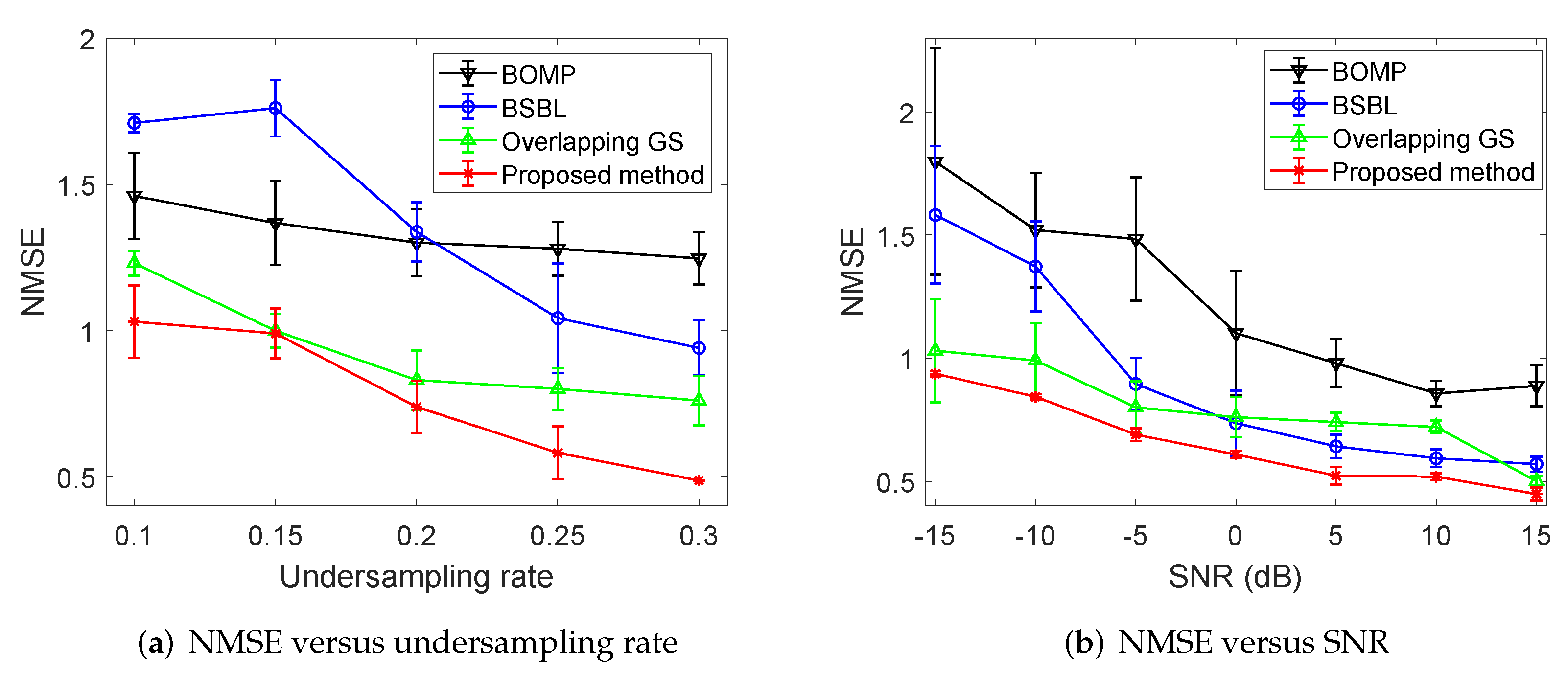The $N_{\mathrm{maxiter}}$ is set as 200, and the sample with the maximum marginal likelihood among the last 20 samples are selected as the estimation of $\mathbf{w}$ [17]. To evaluate the reconstruction results, the normalized mean square error (NMSE) $\parallel \widehat{\mathbf{w}}-{\mathbf{w}}_{\mathrm{gen}}{\parallel }_2^2/{\parallel {\mathbf{w}}_{\mathrm{gen}}\parallel }_2^2$, where $\widehat{\mathbf{w}}$ is the estimate of the ${\mathbf{w}}_{\mathrm{gen}}$, is introduced as the performance index. The results of the conventional (BP) algorithm [24], overlapping GS method [15], BOMP [20] and BSBL [25] are also presented for comparison. All the results are implemented on the PC with CPU (Intel Core i7-10700K) using Matlab R2020a.

4.1. Simulated Dataset

Simulations were performed for a monostatic radar with a 77-element monostatic ULA. The spacing between elements is set as $1.9$ cm. Each element transmits a stepped-frequency signal and receives the target returns. The transmitted wave consists of 200 equally spaced frequency steps and covers the 1 GHz to 3 GHz. The detailed parameters are given in

Table 2. Simulation parameters.

Parameters	Value
Initial frequency	1 GHz
Cut-off frequency	3 GHz
Bandwidth	2 GHz
Number of steps	500
Step frequency	10 MHz
Number of elements	77
Element interval	$1.9$ cm

. The middle of the antenna array is regarded as the original point. The front wall is $2.44$ meters away from the antenna array, but it is not considered in the scenario for simplicity. The locations of the two side walls are around $\pm 1.83$ m crossrange, whereas the location of the back wall, parallel to the antenna array, is $6.37$ m downrange. The scattering coefficient of the direct path is determined according to $\mathcal{N}(0,1)$. In addition, the signal amplitudes of the received returns decrease as the distance increases. A target occupying $Q=8$ contiguous pixels is considered, as shown in Figure 3a. The received signal includes a total of $K=4$ paths, consisting of the direct echo as well as indirect paths reflected on the surfaces of the three walls. To simulate the real scenario, the measurements with an SNR of 0 dB plus additive Gaussian noise are employed for simulations. When using the classical BP method, all available data are used; however, only a quarter of all frequencies are chosen at random for the CS-based imaging.

We first present the reconstructed image using the BP algorithm in Figure 3b in which three ghosts exist due to the three indirect paths from three interior walls, respectively. It is evident that the BP-based algorithm is unable to properly rebuild the scenario and distinguish the true target from the ghosts. The reconstruction result contains a much higher amount of clutter. In addition, the resolution of the BP algorithm is $0.75$ m owing to the 2 GHz band. Constrained by the Rayleigh boundary, the exact shape of the target is hard to obtain. In these CS-based approaches, it is observed that these ghosts from multipath propagations can be effectively alleviated due to the exploitation of group sparsity structure, as depicted in Figure 3b–f. The reconstruction result using the BOMP method is provided in Figure 3c, and it is clear that several fake pixels are located around the real positions, even though the true sparsity number is used in advance. Figure 3d depicts the imaging result based on the BSBL method. It can be found that the reconstruction result is similar to the ground truth, whereas some spurious isolated pixels occur because of the target structure being neglected. Figure 3e gives the reconstructed result using the overlapping group CS algorithm. It is clear that the overlapping group CS algorithm can reconstruct and capture the target shape, whereas it leads to some fake pixels around the real locations owing to the inappropriate overlapping partition. Figure 3f suggests that the proposed method can successfully reconstruct the target with a continuously clustered structure and effectively suppress the separated and false targets by enforcing the clustered prior. The improvements of the proposed method are also verified by the NMSE values, which are, respectively, $1.13$ in the BOMP method, $0.78$ in the BSBL method, $0.82$ in the overlapping GS method, and $0.58$ in the proposed algorithm. In addition, we also provide the executive time comparisons among these methods, as shown in

Table 3. Executive time comparisons.

	BOMP	BSBL	Overlapping GS	Proposed Algorithm
Runtime (s)	0.45	175.5	65.5	180.3

. It is observed that the BOMP method has the smallest runtime, and the runtime is less than 1 s, because the used iteration number of this method is exactly the sparsity number. The executive time in the proposed method is comparable to that in the BSBL method.

Reconstruction Performance Analysis

The reconstruction performance is described by calculating the NMSE between the true and estimated position of the target. To further prove the correctness of the clustered BCS method, we show the NMSE versus the undersampling rate and the NMSE versus SNR, respectively, in Figure 4a,b. In this simulation, all other parameters are kept in the above simulation in Section 4.1. The ratio varies from $10\%$ to $30\%$ with the step of $5\%$. The result comparison of NMSE versus undersampling is shown in Figure 4a. It is clear that the NMSEs generally decreases with increased undersampling rates. The NMSEs in the proposed method are generally lower than those in other methods across the undersamping ratio. It is observed that the reconstructed NMSE would reduce to $0.48$, when the undersampling rate approach $0.3$, compared to an NMSE of 0.76 in the Overlapping GS method, 0.94 in the BSBL method, and 1.24 in the BOMP method even with a known sparsity number. The reason for the superior performance of the proposed method over these methods may benefit from the fact that the proposed method combines group sparsity with clustered structure into the model for high-resolution imaging.

We also investigate the effect of additive noise on the performance of the clustered BCS method. All other parameters are kept in the above simulation in Section 4.1. The SNR ranges from $-15$ dB to 15 dB with the step of 5 dB. It is demonstrated in Figure 4b that the reconstructed NMSEs of all algorithms generally increase with the increases of the noise power. It is observed that the BOMP method seems more sensitive to the noise power, and generally has the highest NMSEs as compared to the other three methods, even with a known sparsity number. The main reason could be that there is the high coherence in the measurement matrix. However, the proposed method offers more robustness to noise power and shows smaller NMSEs across SNRs, and the NMSE in the proposed method is reduced to $0.44$, compared to $0.50$ in the overlapping GS method, $0.56$ in the BSBL method and $0.88$ in the BOMP method, when the SNR approaches 15 dB.

4.2. Experimental Dataset

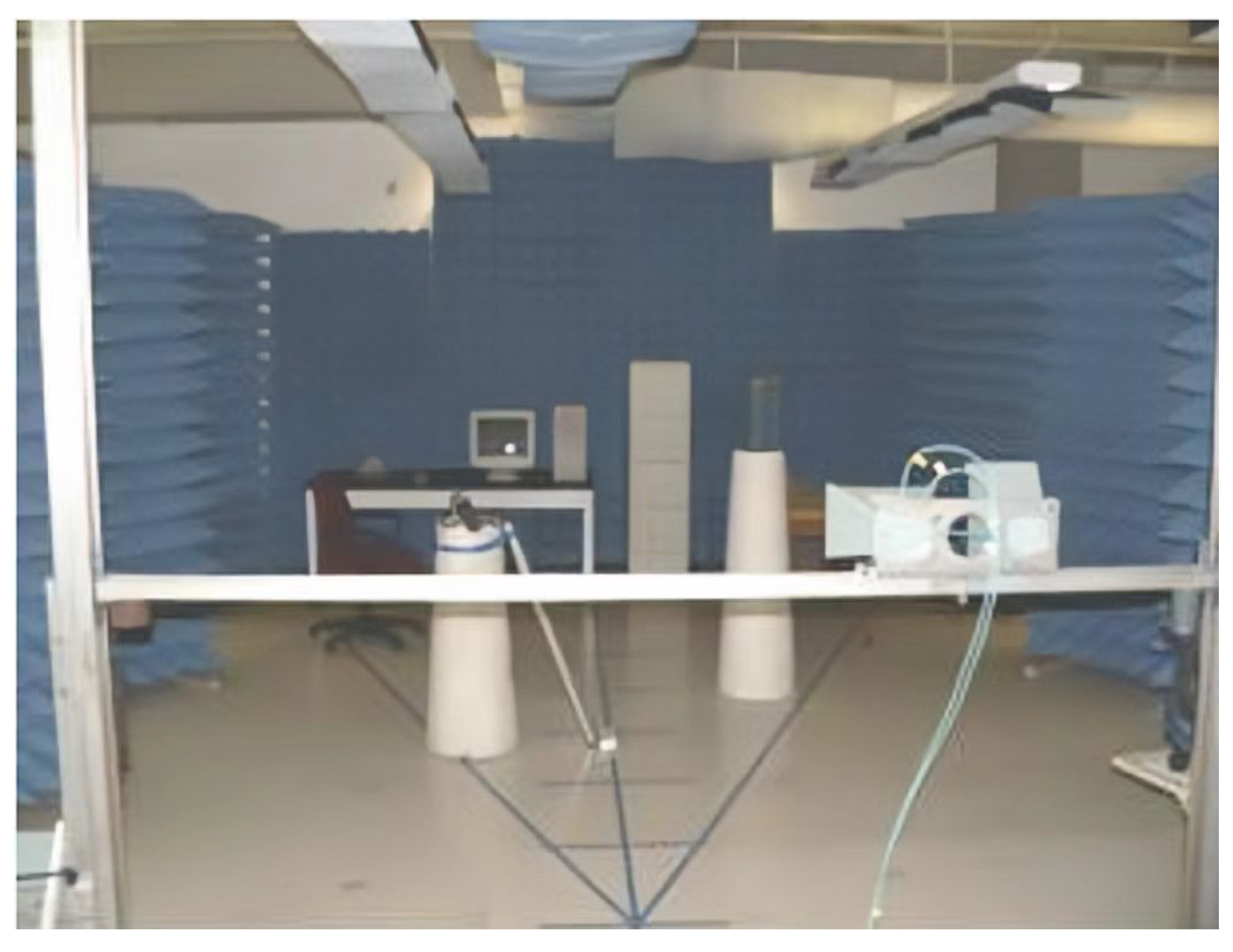
To verify the proposed radar imaging algorithm experimentally, the experimental data were collected at the Radar Imaging Lab, Villanova University. The parameters of the antenna array and the positions of the concrete walls are the same in the simulation. In particular, the difference is that the stepped-frequency signal contains 801 frequency steps evenly distributed from 1 GHz to 3 GHz. An aluminum pipe (length of 61 cm and diameter of 7.6 cm) was set upright on a foam pedestal (height of 1.2 m) at a 3.67 m downrange and 0.31 m crossrange. The protruding corner causing multipath is located at the upper right area at 3.4 m crossrange and 4.57 m downrange. We put RF absorbing material on the surfaces of the side walls to eliminate multipath from these two walls; however, the surfaces of the back wall and protruding corner are uncovered. The wall clutter is well removed so that only target echoes are considered in the experiments [20]. The overall experimental scene is shown in Figure 5.

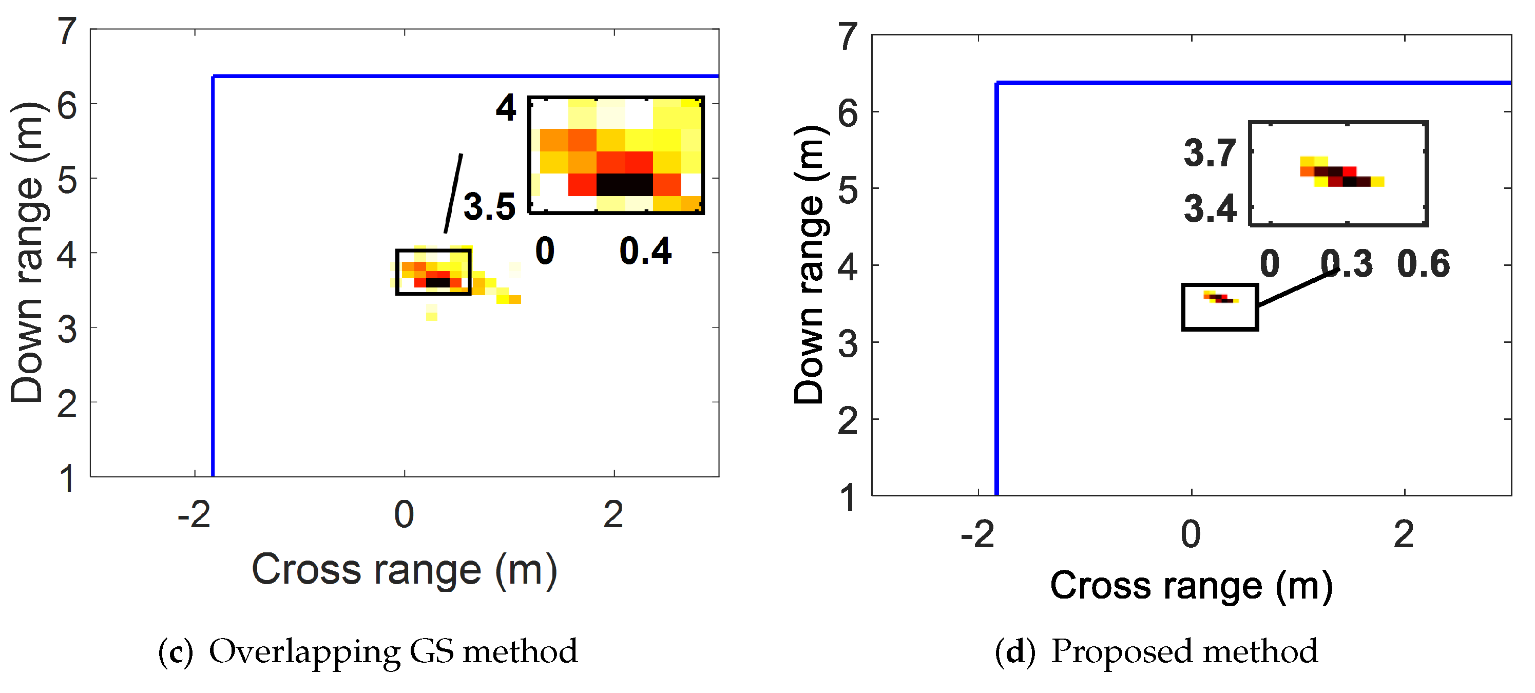
We first present the conventional beamformed result using all available data in Figure 6a. It can be observed that the ghosts caused by the uncovered surfaces are clear and distinct. Therefore, we simply analyze the cases where the reflection points are on the uncovered surfaces in the following. To reduce the time of data collection, one fourth of the array elements and the frequencies are employed in the CS reconstruction. Since the sparsity number in this dataset is hard to know, we do not consider using the BOMP mentioned in the simulation above for comparison. As depicted in Figure 6b, There exist a lot of separated pixels in the reconstruction result of the BSBL algorithm. From Figure 6c,d, it is evident that the overlapping GS and the proposed algorithm yield fewer cluttered images and better target depictions. However, it appears that there are numerous fake pixels around the real pixels due to the overlapping partition. Similar to [20], the metric of relative clutter peak (RCP), which is defined as the maximum target amplitude divided by the maximum clutter amplitude, is introduced to evaluate the imaging quality. The clutter region is defined as the space inside the indoor scenes, excluding a circle with a radius of 10 cm at the known target position. The RCP, respectively, evaluates $44.3$ dB, $40.39$ dB, and 48.62 dB for the BSBL, the overlapping GS methods as well as the proposed algorithms.

5. Conclusions

This paper focused on the problem of multipath exploitation for TWRI in view of sparsity-based reconstruction methods. The underlying idea is to take advantage of both the group sparsity due to the multipath propagations and the continuous clustered structure on the targets. A novel CS-based multipath exploitation clustered BCS approach for image reconstruction was proposed. Benefiting from the data-driven capability of the nonparametric hierarchical Bayesian model, the proposed method achieved high-resolution TWRI without any prior information about the targets, such as shapes, sizes, and numbers. In addition, it is worth mentioning that the proposed algorithm is not restricted to the ULA application, and can be generalized to any other array shapes.

The proposed method has the capability of acquiring high-resolution target images with free ghosts in the indoor multipath propagation environment, and thus it provides opportunities to better capture indoor messages through the wall, such as the shape of indoor stationary items, locations of indoor human targets, etc. It would also prompt further feature extraction and recognition of indoor targets behind the wall. Although the proposed method enables obtaining ghost-free high-resolution indoor targets image, the following challenges remain to be addressed in future work: (1) Prior knowledge of the number of propagation paths and their topology was assumed and provided for multipath exploitation; however, it is difficult to accurately acquire this information in practice. Therefore, it would be a challenging issue to acquire ghost-free high-resolution TWRI for multipath exploitation, when the indoor topology is inaccurate or completely unknown. (2) A centralized scheme with a uniform linear array was used where all measurements are available at a single processing node. However, a decentralized approach would be beneficial for practical purposes. Each of the nodes carries out part of the reconstruction while communicating with the other units. This results in the simpler and more flexible operation of the TWRI system and avoids a single point of failure. Proper algorithm design should ensure that the reconstruction quality is on par with centralized processing.

In summary, it is still quite challenging for the high-resolution TWRI in the multipath-propagation environment for practical purposes due to the diversities and complexities of the indoor configurations.