Article

The Dual Effects of Environmental Regulation and Financial Support for Agriculture on Agricultural Green Development: Spatial Spillover Effects and Spatio-Temporal Heterogeneity

1
School of Management, Jiangsu University, Zhenjiang 212013, China
2
Research Centers of Green Development and Environmental Governance, Jiangsu University, Zhenjiang 212013, China
*
Author to whom correspondence should be addressed.
Appl. Sci. 2022, 12(22), 11609; https://doi.org/10.3390/app122211609
Submission received: 21 October 2022 / Revised: 9 November 2022 / Accepted: 11 November 2022 / Published: 15 November 2022
(This article belongs to the Section Green Sustainable Science and Technology)

Abstract

:
Environmental regulation and financial support for agriculture are regarded as important means to promote agricultural green development. Based on provincial panel data of 31 provinces in China between the years 2000 and 2020, this paper explores the interactive effect, spatial spillover effect and spatio-temporal heterogeneity of environmental regulation and financial support for agriculture on agricultural green development. The empirical conclusions are as follows: (1) The level of agricultural green development increases year by year with a spatial characteristic of high in the east and low in the west. Moreover, there is a spatial spillover effect of agricultural green development with spatiotemporal heterogeneity. (2) Environmental regulation would not only reduce the level of local agricultural green development but also inhibit the adjacent regions, which is contrary to the impact of financial support for agriculture. (3) The interactive relationship of environmental regulation and financial support for agriculture has a spatial spillover effect on agricultural green development, which is more significant in the systematization stage of agricultural green development and most significant in the east-middle region.

1. Introduction

Agricultural green development is one critical path of China’s ecological civilization construction and also the inevitable approach to achieving the target of agricultural carbon peaking and carbon neutrality strategy [1]. However, the current agricultural extensive management mode in China, which mainly relies on resource consumption with high emissions, has not been changed and caused serious problems of agricultural non-point source pollution and ecological degradation [2]. As such, China has issued policies to address agricultural green development. First, an overall layout of ecological, agricultural and other functional spaces is formulated. Second, the environmental pollution bottom line of agricultural green development and environmental protection responsibility target assessment has been strictly executed by the agricultural and rural comprehensive administrative law enforcement team to promote environmental regulation. Third, the funds to support agricultural green development have been increased in recent years. Thus, to realize the fundamental reform of extensive agricultural development mode and promote agricultural green development, both financial support for agriculture and environmental regulation are essential [3].
Current research also shows that financial support for agriculture and environmental regulation are the main measures to promote agricultural green development [4]. On the one hand, financial support for agriculture could promote not only the local level of agricultural green development but also that of other adjacent regions. This is because the local government would provide a series of subsidies and incentives to local agricultural operators for emission reduction and technological innovation [5,6]. It will promote the generation of new technologies for agricultural green development; accordingly, the level of agricultural green development in adjacent regions would also be promoted with knowledge diffusion and technology spillover [7,8]. In addition, due to the differences in resource endowments and policies of financial support for agriculture among different areas, the influence mechanism of financial support for agriculture on agricultural green development has shown different spatial effects in different areas [9]. Moreover, the performance appraisal objectives for local governments have varied from gold and silver mountains to clear water and green mountains with the target of carbon peaking and carbon neutrality strategy. As such, local governments have reduced carbon emissions through financial environmental expenditure, which has a demonstration function to their adjacent regions [10,11,12]. On the other hand, environmental regulation is also regarded as an important element for promoting agricultural green development [12]. Based on the “strong porter hypothesis”, reasonable environmental regulation could promote the upgrading of agricultural industrial structure and technical innovation in the local area, reducing agricultural pollution and agricultural carbon emissions. Moreover, due to the spillover characteristics of agricultural pollution, local environmental regulation also restrains the transfer of agricultural pollution to adjacent regions and indirectly improves their agricultural environment [13]. However, as the cost-following theory suggested that strict environmental regulation would be higher than the input cost of agricultural development, which could not improve the inefficiency of agriculture, but aggravate both local and adjacent agricultural pollution [9,14], thus finally inhibiting agricultural green development in both local and adjacent regions.
Therefore, this paper explores the relationship between environmental regulation, financial support for agriculture and agricultural green development from a spatial spillover perspective. What are the temporal and spatial evolution characteristics of agricultural green development? Are there any interactive effects between environmental regulation and financial support for agriculture on agricultural green development? Is there any spatial-temporal heterogeneity in the influence of environmental regulation and financial support for agriculture on agricultural green development?
The paper is arranged as follows. Section 2 is materials and methods, which describe the research hypotheses, model set, data and measurement of core variables. Section 3 are the results, focusing on the analysis of the spatial-temporal evolution characteristics of agricultural green development, spatial Dubin model regression results and spatial effect decomposition. This section also conducts further research on spatial-temporal heterogeneity in the impact of environmental regulation and financial support for agriculture on agricultural green development. Additionally, the robustness test is carried out by replacing the spatial weight matrix, transforming the estimation method and adding control variables. Section 4 draws conclusions and implications.

2. Materials and Methods

2.1. Research Hypotheses

2.1.1. The Spatial Spillover Effect of Environmental Regulation on Agricultural Green Development

Agricultural green development mostly depends on the formulation and enforcement of environmental regulations. Research on the spatial spillover effects of environmental regulation on agricultural green development mainly focused on three perspectives. First, according to the “strong porter hypothesis”, the stronger the intensity of environmental regulation, the more conducive to curbing agricultural carbon emissions [15]. Moreover, the variation of local government’s environmental governance level from bottom competition to definite competition is conductive to produce a significance spatial spillover effect on the environmental governance of adjacent regions [16]. For example, to deal with ecological degradation, the G7 countries have adopted environmental regulations and various measures to reduce carbon emissions [11]. Moreover, the public voluntary environmental regulation also has a positive effect in promoting agriculture green development in adjacent regions through the element flow of labor, technology and other production factors in the local area [7]. Second, as the agricultural carbon emission trading market is still in the exploratory stage, market-motivated environmental regulation shows no significant impact on both local and adjacent regions [7]. Furthermore, local governments also excessively emphasize the importance of environmental regulation means while ignoring technology and other means, thus weakening the positive externalities of environmental governance, which hinder the communication and exchange of adjacent regions, resulting in the negative externalities of environmental governance. Previous research found that environmental regulation was characterized by an emphasis on treatment and light focus on prevention, which could not promote the development of agricultural technology and inhibit agricultural pollution emission [17]. That is, a negative spillover effect of environmental governance on the spatial environment would be generated [17,18]. Third, environmental regulation shows no significant impact on agricultural green production efficiency when measuring the investment amount of environmental governance [19] while showing a nonlinear “U-shaped” relationship by measuring agricultural pollution intensity [20]. Some countries have adopted high-intensity environmental regulation means [21]. Therefore, agricultural operators have to comply with relevant environmental regulation requirements and pay high environmental protection costs, which could be in conducive to promote agricultural green development in both local and adjacent regions. Thus, this paper puts forward the following hypothesis:
Hypothesis 1 (H1). 
Environmental regulation has a negative spatial spillover effect on agricultural green development; that is, local environmental regulation has a restraining effect on agricultural green development in adjacent regions.

2.1.2. The Spatial Spillover Effect of Financial Support for Agriculture on Agricultural Green Development

Relevant studies at home and abroad on the spatial spillover relationship between financial support for agriculture and agricultural green development have explored the two aspects. On the one hand, local financial support for agriculture could promote the agglomeration of information, technology and talents in the local region, which is conducive to the information exchange and knowledge spillover of the agricultural environment in the local region, as well as the diffusion of technology and knowledge in adjacent regions, promoting agricultural green development in both local and adjacent regions [6,7,8,9,10,11,12,13,14,15,16,17,18,19,20,21]. Additionally, with subsidies for delayed fertilization control, soil testing and formula fertilization, and R&D of energy-saving and environmental protection machinery technology, agricultural carbon emissions could be reduced, as well as the adjacent regions due to technology spillovers [22]. On the other hand, financial support for agriculture could promote competition in agricultural development industries between local and adjacent regions, which would increase agricultural carbon emission and inhibit agricultural green development by a high input of energy, fertilizers, pesticides, untreated agricultural wastewater containing nitrogen and phosphorus and other agricultural materials [5,6,7,8,9,10,11,12,13,14,15,16,17,18,19,20,21,22,23]. Furthermore, one region would gather more agricultural production resources which may have a siphoning effect on the adjacent regions, suppressing the adjacent regions’ level of agricultural green development [23]. Thus, this paper puts forward the following hypothesis:
Hypothesis 2 (H2). 
Financial support for agriculture has a spatial spillover effect on agricultural green development.

2.1.3. The Spatial Spillover Effect of Interaction between Environmental Regulation and Financial Support for Agriculture on Agricultural Green Development

Interaction between environmental regulation and financial support for agriculture on agricultural green development has been focused, which could be included the following two aspects. First, agricultural pollution governance investment and rural pollution control investment are proposed to be integrated into an index of agricultural ecological pollution control investment [24,25]. Second, suggestions for agricultural green development mainly include two aspects of environmental regulation and financial support for agriculture, such as rational intensity of fertilizer application, rewards for public participation in environmental regulation, agricultural green development funds and agricultural machinery input [5,6]. In addition, research also shows that the interaction between environmental regulation and financial support for agriculture has a spatial correlation with agricultural green development. First, local government would increase financial protection and economic expenditure on the regional agricultural environment. While adjacent regions could take advantage of geographical location to realize free riding on the environmental governance performance and then promote their agricultural green development. Second, excessive government funds to support agriculture would lead to local protectionism of environmental protection performance, which would hinder element flow with their adjacent regions, leading to negative externalities of environmental regulation, and then have a negative impact on the agricultural environment of adjacent regions. Flexible policy instruments are essential for ecological restoration [21]. Thus, this paper puts forward the following hypothesis:
Hypothesis 3 (H3). 
Interaction between environmental regulation and financial support for agriculture has a negative spatial effect on agricultural green development.
In conclusion, previous studies only pay attention to the single spatial spillover effect of environmental regulation and financial support for agriculture on agricultural green development, and only suggestion that environmental regulation and financial support for agriculture should be combined to promote agricultural green development has been proposed. As such, the spatial spillover effect of the interaction between environmental regulation and financial support for agriculture on agricultural green development should be explored from the empirical perspective. Based on these, this paper adopted China’s provincial panel data between the year of 2000 and 2020 to construct static and dynamic spatial Dubin models to test the spatial spillover effects, dual effects and spatio-temporal heterogeneity of environmental regulation and financial support for agriculture on agricultural green development.
Compared with the existing literature, the marginal contribution of this paper are as follows: (1) Further the current research from the perspective of the dual effect of environmental regulation and financial support for agriculture on the spatial spillover effect of agricultural green development, the static and dynamic spatial Dubin model was constructed to consider the interaction between environmental regulation and financial support for agriculture on the spatial spillover effect of agricultural green development. (2) Current research on regional heterogeneity is mainly divided into three areas: eastern, central and western, which would cut off the connection between adjacent provinces in the same region to some extent. As such, this paper refers to relevant research and divides the samples of the east-middle region, east-west region and middle-west region to more reasonably analyze the spatial heterogeneity.

2.2. Data and Methodology

2.2.1. Data

Considering data accessibility and integrity, this paper selects 31 provinces (including autonomous areas and municipalities while excluding Hong Kong, Macao, Taiwan, Diaoyu Island, the Sansha Islands and other areas given the lack of statistical data). in China as samples referring to the previous literature, which could fully reflect the whole and the regional agricultural green development in China., The data period is from the year of 2000 to 2020. The data mainly come from the China Rural Statistical Yearbook, China Statistical Yearbook, China Environmental Statistical Yearbook, China Construction Statistical Yearbook, Provincial Statistical Yearbook, China Statistical Yearbook of Science and Technology and statistical bulletin of cities. To ensure the reliability and continuity of the research results, invalid samples with missing data were eliminated. Additionally, based on the variation trend of the data, smoothing processing and interpolation method are adopted to fill in the missing data.

2.2.2. Spatial Weight Matrix Setting

As the spatial distance measurement among regions is the premise of spatial econometric analysis, this paper first conducts the geographical adjacency matrix (W) based on 31 provinces’ geographical locations and sets the geographical adjacency space weight matrix based on a binary algorithm, which is widely adopted. The matrix constructed is as follows:
  W i j = { 1 ,   i   w i t h   j   a d j a c e n t 0 , i   w i t h   j   n o n a d j a c e n t
In Equation (1), if there is a common boundary between province i and j, the value is 1; otherwise, the value is 0. Given Hainan province is an island, we set it with Guangdong province as mutually adjacent, referring to the previous research. The matrix row and standardization processing are carried out respectively, and i, j are denoted to measure the distance of region i and region j.

2.2.3. Spatial Autocorrelation Test

A spatial autocorrelation test is the basis for constructing a spatial Dubin model. The geographic space distribution characteristics with variables of environmental regulation, financial support for agriculture and agricultural green development are analyzed by autocorrelation test [25]. The absolute value of the global Moran’s I is denoted as the intensity of spatial correlation, in which the value range of Moran’s I is [−1, 0], indicating that there is a negative spatial correlation, while the value range of Moran’s I is [0, 1] indicating that there is a positive spatial correlation. The formula of I is as follows:
I = n i = 1 n j = 1 n w i j ( x i x ¯ ) ( x j x ¯ ) i = 1 n j = 1 n w i j i = 1 n ( x i x ¯ )  
In Equation (2), I is the global Moran’s I; n is the number of provinces; x i and x j   represents variables’ value of province i and j, respectively, and x ¯   is the average value of variables. w i j   represents the proximity of province i and j, and if i and j is adjacent, then   w i j = 1 , otherwise   w i j = 0 .
To further identify the spatial correlation among provinces, the scatter plot of the local Moran’ I is adopted to test the spatial agglomeration of environmental regulation, financial support for agriculture and agricultural green development. The local Moran’ I model is constructed as follows:
I i = Z i i = 1 n W i j Z j
In Equation (3), Z i   and Z j represents standardized forms of x i and x j , respectively, and other variables are the same as in Equation (2).

2.2.4. The Spatial Dubin Model

Based on the relevant literature, the maximum likelihood methods are further adopted to conduct relevant statistical tests on the selection of spatial econometric models. First, LM lag, LM Error, Robust robust-LM lag and robust-LM Error tests are adopted preliminarily to select the spatial model. The previous research shows that the spatial Dubin model (SDM) is more reasonable than the spatial lag model (SLM) and spatial error model (SEM) [26]. Second, if the Hausman test results show significance at a 1% level, then the fixed effect model should be preferred adopted. Moreover, by comprehensive analysis of individual fixed effect, time fixed effect and individual and time double fixed effect, it could be concluded that the spatial Dubin model with individual and time double fixed effect is more reasonable. Finally, the LR test is conducted to identify whether the spatial Dubin model has the possibility of degradation. The test results of the spatial lag model and the spatial error model all show insignificant at the level of 1%, indicating that the spatial Dubin model could fit the data better (Shown in Table 1).
The SAR model considers the spatial correlation of the dependent variable. Furthermore, the SEM model considers the spatial influence of the random interference term. In contrast, the SDM model involves the spatial lag term of both the dependent variable and the independent variable, which could effectively identify the spatial spillover effect among regions. As Table 1 shows that SDM is the optimal model in this paper, which is set as follows:
  lnagtfp it = β 0 + β 1 lner it + β 2 lnfiscal it + β 3 Z it + θ 1 Wlner it + θ 2 Wlnfiscal it + θ 3 WlnZ it + μ i + γ t + ε it
To further test whether there is a dual effect of environmental regulation ( lner ) and financial support for agriculture ( lnfiscal ) on agricultural green development, this paper added the interaction term of centralized environmental regulation and financial support for agriculture, and the model is set as follows:
l n a g t f p i t = β 0 + β 1 l n e r i t + β 2 l n f i s c a l i t + β 3 l n e r i t ¯ × l n f i s c a l i t ¯ + β 4 Z i t + θ 1 W l n e r i t + θ 2 W l n f i s c a l i t + θ 3 W l n e r i t ¯ × W l n f i s c a l i t ¯ + θ 4 W l n Z i t + μ i + γ t + ε i t  
The spatial dependence of variables is not only reflected in the mutual influence among regions in the current period but also has certain time inertia of variables. That means ln a g t f p   in one lag period may have a dynamic effect on ln a g t f p in the current period. In this paper, ln a g t f p   in one lag period is included in the spatial Dubin model. Then the model is constructed as follows:
  lnagtfp it = β 0 + lngtfp i , t 1 + β 1 lner it + β 2 lnfiscal it + β 3 Z it + θ 1 Wlner it + θ 2 Wlnfiscal it + θ 3 WlnZ it + μ i + γ t + ε it
Meanwhile, to further analyze whether the interaction of environmental regulation ( lner ) and financial support for agriculture ( lnfiscal ) has an impact on agricultural green development, the interaction relationships of the centralized environmental regulation and financial support for agriculture are introduced based on the above model. The model is constructed as follows:
lnagtfp it = β 0 + lnagtfp i , t 1 + β 1 lner it + β 2 lnfiscal it + β 3 lner it ¯ × lnfiscal it ¯ + Z it + θ 1 Wlner it + θ 2 W l n f i s c a l i t + θ 3 W l n e r i t ¯ × W l n f i s c a l i t ¯ + θ 4   W l n Z i t + μ i + γ t + ε i t  
In Equations (4)–(7), W is denoted as spatial weight matrix, i and j represents province i and j, respectively, t is time,   l n a g t f p i t is denoted as agricultural green total factor productivity of province i at the period t;   l n a g t f p i , t 1 is agricultural green total factor productivity of province i at the period t 1 ;   l n e r is denoted as environmental regulation; l n f i s c a l is denoted as financial support for agriculture; Z is Control variables, which include industrial structure ( l n s t r u c ), agricultural mechanization ( l n a g r i m e c h ), labors’ education level ( l n e d u ) and agricultural scale ( l n s c a l e ).

2.3. Variable Measurements

2.3.1. Measurement of the Explained Variables

Agricultural green development ( l n a g t f p ). Based on the SBM-GML index model of undesirable output [27,28,29], the provincial agricultural green total factor productivity ( l n a g t f p ) and dynamic GML   index are calculated by the sample data from the years 2000 to 2020. To eliminate the price impact, the value added of the provincial primary industry is adjusted based on the year 2000. This paper adopts labor, land and resources as input variables and the added value of the primary industry as desirable output. The previous literature shows that the undesired output variable of agricultural green total factor productivity and its calculation methods could be mainly divided into two types, which are agricultural non-point source pollution calculated by the inventory analysis method [29] and agricultural carbon emissions [30]. Given the data availability with carbon source and its corresponding emission coefficient of agricultural productionas well as the increasing consumption of agricultural diesel CO 2 emissions requiring be further considered [30], then, agricultural carbon emissions are adopted to measure the undesired output variable of agricultural green total factor productivity in this paper. In addition, referring to the research [31,32], this paper calculates CO 2 emissions by using the emission coefficients of four inputs: chemical fertilizer, pesticide, agricultural film and diesel oil. The total agricultural CO 2 emissions could be obtained by adding the product of agricultural pollution input ( P ), related net calorific value ( N C V ), carbon emission factor ( C E F ), carbon oxidation factor ( C O F ) and carbon quantity factor (12/44), which is setas follows:
C = n = 1 4 P n × NCV n × CEF n × COF n × 12 / 4
In Equation (8), C O 2 emission coefficient is referenced by Shen et al. [33], which is 1.397 kg/kg, 18.993 kg/kg, 18.103 kg/kg and 3.161 kg/kg of chemical fertilizer, agricultural film, pesticide and diesel, respectively. Moreover, the specific input–output indicators and data sources are shown in Table 2.

2.3.2. Measurement of the Explanatory Variables

Environmental regulation ( l n e r ). As the level of environmental regulation is difficult to obtain and define directly, this paper refers to the previous research [34] and uses the proportion of investment in environmental protection projects completed in the year to the gross regional product to measure environmental regulation.
Financial support for agriculture ( l n f i s c a l ) is denoted as the expenditures on agriculture, forestry and water, consisting of central and local fiscal expenditure on agriculture, forestry, water, poverty alleviation, comprehensive agricultural development and comprehensive rural reform [35]. To eliminate the influence of heteroscedasticity, the data on financial support for agriculture is processed logarithmically.

2.3.3. Control Variables and Other Variables

(1)
Industrial structure (struc): referring to the previous research [36], the proportion of the output value of the primary industry in the output value of these three industries is adopted to represent an industrial structure.
(2)
Agricultural mechanization (agrimech): referring to the previous research [37], agricultural mechanization is an important basis for promoting the progress of agricultural technology and modernization, which is generally measured by the number of large and medium-sized tractors in each region.
(3)
Labors’ education level (edu): referring to the previous research [38], labors’ education level is generally measured by the average number of education years; that is, the average number of education years of the rural population = (illiterate × 1 + number of labor with primary school education × 6 + number of labor with junior middle school education × 9 + number of labor with secondary school education × 12 + number of labor with a junior college education or above × 16)/the total number of labor over six years old.
(4)
Agricultural scale (scale): referring to the previous research [39], the agricultural scale is denoted as the arable land area (mu/person) of rural households.

2.3.4. Descriptive Statistics

The descriptive statistics for variables are shown in Table 3. For each variable, the original data and the statistical results are processed with a logarithm.

3. Empirical Results

3.1. Spatial Autocorrelation Analysis

The global Moran’s I of environmental regulation, financial support for agriculture and agricultural green development is shown in Figure 1.
According to the results of the global Moran’s I test, most of the Moran’s I of environmental regulation, financial support for agriculture and agricultural green development from the years 2000 to 2020 have positive correlation and certain agglomeration effects, only showing a negative correlation in a few years, which may be due to the provincial heterogeneity of global Moran’s I [40]. The global Moran’s I of environmental regulation is distributed in the range of [0.04–0.276], which basically fluctuates around 0.16. Meanwhile, the global Moran’s I of financial support for agriculture is distributed in the range of [−0.089–0.174], and the global Moran’s I of agricultural green development is distributed in the range of [−0.067–0.232], both of which show obvious fluctuations while tend to be stable as a whole.
According to the relevant principles of local Moran, the value of environmental regulation, financial support for agriculture and agricultural green development in the year 2020 is selected to draw the local Moran scatter plot based on the geographical adjacency matrix. The scatter plot could describe the local variations of these three variables more intuitively (Shown in Figure 2).
The scatterplot shows that the scatter of the geographical adjacency matrix of agricultural green development has a balanced distribution in each quadrant, while environmental regulation scatters are mainly distributed in the second quadrant (low-high concentration) and the third quadrant (low-low concentration), and agricultural financial subsidies scatter are mainly distributed in the first quadrant (high-high concentration), the second quadrant (low-high concentration) and the fourth quadrant (high-low concentration). In general, there are significant spatial correlations among provinces in environmental regulation, financial support for agriculture and agricultural green development.

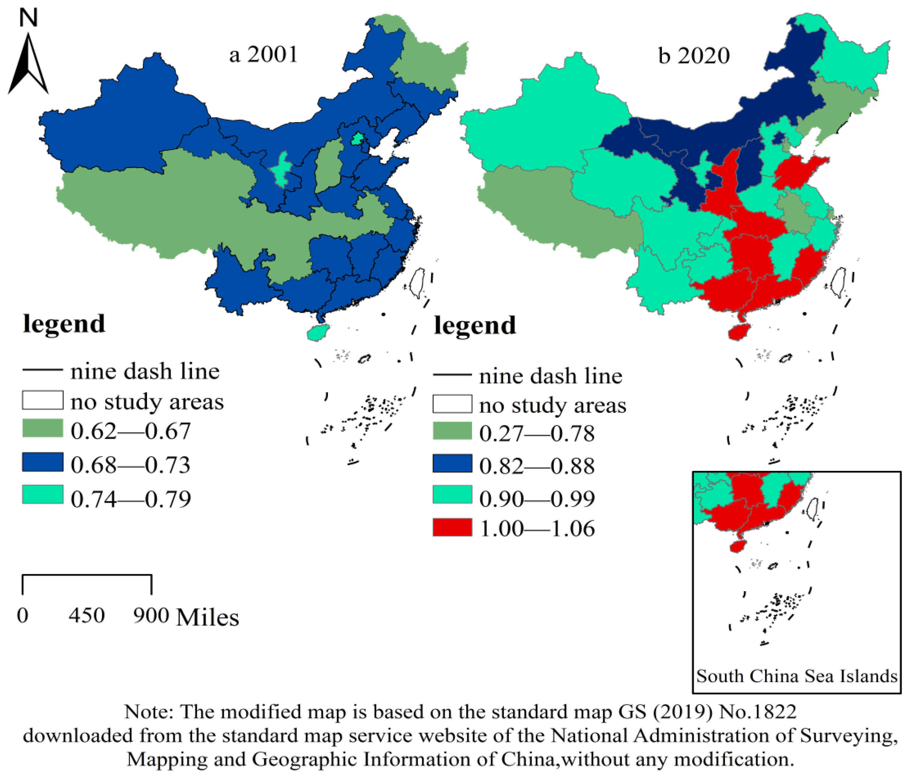
3.2. Spatial-Temporal Evolution Characteristics of Agricultural Green Development

To identify the variations of agricultural green development between the years 2000 to 2020 more directly (Given 2000 is selected as the base period of agricultural green development), the spatial distribution map of agricultural green development level in 2001 and 2020 are drawn based on the SBM-GML index and the natural fracture method of ArcGIS10.8 software (Shown in Figure 3).
Figure 3 shows that there are differences in the level of agricultural green development among provinces, and the overall agricultural green development has increased. In terms of time, the maximum value of agricultural green development varied from 0.79 to 1.06 from the years 2001 and 2020. Moreover, the number of provinces with high-levels of agricultural green development has increased, which shows a gradual trend for the better. The lowest level of agricultural green development was 0.62 in Shanxi Province in 2001, which may focus on the coal industry, and the highest level was 1.06 in Shaanxi Province in 2020, while Shanghai has the lowest level (0.27.The reason maybe that Shanghaitend to invest in secondary and tertiary industries [41].
From the spatial perspective, the level of agricultural green development is high in the east and low in the west; this may be because the eastern region has a good endowment of agricultural resources, while the southwestern region has poor natural conditions and a fragile ecological environment. In general, the level of agricultural green development has steadily improved in the whole country. Regions with high levels of agricultural green development could play a radiative driving role, and each province would complement and compensate others in resources and technologies in the process of promoting agricultural green development.

3.3. Spatial Dubin Model Regression Analysis

On the basis of the above spatial Dubin model, this paper uses Stata16.0 software for empirical estimation. Table 4 shows the regression results of environmental regulation and financial support for agriculture on agricultural green development from Model 4 to Model 7.
According to the results of model 4 and model 5 in Table 4, both the regression coefficient and the spatial lag term of environmental regulation are negative. The spatial lag term is significant at the level of 1%, which supports H1. The reason is that although the government has invested much manpower, materials and governance costs to protect the environment, it has not reversed negative externalities of environmental governance as agricultural operators need to invest more cost to meet the requirements of environmental regulation. Thus, there is an asymmetry between the benefit and costs of agricultural operators, which leads to their unwillingness to agricultural green development [42,43].
Financial support for agriculture has a significant positive effect on agricultural green development, which supports H2. This is mainly because local governments have strong autonomy and a considerable amount of financial support for agriculture, which promotes agricultural green development. However, the interaction term between environmental regulation and financial support for agriculture has a negative impact on agricultural green development, which supports H3. This is because, on the one hand, under the existing local interest incentive system, local governments are more willing to offer economic support while ignoring the reasonable use of environmental regulation means, which leads to poor environmental awareness and low attention to the agricultural environment of agricultural operators. On the other hand, under high environmental pressure, the local government might overuse environmental regulation, which leads to the cost increase of agricultural green development of agricultural operators and lowers their willingness [44].
According to model 6 and model 7 in Table 4, the variable of a spatial lag term is significant, indicating that there is a spatial spillover effect of agricultural green development. Compared with the static panel model, the dynamic panel model considering the first-order lag term of agricultural green development has a better fit, and the coefficient sign of the estimated results is consistent with the significance, which has better stability. That means there is a significant time lag effect and space spillover effect of agricultural green development. Moreover, the results show that agricultural green development has a strong dependence on the time dimension, and the level of agricultural green development in the previous period would also affect the accumulation of agricultural green development in the next period.
The estimated coefficients of environmental regulation and financial support for agriculture are in the same direction as those of the static panel model. However, the negative inhibitory effect of environmental regulation is gradually decreased, while the positive promoting effect of financial support for agriculture is constantly enhanced. This is because the local government would also increase taxes on non-agricultural sectors while providing subsidies to agricultural sectors and regulating the agricultural environment by means of incentive environmental regulation, which is similar to the find of Guo et al. [36]. Moreover, the coefficient of the interaction term between environmental regulation and financial support for agriculture varies from the range of −0.12 and −0.13 in the static panel model, indicating that the dynamic panel model could effectively reduce the bias of the regression coefficient, which is an optimized model compared with the static panel model.
In view of control variables, the results of Table 4 show that industrial structure has positive effect on local agricultural green development, while shows spatial negative spillover effect on adjacent agricultural green development. The reason may be that different provinces have a different mode of agriculture industry structure, and the agricultural industry structure efficiency shows overlapping among regions resulting in negative spillover effect with adjacent regions [40]. However, there is a significant positive spillover effect of labors’ education level on agricultural green development, and the influence coefficient shows a stable and increasing trend, indicating that labor producers with high education levels have a strong awareness of agricultural environmental protection and tend to adopt green production technology [45].

3.4. Spatial Spillover Effect Decomposition

A Dubin model could show the influence of environmental regulation and financial support for agriculture on the agricultural green development. However, it cannot accurately forecast the influence. Thus, further calculation of a partial differential equation is required, in which the total effect is decomposed into direct and indirect effect; thus, the comprehensive environmental regulation and financial support for agriculture on agricultural green development is discussed. The influences of specific decomposition are shown in Table 5.
According to the decomposition results of the spatial Dubin model effect shown in Table 5, the direct effect, spatial effect and total effect of environmental regulation on agricultural green development are all significantly negative, indicating that the greater the environmental regulation, the lower the level of agricultural green development, which is both supported in local and adjacent regions. Conversely, the direct effect, spatial effect and total effect of financial support for agriculture on agricultural green development are all significantly positive, indicating that the greater the financial support for agriculture, the higher the level of agricultural green development in both local and adjacent regions. Furthermore, the spatial interaction spillover effects between environmental regulation and financial support for agriculture on agricultural green development is significantly negative, while the coefficient decreases gradually. Agricultural green development would decrease by 0.17% when the interaction term between environmental regulation and financial support for agriculture decreases by 1%, among which the direct effect is −0.01% and the indirect effect is −0.16%. Additionally, the total effects of industrial structure on agricultural green development are lower than that of direct effect and spatial spillover effect. In contrast, the direct effect of workers’ education on agricultural green development is lower than that of the spatial spillover effect and the total effect.

3.5. Heterogeneity Analysis

3.5.1. Stage Heterogeneity Analysis

The previous research shows that agricultural green development is a gradual process. As such, this paper refers to relevant research [45] and divides the developing process of agricultural green development into two stages. The first stage is between the years 2000–2014, which is the initial construction stage of supporting a policy system for agricultural green development, focusing on quality and promoting agriculture. The second stage is between the years 2015–2020, which is the systematic stage of supporting the policy system for agricultural green development, focusing on promoting agriculture green development through high-quality inputs and outputs in the years 2015–2020.

3.5.2. Regional Heterogeneity Analysis

As previous research generally divided samples into the east, central and west regions with regional heterogeneity analysis, which would cut off the connection between adjacent provinces in the same region. Therefore, this paper refers to relevant research [46] and divides the samples into the east-central region, east-west region and middle-west region for further search, the results are shown in Table 6.
From the result of stage heterogeneity analysis in Table 6, it is seen that the spatial spillover effect on the systematic stage of agricultural green development in the years 2015–2020 is obviously more significant than that in the initial stage of agricultural green development in the years 2000–2014, and the influence coefficient is lager, indicating that agricultural green development has experienced a process of continuous improvement. Furthermore, the coefficient of financial support for agriculture on agricultural green development increases from 0.78 to 3.39. In contrast, the coefficient of environmental regulation on agricultural green development decreases from −0.005 to −0.127. Additionally, the negative coefficient of the interaction term between environmental regulation and financial support for agriculture on agricultural green development shows a shrinking trend, indicating that local government constantly adjusts the intensity of environmental regulation and financial support for agriculture according to their local situation to meet the requirements of agricultural green development.
From the perspective of spatial characteristics, there are significant differences in environmental regulation and financial support for agriculture among the east-middle region, east-west region and middle-west region. Financial support for agriculture could significantly promote agricultural green development with a spatial spillover effect in the east-middle region and east-west region while showing no significant effect in the middle-west. This may be due to the fact that the economic and technological development in the eastern region is more advanced, and its spillover effect on the central and western regions is more significant. However, environmental regulation shows no spatial spillover effects on agricultural green development in the east-middle region, east-west region and middle-west region. Furthermore, the interaction term between environmental regulation and financial support for agriculture on agricultural green development shows significance only in the east-middle region.

3.6. Robustness Test

Considering the comparability of estimation results and the reliability of conclusion, this paper adopts three methods to conduct the robustness test, and the results are shown in Table 7.

3.6.1. Replace the Spatial Weight Matrix

Compared with the geographical adjacency matrix, the inverse distance spatial weight matrix could measure the relationship between farther spatial units. Thus, this paper adopts the inverse of the center geographical distance between two provinces.   d i j   represents the geographical distance between two provinces measured by latitude and longitude. The setting matrix is as follows:
  W i j = { 1 d ij , i j 0 , i = j  
The estimation results show no change in significance and directionality, indicating that the research results are robust and credible from the perspective of replacing the spatial weights.

3.6.2. Change Estimation Method

To alleviate the estimation errors caused by bidirectional causality and legacy variables and overcome the inconsistency of estimators in maximum likelihood estimation, the generalized spatial two-stage least squares method (GS2SLS) is applied in this paper. Explanatory variables and their spatial lag terms are taken as instrumental variables to alleviate the endogeneity problem as far as possible [46]. The estimation result shows no change substantially, indicating that the results of this paper are robust.

3.6.3. Adding Control Variables

The agricultural technology level could promote the efficiency of agricultural production. Therefore, this paper refers to the relevant literature and adopts the proportion of agricultural R&D of expenditure in the GDP to measure the level of agricultural technology ( tech ) [15,47]. The estimation results only show little change of coefficient, indicating that the above verification results are credible.

4. Conclusions

From the perspective of spatial spillover, SBM-GML is adopted to measure the level of agricultural green development based on the input and output indicators with the provincial panel data from the years 2000 to 2020 and the spatial spillover effect and heterogeneity analysis of the impact of environmental regulation and financial support for agriculture on agricultural green development are further empirically tested. The research results are summarized as follows:
First, the level of agricultural green development in China shows a rising trend year by year, which is consistent with previous research (Guo et al., 2022) [9]. Moreover, it shows spatial characteristics of high in the east and low in the west. Second, environmental regulation would inhibit agricultural green development in both local and adjacent regions, which is contrary to the impact of financial support for agriculture. However, the inhibitory effect of environmental regulation is gradually decreased, while the positive effect of financial support for agriculture is constantly increased with time. Third, the dual effect of environmental regulation and financial support for agriculture shows a negative spatial spillover effect on agricultural green development, while the significance coefficient shows a decreasing trend. Fourth, with the continuous improvement of the systemization of agricultural green development, the impact of environmental regulation and financial support for agriculture on agricultural green development is increasingly enhanced. Meanwhile, the spatial spillover effect is the most significant in the east-middle region while insignificant in the east-west region and west-middle region, which is consistent with the research of Liu et al. [46].

5. Discussion

China’s agricultural production has increasingly relied on chemical fertilizers, pesticides, plastic film and other modern means [48], which resulted in greatly improved efficiency of agricultural production while sacrificing agricultural ecological environment [49], such as polluted rural water and soil [50]. As such, China attaches great importance to agricultural green development and achieving the target of agricultural carbon peaking and carbon neutrality strategy. Therefore, by clarifying the influencing mechanism of financial support for agriculture and environmental regulation on agricultural green development, the current policy requires to be strengthened from the following aspects.
First, a variety of environmental regulation means should be muti-adopted to reduce the cost of agricultural green development caused by command environmental regulation, such as the combination of incentive and punishment environmental regulation.
Second, financial support for agriculture should be strengthened, and the effect of financial support on agricultural green development should be monitored. In addition, transfer payments should be made full use to strengthen financial support for agriculture in areas which are with a weak foundation for agricultural green development.
Third, policies related to environmental regulation and financial support for agriculture should be integrated into strategies for agricultural carbon peaking and carbon neutrality, as well as medium-and long-term plans for sustainable agricultural development. Meanwhile, the assessment targets for financial subsidies and environmental supervision should be changed to link with agricultural green innovation and the quality of green agricultural products.
Fourth, the spatial spillover effect should be further explored to narrow the inter-provincial gap in agricultural green development. The east and middle region should not only maintain the comprehensive advantages of financial support for agriculture and environmental regulation but also play a demonstrative role and spread their advantages of talents and technology to the middle and west regions to achieve coordinated development of China.
In addition, it is also necessary to further improve the utilization efficiency of agriculture-related funds, strengthen the critical investment and supervision of financial support for agriculture funds, promote supervision and assessment and local government’s responsibility, as well as improve the incentive and restraint mechanism linking the effectiveness of ecological protection for the allocation of funds.

Author Contributions

Conceptualization, J.J. and L.X.; methodology, J.J.; software, J.J.; validation, J.J., L.X. and J.D.; formal analysis, J.J.; J.J. and L.X. conceived and designed the research question. J.J. constructed the models and wrote the paper. J.D. reviewed and edited the manuscript. All authors have read and agreed to the published version of the manuscript.

Funding

This research was funded by the National Natural Science Foundation of China (No. 72174076; 71704066, 72174054, and 71704068); National Social Science Foundation of China (No. 22AGL028 and 20BGL191), Social Science Foundation of Jiangsu Province (No. 21GLB016 and 22GLA007), Special research project of think-tanks in Grand Canal Cultural Belt Construction Research Institute (No. DYH21YB08).

Institutional Review Board Statement

Not applicable.

Informed Consent Statement

Not applicable.

Data Availability Statement

The data presented in this study are available within the article.

Acknowledgments

The authors are grateful to the anonymous referees who provided valuable comments and suggestions to significantly improve the quality of the paper.

Conflicts of Interest

The authors declare no conflict of interest.

References

  1. Jiang, G. How does Agro-Tourism Integration Influence the Rebound Effect of China’s Agricultural Eco-Efficiency? An Economic Development Perspective. Front. Environ. Sci. 2022, 10, 921103. [Google Scholar] [CrossRef]
  2. Wang, H.; Wang, X.; Sarkar, A.; Zhang, F. How Capital Endowment and Ecological Cognition Affect Environment-Friendly Technology Adoption: A Case of Apple Farmers of Shandong Province, China. Int. J. Environ. Res. Public Health 2021, 18, 7571. [Google Scholar] [CrossRef] [PubMed]
  3. Mazur, K.; Tomashuk, I. Governance and Regulation as An Indispensable Condition for Developing the Potential of Rural. Areas. Balt. J. Econ. 2019, 5, 67–78. [Google Scholar] [CrossRef]
  4. Hou, D.; Wang, X. Inhibition or Promotion?—The Effect of Agricultural Insurance on Agricultural Green Development. Front. Public Health 2022, 10, 910534. [Google Scholar] [CrossRef] [PubMed]
  5. Guo, L.; Guo, S.; Tang, M.; Su, M.; Li, H. Financial Support for Agriculture, Chemical Fertilizer Use, and Carbon Emissions from Agriculture Production in China. Int. J. Environ. Res. Public Health 2022, 19, 7155. [Google Scholar] [CrossRef]
  6. Nowak, A.; Kasztelan, A. Economic Competitiveness vs. Green Competitiveness of Agriculture in the European Union Countries. Oeconomia Copernic. 2022, 13, 379–405. [Google Scholar] [CrossRef]
  7. Li, Y.; Huang, L. Fiscal Spending on Environmental Protection on Carbon Emission Reduction of Spatial Spillover Effect Analysis. J. Statis. Decis. 2022, 38, 154–158. [Google Scholar] [CrossRef]
  8. Gao, Y.; Tao, W.; Wen, Y.; Wang, X. A Spatial Econometric Study on Effects of Fiscal and Financial Supports for Agriculture in China. Agr. Econ. 2013, 59, 315–332. [Google Scholar] [CrossRef]
  9. Guo, H.; Li, S. Environment Regulation, Space Effect and Green Agricultural Development. J. Res. Develop. Manag. 2022, 34, 54–67. [Google Scholar] [CrossRef]
  10. Zhou, J. Analysis and Countermeasures of Green Finance Development under Carbon Peaking and Carbon Neutrality Goals. Open J. Soc. Sci 2022, 10, 147–154. [Google Scholar] [CrossRef]
  11. Zhllima, E.; Shahu, E.; Xhoxhi, O.; Gjika, I. Understanding Farmers’ Intentions to Adopt Organic Farming in Albania. New Medit 2021, 20, 97–111. [Google Scholar] [CrossRef]
  12. Ahmed, Z.; Ahmad, M.; Rjoub, H.; Kalugina, O.; Hussain, N. Economic Growth, Renewable Energy Consumption, and Ecological Footprint: Exploring the Role of Environmental Regulations and Democracy in Sustainable Development. Sustain. Dev. 2022, 30, 595–605. [Google Scholar] [CrossRef]
  13. Chen, Q.; Mao, Y.; Morrison, A. Impacts of Environmental Regulations on Tourism Carbon Emissions. J. Environ. Res. Public Health 2022, 18, 12850. [Google Scholar] [CrossRef]
  14. Shi, F.; Ding, R.; Li, H.; Hao, S. Environmental Regulation, Digital Financial Inclusion, and Environmental Pollution: An Empirical Study Based on the Spatial Spillover Effect and Panel Threshold Effect. Sustainability 2022, 14, 6869. [Google Scholar] [CrossRef]
  15. Zhang, F.; Wang, F.; Hao, R.; Wu, L. Agricultural Science and Technology Innovation, Spatial Spillover and Agricultural Green Development-Taking 30 Provinces in China as the Research Object. Appl. Sci. 2022, 12, 845. [Google Scholar] [CrossRef]
  16. Tang, H.; Tie, W.; Zhong, F. Research on the Spatial Spillover Effect of Environment Government in China. Stat. Inf. Forum. 2022, 37, 75–89. [Google Scholar]
  17. Liang, L.; Qu, F.; Feng, S. Measurement of Agricultural Technical Efficiency Based on Environmental Pollution Constraints. J. Nat. Res. 2012, 27, 1580–1589. [Google Scholar]
  18. Ikram, M.; Sroufe, R.; Awan, U.; Abid, N. Enabling Progress in Developing Economies: A Novel hybrid Decision-making Model for Green Technology Planning. Sustainability 2021, 14, 258. [Google Scholar] [CrossRef]
  19. Pan, D. Research on Agricultural Productivity in China Considering Resources and Environment Factors; Nanjing Agricultural University: Nanjing, China, 2012. [Google Scholar]
  20. Li, C.; Chandio, A.; He, G. Dual Performance of Environmental Regulation on Economic and Environmental Development: Evidence from China. Environ. Sci. Pollut. Res. 2021, 29, 3116–3130. [Google Scholar] [CrossRef]
  21. Hamman, E.; Deane, F.; Kennedy, A.; Huggins, A.; Nay, Z. Environmental Regulation of Agriculture in Federal Systems of Government: The Case of Australia. Agronomy 2021, 11, 1478. [Google Scholar] [CrossRef]
  22. Teff-Seker, Y.; Segre, H.; Eizenberg, E.; Orenstein, D.; Shwartz, A. Factors Influencing Farmer and Resident Willingness to Adopt an Agri-environmental Scheme in Israe. J. Environ. Manag. 2022, 302, 114066. [Google Scholar] [CrossRef]
  23. Yan, C.; Yin, L.; He, B. Logistics Industry Agglomeration, Spatial Spillover Effect and Agricultural Green Total Factor Productivity: An Empirical Analysis Based on Provincial Data. China Circulat. Econ. 2022, 4, 3–16. [Google Scholar]
  24. Yan, L.; Liu, H.; Deng, Y.; Qu, Z. Agricultural Ecological Level of Capital Investment and its Spatial Spillover Effect Research. J. China Univ. Geosci. 2021, 21, 77–90. [Google Scholar]
  25. Din, S.; Erilli, N. Spatial Analysis of Determinants Affecting the Total Number of COVID-19 Cases of Provinces in Turkey. Appl. Econom. 2022, 65, 102–116. [Google Scholar]
  26. Wang, R.; He, Z. Exploring the Impact of “Double Cycle” and Industrial Upgrading on Sustainable High-quality Economic Development: Application of Spatial and Mediation Models. Sustainability 2022, 14, 2432. [Google Scholar] [CrossRef]
  27. Fang, L.; Hu, R.; Mao, H.; Chen, S. How Crop Insurance Influences Agricultural Green Total Factor Productivity: Evidence from Chinese Farmers. J. Clean. Prod. 2021, 321, 128977. [Google Scholar] [CrossRef]
  28. Li, H.; Zhou, X.; Tang, M.; Guo, L. Impact of Population Aging and Renewable Energy Consumption on Agricultural Green Total Factor Productivity in Rural China: Evidence from Panel VAR Approach. Agriculture 2022, 12, 715. [Google Scholar] [CrossRef]
  29. Chi, M.; Guo, Q.; Mi, L.; Wang, G.; Song, W. Spatial Distribution of Agricultural Eco-Efficiency and Agriculture High-Quality Development in China. Land 2022, 11, 5. [Google Scholar] [CrossRef]
  30. Qiu, W.; Zhong, Z.; Li, Z. Agricultural Non-point Source Pollution in China: Evaluation, Convergence Characteristics and Spatial Effects. Chin. Geogr. Sci. 2021, 31, 571–584. [Google Scholar] [CrossRef]
  31. Ge, P.; Wang, S.; Huang, X. Calculation of Green Total Factor Productivity of China’s Agriculture China Population. Resour. Environ. 2018, 28, 66–74. [Google Scholar]
  32. Chen, X.; Meng, Q.; Shi, J.; Liu, Y.; Sun, J.; Shen, W. Regional Differences and Convergence of Carbon Emissions Intensity in Cities along the Yellow River Basin in China. Land 2022, 11, 1042. [Google Scholar] [CrossRef]
  33. Shen, Z.; Balezentis, T.; Chen, X.; Valdmanis, V. Green Growth and Structural Change in Chinese Agricultural Sector during 1997–2014. Chin. Econ. Rev. 2018, 51, 83–96. [Google Scholar] [CrossRef]
  34. Zhan, J.; Xu, Y. Environmental Regulation, Agricultural Green Productivity and Food Security. Chin. Popul. Res. Environ. 2019, 29, 167–176. [Google Scholar]
  35. Tang, L.; Sun, S. Fiscal Incentives, Financial Support for Agriculture, and Urban-rural Inequality. Inter. Rev. Fin. Anal. 2022, 80, 102057. [Google Scholar] [CrossRef]
  36. Zhang, J.; Song, J. Analysis of the Threshold Effect of Agricultural Industrial Agglomeration and Industrial Structure Upgrading on Sustainable Agricultural Development in China. J. Clean. Prod. 2022, 341, 130818. [Google Scholar] [CrossRef]
  37. Xu, P.; Jin, Z.; Ye, X.; Wang, C. Efficiency Measurement and Spatial Spillover Effect of Green Agricultural Development in China. Front. Environ. Sci. 2022, 10, 909321. [Google Scholar] [CrossRef]
  38. Liu, J.; Zhao, M.; Wang, B. Impacts of Government Subsidies and Environmental Regulations on Green Process Innovation: A Nonlinear Approach. Tech. Soc. 2019, 63, 101417. [Google Scholar] [CrossRef]
  39. Guo, X.; Li, B.; Jiang, S.; Nie, Y. Can Increasing Scale Efficiency Curb Agricultural Nonpoint Source Pollution? Int. J. Environ. Res. Pub. 2021, 18, 8798. [Google Scholar] [CrossRef]
  40. Gao, Y.; Niu, Z. Agricultural Informatization, Spatial Spillover Effect and Agricultural Green Total Factor Productivity: Based on SBM-ML Index Method and Spatial Dubin Model. Stat. Inf. Forum. 2018, 33, 66–75. [Google Scholar]
  41. Luo, N.; Wang, Y. Fiscal Decentralization, Environmental Regulation and Regional Eco-efficiency study based on Dynamic Spatial environment. China Popul. Res. Environ. 2017, 27, 110–118. [Google Scholar]
  42. Chang, H.; Sigman, H.; Traub, L. Endogenous Decentralization in Federal Environmental Policies. Int. Rev. Law Econ. 2014, 37, 39–50. [Google Scholar] [CrossRef] [Green Version]
  43. Xia, X.; Ruan, J. Analyzing Barriers for Developing a Sustainable Circular Economy in Agriculture in China Using Grey-DEMATEL Approach. Sustainability 2020, 12, 6358. [Google Scholar] [CrossRef]
  44. Deng, H.; Jing, X.; Shen, Z. Internet Technology and Green Productivity in Agriculture. Environ. Sci. Pollut. Res. 2022, 29, 81441–81451. [Google Scholar] [CrossRef] [PubMed]
  45. Li, X.; Gong, Q. Evolution and Optimization of Agricultural Green Development Support Policies Since the Founding of New China. World Agric. 2020, 40–50. [Google Scholar] [CrossRef]
  46. Liu, Z.; Yang, Y.; Sui, X. Internet Development, Market Dynamism and Tourism Economic Growth: An Analysis from the Perspective of Spatial Spillover. Tour. Sci. 2022, 36, 14–43. [Google Scholar]
  47. Zhao, L.; Zhang, Y.; Pan, F. Environmental Regulation and Innovation Efficiency of Agricultural Science and Technology. Res. Manag. 2019, 40, 76–85. [Google Scholar]
  48. Grigoryeva, M.; Dmitrevskaya, I.; Belopukhov, S.; Osipova, A. The Chemical Training of Agrarian Specialists: From the Chemicalization of Agriculture to Green Technologies. Sustainability 2022, 14, 8062. [Google Scholar] [CrossRef]
  49. Geng, R.; Sharpley, A.N. A novel spatial optimization model for achieve the trad-offs placement of best management practices for agricultural non-point source pollution control at multi-spatial scales. J. Clean. Prod. 2019, 234, 1023–1032. [Google Scholar] [CrossRef]
  50. Lu, H.; Xie, H. Impact of changes in labor resources and transfers of land use rights on agricultural non-point source pollution in Jiangsu Province, China. J. Environ. Manag. 2018, 207, 134–140. [Google Scholar] [CrossRef]
Figure 1. Moran’s I index test results.
Applsci 12 11609 g001
Figure 2. The partial Moran’ I of environmental regulation, financial support for agriculture and agricultural green development in 2020.
Applsci 12 11609 g002
Figure 3. Spatial-temporal evolution characteristics of agricultural green development.
Applsci 12 11609 g003
Table 1. Comparison of spatial panel model test results.
Statistic of TestStatisticStatistic of TestStatistic
Moran’s I5.855 ***LR-error18.85 ***
LM (error)624.921 ***Wald-lag187.90 ***
R-LM (error)185.436 ***Wald-error135.02 ***
LM (lag)499.218 ***Individual effect294.80 ***
R-LM (lag)59.732 ***Time effect412.46 ***
LR-lag19.76 ***Hausman inspection14.14 **
Note: *** p < 0.01, ** p < 0.05.
Table 2. Connotation of input and output variables.
Variable CategoriesVariables: Definitions/UnitVariable AbbreviationsThe Data Source
InputLabor force: Number of primary industry employees/ten thousandLChina Statistical Yearbook, Statistical Yearbook of Provinces and Cities
Land resources: total sown area of crops/1000 ha, aquaculture area/1000 haBChina Rural Statistical Year-book, China Statistical Year-book
Water Resources: Total agricultural water use
(billion m3)
RChina Statistical Yearbook
Desired outputAdded value of the primary industry/100 million yuanGDPChina Statistical Yearbook
Undesired outputAgricultural carbon emissionsCO2Calculation results according to the above method
Table 3. Descriptive statistics of variables.
VariablesObsMeanStd. DevMinMax
lnagtfp6511.0390.7310−0.07873.1262
lner651−2.13651.2424−9.11452.8403
lnfiscal6515.02041.35961.55647.1999
lnstruc6512.25350.8668−1.20395.1590
lnagrimech6511.37191.5851−4.58594.5726
lnedu6511.97970.16610.80472.6071
lnscale651−1.53080.5288−3.3354−0.6005
Note: The results are based on Stata software with authors.
Table 4. The results of spatial Dubin model regression.
VariablesStatic Dubin Model
Model (4)
Static Dubin Mode
of Interaction
Model (5)
Dynamic
Dubin Model
Model (6)
Dynamic
Dubin Model
of Interaction
Model (7)
L.lnagtfp 0.1912 *
(1.90)
0.1723 *
(1.71)
lner−0.0780 ***
(−5.58)
−0.0786 ***
(−5.58)
−0.0719 *
(−5.12)
−0.0720 ***
(−5.08)
lnfiscal0.2001
(1.27)
0.2524
(1.42)
0.1580 ***
(0.97)
0.1738
(0.94)
lner × lnfiscal −0.0232
(−0.58)
−0.0052
(−0.13)
lnstruc0.2806 ***
(8.82)
0.2776 ***
(8.74)
0.2881 ***
(8.59)
0.2846 ***
(8.50)
lnagrimech−0.0146
(−1.17)
−0.0138
(−1.11)
−0.0118
(−0.90)
−0.0111
(−0.85)
lnedu−0.1742 *
(−1.66)
−0.1572
(−1.47)
−0.0396
(−0.34)
−0.0316
(−0.27)
lnscale0.0059
(0.10)
0.0032
(0.05)
0.0133
(0.21)
0.0106
(0.17)
W*lner−0.0919 ***
(−2.60)
−0.0935 ***
(−2.65)
−0.0628 *
(−1.71)
−0.0673 **
(−1.84)
W*lnfiscal1.1103 ***
(3.61)
1.4735 ***
(3.94)
1.2089 ***
(3.83)
1.6199 ***
(4.20)
W*lner × lnfiscal −0.1266 *
(−1.69)
−0.1393 *
(0.85)
W*lnstruc−0.2389 ***
(−3.41)
−0.2253 ***
(−3.21)
−0.3069 ***
(−4.15)
−0.2908 ***
(−3.91)
W*lnagrimech0.0217
(0.96)
0.0232
(1.03)
0.0163
(0.69)
0.0177
(0.75)
W*lnedu0.4119 **
(1.94)
0.4656 **
(2.17)
0.6944 ***
(2.86)
0.7473 ***
(3.07)
W*lnscale0.0507
(0.43)
0.0407
(0.34)
0.0060
(0.05)
−0.0055
(−0.44)
Log-L−2859.27−2859.27−580.44−533.07
ρ0.1907 ***
(3.62)
0.1823 ***
(3.46)
0.1341 **
(2.10)
0.1335 **
(2.09)
R20.36380.39650.59320.5838
N651651620620
Control variables and
spatial terms
YESYESYESYES
Individual fixed effectsYESYESYESYES
Time fixed effectYESYESYESYES
Note: Standard errors in parentheses, *** p < 0.01, ** p < 0.05, * p < 0.1.
Table 5. The results of spatial Dubin model of spatial spillover decomposition.
VariablesStatic of Dubin Model
Long-Term EffectsLong-Term Effects of Interaction Relationship
Direct EffectIndirect EffectTotal EffectDirect EffectIndirect EffectTotal Effect
lner−0.0822 ***
(−5.57)
−0.1255 ***
(−2.91)
−0.2077 ***
(−4.12)
−0.0828 ***
(−5.60)
−0.1275 ***
(−3.33)
−0.2104 ***
(−4.69)
lnfiscal0.2459
(1.60)
1.3430 ***
(3.70)
1.5889 ***
(3.82)
0.3118 **
(1.83)
1.8113 ***
(4.28)
2.1231 ***
(4.53)
lner × lnfiscal −0.0280
(−0.69)
−0.1546*
(−1.76)
−0.1826 *
(−1.87)
lnstruc0.2755 ***
(8.93)
−0.2132 ***
(−2.63)
0.0622
(0.69)
0.2733 ***
(8.98)
−0.2021 **
(−2.47)
0.0711
(0.79)
lnagrimech−0.0138
(−1.14)
0.0226
(0.85)
0.0087
(0.30)
−0.1312
(−1.09)
0.0221
(0.88)
0.0090
(0.33)
lnedu−0.1544
(−1.44)
0.4499 *
(1.69)
0.2955
(0.90)
−0.1357
(−1.26)
0.5352 **
(1.98)
0.3995
(1.23)
lnscale0.0129
(0.21)
0.0721
(0.50)
0.0851
(0.53)
0.0088
(0.14)
0.0398
(−1.76)
0.4868
(0.33)
VariableDynamic Dubin Model
Long-Term EffectsLong-Term Effects of Interaction Relationship
Direct EffectIndirect EffectDirect EffectIndirect EffectDirect EffectIndirect Effect
lner−0.0799 ***
(−5.47)
−0.1224 **
(−2.35)
−0.2024 ***
(−3.37)
−0.0794 ***
(−5.39)
−0.1178 **
(−0.26)
−0.1972 ***
(−3.28)
lnfiscal0.2851 *
(1.74)
1.8118 ***
(3.93)
2.0970 ***
(3.89)
0.3289 *
(1.80)
2.3221 ***
(3.97)
2.6510 ***
(4.05)
lner × lnfiscal −0.0207
(−0.53)
−0.2006 **
(−1.97)
−0.2214 *
(−1.95)
lnstruc0.2698 ***
(8.11)
−0.2973 ***
(−2.79)
−0.0274
(−0.23)
0.2676 ***
(0.81)
−0.2857 ***
(−2.95)
−0.0180
(−0.17)
lnagrimech−0.0109
(−0.85)
0.0154
(0.47)
0.0044
(0.12)
−0.0099
(−0.78)
0.0219
(0.64)
0.0119
(0.31)
lnedu0.0256
(0.20)
0.9742 **
(2.57)
0.9998 **
(2.15)
0.0335
(0.26)
0.9961 ***
(2.69)
1.0296 **
(2.23)
lnscale0.0123
(0.19)
−0.0025
(−0.01)
0.0097
(0.05)
0.0097
(0.15)
−0.0040
(−0.02)
0.0056
(0.03)
Note: Standard errors in parentheses, *** p < 0.01, ** p < 0.05, * p < 0.1.
Table 6. Analysis of heterogeneity.
VariablesStage Heterogeneity AnalysisRegional Heterogeneity Analysis
2000–2014
Early Stage
2015–2020
Systematize Stage
East-MiddleEast-WestMiddle-West
L.lngtfp0.1233
(1.17)
0.6049 ***
(2.87)
0.3720 ***
(3.02)
0.0826
(0.75)
0.1439
(0.12)
W*lner−0.0053
(−0.16)
−0.1274 **
(−2.19)
−0.0092
(−2.05)
−0.0441
(−1.18)
−0.0398
(−0.99)
W*lnfiscal0.7801 **
(2.52)
3.3919 ***
(2.16)
1.5725 ***
(3.12)
1.0188 ***
(2.63)
0.3726
(0.61)
W*lner × lnfiscal−0.0422
(−0.58)
−0.7482 *
(−1.79)
−0.3354 **
(−2.31)
−0.0977
(−1.32)
0.0139
(0.12)
Control variablesControlControlControlControlControl
ρ0.1915 **
(2.75)
0.2438 *
(1.85)
0.1647 **
(2.36)
0.0471
(0.49)
0.0923
(1.20)
N434155380460400
Log-L−2039.9252105.59−2364.6315−2025.4008−1073.0839
R20.08570.05110.19120.28780.6239
Note: Standard errors in parentheses, *** p < 0.01, ** p < 0.05, * p < 0.1.
Table 7. The results of robustness test.
VariablesReplace the Spatial Weight MatrixChange Estimation MethodAdding Control Variables
L.lngtfp0.1912 *
(1.90)
0.0836 ***
(5.26)
0.1891 *
(1.89)
lner−0.0719 ***
(−5.12)
−0.0253 *
(−1.67)
−0.1171 ***
(−4.62)
lnfiscal0.1580
(0.97)
0.4690 *
(3.45)
0.1587
(0.98)
lnstruc0.2881 ***
(8.59)
0.1407 ***
(9.34)
0.2875 ***
(8.61)
lnagrimech−0.0118
(−0.90)
−0.0275 ***
(−2.77)
−0.0125
(−0.96)
lnedu−0.0396
(−0.34)
0.3557 ***
(4.44)
−0.0436
(−0.38)
lnscale0.0133
(0.21)
−0.1031
(−4.31)
0.0135
(0.21)
lntech 0.0458 **
(2.13)
W*lner−0.0628 *
(−1.71)
−0.0975 *
(−1.81)
W*lnfiscal1.2089 ***
(3.83)
1.1833 ***
(3.76)
W*lnstruc−0.3069 ***
(−4.12)
−0.3004 ***
(−4.08)
W*lnagrimech0.0163
(0.69)
0.0190
(−4.08)
W*lnedu0.6944 ***
(2.86)
0.6744 ***
(2.79)
W*lnscale0.0060
(0.05)
0.0353
(0.29)
W*lntech 0.0357
(0.87)
ρ0.1341 **
(2.10)
1.3020 ***
(−4.93)
0.1276
(1.99)
N620620620
Log-L−580.4485.2713−721.2347
R20.59320.91560.5685
Control variables and
spatial terms
YESYESYES
Individual fixed effectsYESYESYES
Time fixed effectYESYESYES
Note: Standard errors in parentheses, *** p < 0.01, ** p < 0.05, * p < 0.1.
Publisher’s Note: MDPI stays neutral with regard to jurisdictional claims in published maps and institutional affiliations.

