Supervised Learning Algorithm for Predicting Mortality Risk in Older Adults Using Cardiovascular Health Study Dataset

Featured Application

In this project, we designed an algorithm to predict mortality from multiple chronic conditions and cardiovascular diseases. We designed this algorithm to function as a decision aid for healthcare professionals.

Abstract

Multiple chronic conditions are an important factor influencing mortality in older adults. At the same time, cardiovascular events in older adult patients are one of the leading causes of mortality worldwide. This study aimed to design a machine learning model capable of predicting mortality risk in older adult patients with cardiovascular pathologies and multiple chronic diseases using the Cardiovascular Health Study database. The methodology for algorithm design included (i) database analysis, (ii) variable selection, (iii) feature matrix creation and data preprocessing, (iv) model training, and (v) performance analysis. The analysis and variable selection were performed through previous knowledge, correlation, and histograms to visualize the data distribution. The machine learning models selected were random forest, support vector machine, and logistic regression. The models were trained using two sets of variables. First, eight years of the data were summarized as the mode of all years per patient for each variable (123 variables). The second set of variables was obtained from the mode every three years (369 variables). The results show that the random forest trained with the second set of variables has the best performance (89% accuracy), which is better than other reported results in the literature.

1. Introduction

Multiple chronic conditions (MCC) are defined as “conditions that last a year or more and require ongoing medical attention and/or limit activities of daily living” [1]. Among the most common chronic conditions are hypertension, heart disease, cardiovascular disease, arthritis, diabetes, cancer, dementia, and various cognitive disorders. The number of people with MCC has increased over the years and, combined with aging, has become a major global health challenge [2]. Because people with MCC must frequently be hospitalized, expenses related to medical care have also risen. In addition, health services worldwide have been focusing on individual chronic diseases, so there are few projects that address the prediction of factors such as mortality from MCC. This situation makes it necessary to create a tool that can predict different factors, such as mortality, from MCC. This tool would help health professionals to make decisions and subsequently treat patients suffering from these conditions.

Not surprisingly, multiple chronic diseases and cardiovascular pathologies are associated with impaired quality of life, an increased risk of disability, institutionalization, and mortality, and higher healthcare utilization and associated costs. For example, the annual risk of hospitalization increases from 4% among individuals with zero to one chronic condition to more than 60% for those with six or more chronic conditions. Furthermore, 30-day readmission rates increase progressively as the number of chronic conditions rises, and per capita, Medicare expenditures increase exponentially as a function of the number of chronic conditions [3]. Additionally, physician care is based on treating one disease at a time and does not consider the possible effects of a combination of different pathologies.

Performing mortality prediction based on multiple chronic conditions and cardiovascular diseases can be a significant challenge for a healthcare professional. Correct prediction can identify patients with a higher risk to their health, allowing physicians to take appropriate measures to avoid or minimize this risk and, in turn, improve the quality of care and avoid potential hospital admissions [4]. The related work section shows that the use of machine learning algorithms to predict mortality and other pathologies has been increasing in recent years. This increase is because machine learning algorithms provide the tools to make an automatic and accurate mortality prediction, which is why they greatly support the decision-making process of health professionals. In addition, the literature review reveals that the most used models are those based on decision trees and support vector machines, with an increase in the use of neural networks at the present time [5].

This study aimed to predict patients’ mortality risk from cardiovascular variables, medical history, medications, and electrocardiogram variables. Supervised learning algorithms were used to perform the predictions.

Related Work

First, there will be a discussion of the main aspects and challenges of mortality risk prediction in older adult patients with multiple chronic conditions and cardiovascular pathologies. In order to predict mortality, the effect of different variables must be taken into account. Rodgers et al. conducted a study to show the association between cardiovascular risk and the age and gender of patients. This study showed that age is an important factor in the deterioration of cardiovascular function, resulting in an increased risk of cardiovascular disease (CVD) in older adults. It also showed that the prevalence of CVD increases with age in both men and women, including the prevalence of atherosclerosis, stroke, and myocardial infarction; in fact, the incidence of CVD is 89.3% in men and 91.8% in women in adults older than 80 years. Patients’ risk may change depending on other pathologies, such as diabetes, hypertension, and obesity. A high prevalence of heart failure, atrial fibrillation, and other forms of CVD was first noted in elderly patients. The high prevalence of CVD in this population has been linked to many factors, including increased oxidative stress, inflammation, apoptosis, and general myocardial deterioration and degeneration [6].

With the progress of sophisticated machine learning algorithms and advanced data collection and storage technologies, researchers have achieved promising results for predicting the risk of having a single chronic disease. State-of-the-art machine learning algorithms, such as deep neural networks, support vector machines, logistic regression, random forest, and decision trees, have been widely implemented and validated to predict the risk of having chronic diseases, such as hypertension, cardiovascular disease, heart disease, and diabetes mellitus. Much of the research has focused on predicting a single chronic disease, but chronic diseases, especially in old age, often co-occur with other chronic diseases, a phenomenon known as multimorbidity or MCC. The lack of a model for multiple chronic conditions can be attributed to the paucity of a dataset covering MCC. Available datasets are usually dedicated to a particular type of disease. To address this challenge, Yang et al. designed interpretable machine learning algorithms to tackle the problem of classifying whether or not a participant is at high risk for CCM by identifying associated risk factors and exploring the interactions between them. Yang et al. used the Catapult Health database, which consists of 451,425 records, among which 137,118 records, 77,149 records, and 237,159 records were collected in 2018, 2017, and 2012–2016, respectively. For this study, 301,631 patients were selected, of which 10,427 participants (3.5%) were flagged as high-risk individuals with at least one chronic condition, and 291,204 participants (96.5%) were flagged as low-risk individuals without CCM. Twenty variables were selected for analysis: diastolic blood pressure (DBP), systolic blood pressure (SBP), glucose (GLU), triglycerides (TGS), total cholesterol (TCHOL), body mass index (BMI), low-density lipoprotein (LDL) cholesterol, weight, age, alanine aminotransferase (ALT), blood pressure assessment, abdominal circumference, metabolic syndrome risk, diabetes assessment, and BMI assessment. Seven machine learning algorithms, namely, k-nearest neighbors (kNN), decision tree (DT), random forest (RF), gradient boosting tree (GBT), logistic regression (LR), support vector machine (SVM), and Naïve Bayes (NB), were used and evaluated for this study. Regarding the results, the AUC values achieved by the GBT classifier, RF classifier, SVM classifier, DT classifier, NB classifier, LR classifier, and kNN classifier were 0.850, 0.846, 0.833, 0.837, 0.821, 0.823, and 0.826, respectively [7].

In another study by Kawano et al., 85,361 patients were selected, and three machine learning models, XGBoost, artificial neural network, and logistic regression, were built to predict mortality based on different cardiac variables and chronic conditions. Regarding the results, the AUC values were 0.811 for XGBoost, 0.774 for neural networks, and 0.772 for logistic regression models, indicating that the predictive capacity of XGBoost was the highest. This study showed that the machine-learning-based model has a higher predictive ability than the conventional logistic regression model and can be helpful in risk assessment and health counseling for health checkup participants [8].

In order to design the algorithm, a review of previous studies was carried out to establish the main variables affecting mortality and other medical events and the algorithms and supervised learning methods used in these situations. Di Castelnuovo et al. and Mirkin et al. performed a study to identify the cardiovascular characteristics, comorbidities, and laboratory measures associated with in-hospital mortality in European countries [9,10]. The random forest model used by the authors found that among the most important variables for predicting mortality were impaired renal function, elevated C-reactive protein, advanced age, diabetes, hypertension, and myocardial infarction. Cox’s multivariate survival analysis confirmed these results. Another study by Kaiser et al. [11] used the information from 529 patients from the CHS database to describe the effect of social support on survival after heart failure. The authors built a Cox survival model using the following as variables: age, gender, race (white or black), medications (antihypertensive, oral hypoglycemic, and lipid-lowering), coronary heart disease status (defined as myocardial infarction, angina, coronary artery bypass grafting, or angioplasty), systolic and diastolic blood pressure, cystatin-C, general health status (excellent, good, fair, or poor), self-reported limitations in activities of daily living (ADLs), body mass index, and physical activity. The model results showed that participants with high scores in social networks tend to have a higher body mass index (BMI), fewer depressive symptoms, and better interpersonal support scores. Another interesting result was that participants with a high social support score had a 29% lower mortality rate than those with a low score. These findings suggest that structural social support prior to diagnosis may modestly buffer mortality in patients with heart failure. In [12,13,14], to analyze risk factors for hospital readmission, a study was conducted with 100 patients and Chi-square tests. The results showed that the most influential variables in hospital readmission were noncompliance with medication (25.8%), poor dietary compliance (22.6%), uncontrolled diabetes mellitus (22.6%), ischemia (19.4%), anemia (16.1%) and worsening left ventricular function (16.1%).

The most used supervised learning methods are decision-tree-based algorithms such as random forest, support vector machine, and Naive Bayes and survival algorithms such as Cox regression, as shown in the studies conducted by Guo et al., Segar et al., and Mezzatesta et al. [14,15,16]. The variables commonly used to train the mentioned models are demographic variables, laboratory examination data, and clinical, cardiovascular, and electrocardiogram variables. Finally, da Silva et al. [17] present a deep learning algorithm to predict the deterioration of patients’ health. This DeepSigns model predicts vital signs using LSTM networks and calculates the prognostic index for the early diagnosis of patients’ worsening health status. To construct the predictor, the authors used fifteen attributes, such as temperature, blood pressure, heart rate, oxygenation, hematocrit, and age, among others. In general, the main contributions of their work were (i) the development of a method to predict patient data, feeding back new data to the model to obtain greater accuracy, and (ii) the evaluation of many prognostic indices using predicted vital signs instead of specific values measured over time. The final model was able to predict vital signs with 80% accuracy with regard to the results obtained, identifying states of possible future deterioration. As can be seen, there are studies in the literature that used machine learning models to predict mortality based on sociodemographic and clinical variables. However, studies were not found using a cardiovascular study database (CHS) to make such associations and predictions using machine learning. Articles using similar methodology and variables but with other datasets show performance ranging from 66% to 81% [18,19,20,21].

As seen in the literature review, mortality predictions using machine learning algorithms from multiple chronic conditions, including cardiovascular and other physiological variables, have been increasing. Some of the variables used for mortality predictions have already been described, and the main algorithms used have been discussed. However, one of the main prediction challenges is to acquire suitable data. The Cardiovascular Health Study was an observational study to identify risk factors for cardiovascular disease in older adults. The results of this study are available to researchers to investigate conditions that affect older adults and constitute a valuable source for secondary use. This database provides 20 years of data for 5125 patients. This article aims to study mortality risks by relating, through machine learning models, multiple chronic conditions and other clinical variables in older adults using the CHS dataset [22].

2. Materials and Methods

2.1. Dataset: Cardiovascular Health Study (CHS)

As its dataset, this study used the Cardiovascular Health Study (CHS) available from BioLincc. The Cardiovascular Health Study (CHS) was an observational study to identify risk factors for the development and progression of cardiovascular disease (CVS) in older adults, initiated by the National Heart, Lung, and Blood Institute (NHLBI) in 1987. A total of 5201 men and women were recruited from four communities. The population from the Pittsburgh Field Center was entirely urban, and the other three Field Centers recruited a mixture of urban and rural populations. Eligible participants were sampled from Medicare eligibility lists.

The dataset includes physical and laboratory measurements at baseline with the aim of identifying the presence and severity of CVD risk factors such as hypertension, hypercholesterolemia, and glucose intolerance, subclinical diseases. The database has 5888 patients, where 5125 correspond to the first recruitment (old cohort) and 763 correspond to the second (new cohort). In the study, 3329 patients were women, while 2466 were men. Follow-up was carried out between 1989 and 1999 using the old cohort, after which the new cohort was added. After 2000, 2 calls per year continued to be made to update patient data and monitor the evolution of different cardiovascular diseases. For the study, various annual physical and laboratory evaluations were performed along with biannual telephone calls to identify the presence and severity of risk factors for cardiovascular disease [22]. During these telephone calls, patients were given questionnaires to assess the evolution of the different cardiovascular variables measured in the previous medical examinations. Some of the examinations performed on CHS patients were:

• The analysis of psychosocial factors, such as depression;
• Healthcare variables, such as medication, medical history, and hospitalizations;
• Blood pressure measurements, such as the ankle–arm ratio;
• Physical and functional examinations;
• Tests to measure neurological function;
• Electrocardiography;
• Laboratory tests;
• Lipid measurement;
• Ultrasonography;
• Echocardiography.

The cardiovascular study is the most extensive NHLBI-funded study in older adults, with ten years of clinical measurements and approximately seven years of telephone follow-up. This dataset is appropriate for secondary analyses using machine learning models that generally require an adequate number of variables and a good sample size. Because the model in this study needs variables with an adequate information density and the least number of missing values, it was decided to use ten years of data (from 1989 to 1999) to build the machine learning models after an exploratory analysis.

2.2. Prediction Models

2.2.1. Analysis and Selection of Variables

A correlation analysis determined which variables significantly influence mortality and other cardiovascular events, such as myocardial infarction. The correlation makes it possible to measure the association between two variables and the direction of this relationship. A correlation result is a number between −1 and 1. A value of ±1 indicates a perfect degree of association between the variables; if the value is 0, the relationship between variables is weak [23]. The sign of the result indicates the direction of the relationship: a positive result indicates a positive relationship between the variables; therefore, as one variable increases, so does the other. In contrast, a negative result indicates a negative relationship, so as one variable increases, the other decreases. One of the methods for calculating correlations is Spearman’s correlation, which evaluates the monotonic relationship between two continuous or ordinal variables. In a monotonic relationship, the variables change simultaneously, but not necessarily at a constant rate. Spearman’s correlation is defined by Equation (1) [23]. Based on correlation results and the analysis of previous work, 123 CHS variables were selected.

Table 1. Some of the selected variables from the CHS database.

Variable	Variable
Heart rate	Complete heart block
Injury or ischemia	Age
LV mass (gm)	Gender
Ventricular tachycardia	Smoking amount (quantity of cigarettes smoked in a week)
Chest pain	Depression scale total
Cardiac injury score	Weight in lb
Atrial flutter	Taking Medication? H-2 blockers
Atrial fibrillation	Taking Medication? Fibrates
Angina	Taking Medication? Any diuretic
Stroke	Taking Medication? Nitrates
Diabetes	Taking Medication? Any calcium channel blocker
Hematocrit (%)	Taking Medication? Progestins
Cholesterol	Taking Medication? Alpha-blockers
Systolic and diastolic pressure	Heparins
Myocardial infarction	Taking Medication? Insulins

shows the selected variables. The selected variables include electrocardiogram variables, such as times of different intervals (e.g., ST-T, QRS) and abnormalities on examination. Cardiovascular variables such as heart rate, various cardiac problems, cholesterol, hematocrit, and cardiovascular diseases (myocardial infarction, angina, and heart failure) were also selected. In addition, demographic and functional variables were selected, such as age, gender, weight, depression, smoking status, and variables of day-to-day difficulties. Finally, medication variables were selected: alpha-blockers, calcium channel blockers, nitrates, and diuretics.

$$p=1-\frac{6{{\displaystyle \sum }}_i{d}^2{}_i}{n\left(n^2-1\right)},$$

(1)

In relation to the 123 selected variables, there are electrocardiogram variables related to segment time (QRS, ST-T) and also binary variables related to abnormalities in the electrocardiograms for each patient. On the other hand, variables related to medications were of the binary type and indicated whether or not they were taking the respective medicines. Finally, the variable smoker was also selected to be part of the model. There are two variables associated with smoking patients in the dataset: (i) the number of cigarettes smoked by the patients in a given time and (ii) whether the patient was a light (<10 cigarettes/day), moderate (10–19 cigarettes/day), or heavy smoker (≥20 cigarettes/day).

2.2.2. Variable Engineering

Data preprocessing, also called variable engineering, involves various processes, including creating feature matrices to train the models, splitting the dataset into training and testing, preprocessing missing data, and variable scaling.

A.

Creation of feature matrices to train the models: For a health professional using an algorithm of this type, it is beneficial to obtain the result based on the evolution of the patients over time and not only their current state. Therefore, eight years of data were taken from the database and grouped into two matrices of different characteristics used to make the prediction.

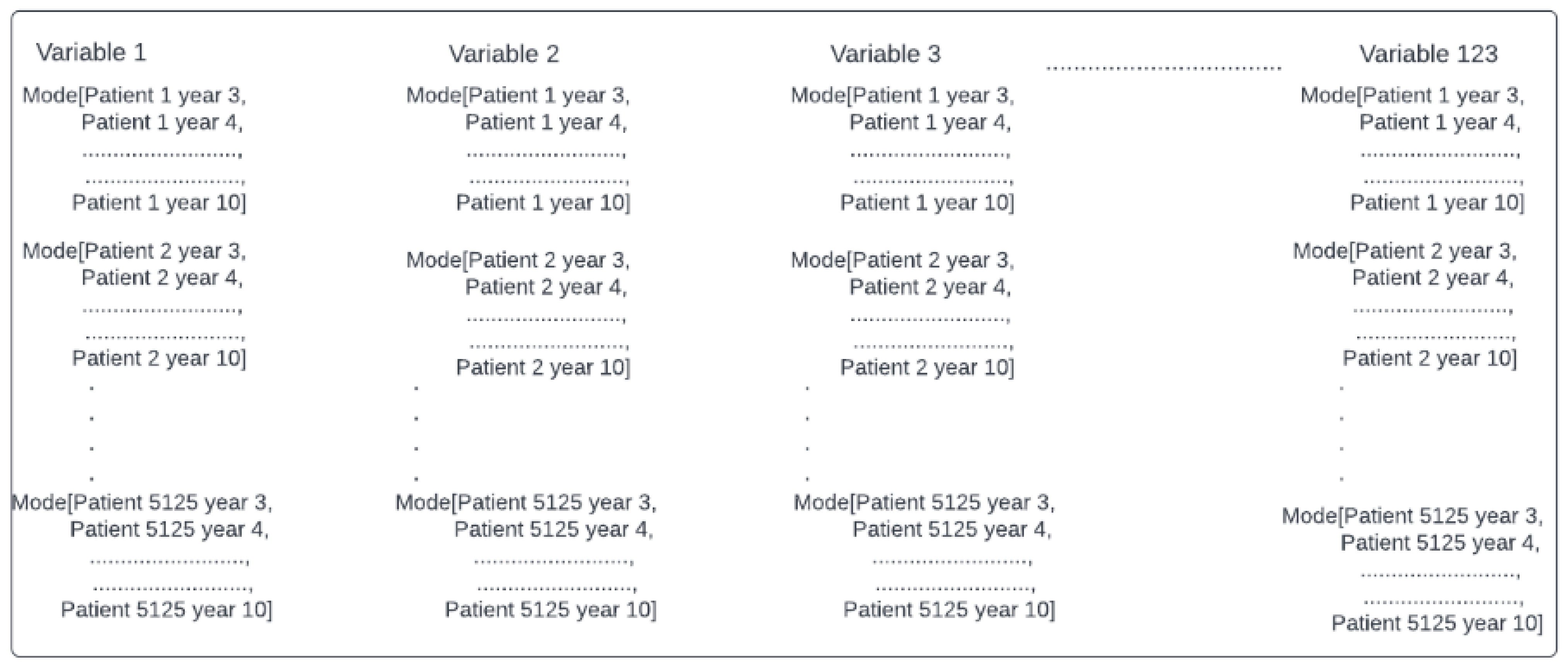
The first matrix grouped eight years of data, calculating the mode for each variable in all of those years, as shown in Figure 1, totaling 123 variables. The purpose of grouping is to obtain a value for each variable representing the results and the change in the variable itself over the eight years.

However, since the first matrix summarizes data from eight years in a particular value, a second matrix that maintained a more temporal character than the first was created. For this purpose, the eight years of data were grouped by calculating the mode every three years, as shown in Figure 2. In this way, each variable is divided into three sub-variables, and the models can better analyze the temporal change in the data. Note that both matrices have the same number of rows, but the second matrix has a more significant number of columns (349 variables in total).

B.

Splitting the dataset into training and testing: The 5125 patients were divided into training and test sets. The Pareto Principle (80/20 rule) specifies that 80% of the results are derived from 20% of the causes [24]. Thus, considering this rule and the number of patients in the database, theoretically, using 80% of the data for training purposes and 20% for testing purposes will help to avoid possible overfitting. On the other hand, if there are fewer training data, the machine learning model will show high variance in training. The model performance evaluation will have a higher variance with fewer test data. Essentially, the aim is to balance the partitioning so that the variance is minimal.

C.

Preprocessing of missing data: All selected CHS variables have a percentage of missing data. The mode of the respective column was used to replace those variables with missing values (nan) in the database.

D.

Variable scaling: Most of the variables selected are categorical (1 or 0), but other variables have higher values (such as weight, ECG times, and other tests). Therefore, the scaling of variables was performed so that all values would be between 0 and 1 [25].

2.2.3. Supervised Learning Models

The literature review states that mortality risk models are usually modeled through random forest, support vector machine, and logistic regression. These models were selected because of their implementation simplicity and lower computational resource consumption. All models were trained using the two feature matrices created earlier. The definition of the models and mode of use are shown below.

A.

Random Forest: The random forest algorithm is based on multiple decision trees. A decision tree delivers a classification result based on the properties and characteristics of the data. The most repeated result gives the result of a random forest among the trees. The RandomForestClassifier function of Scikit Learn has several parameters to perform the training, such as the number of trees (n_estimators), tree depth (max_depth), the minimum number of samples to split the internal node (min_samples_split), the minimum number of samples per leaf (min_samples_leaf), the maximum number of features (max_features), and the sample selection method for training each tree (bootstrap). The GridSearch method of Scikit Learn was used to find the optimal combination of these parameters with the best performance [26,27].

B.

Support Vector Machine: SVM is an algorithm that aims to find a hyperplane in an N-dimensional space (where N is the number of features) that classifies the data points. There can be different hyperplanes to separate two classes, but the search is for the one with the maximum margin; i.e., the distance between two points of both classes is maximum. Choosing this hyperplane generates a more reliable classifier, which behaves well in different instances. It is worth mentioning that the dimension of the plane depends on the number of input features: if there are two input features, the hyperplane will be a line, while if the dimension is increased, there will be an N-dimensional hyperplane. There are also support vectors, which are points near the hyperplane. Finding suitable support vectors helps to maximize the SVM margin. The most crucial parameter for training an SVM is the kernel. In the case of this project, a sigmoid kernel was used for all implemented SVMs. In addition, the SVC function of Scikit Learn (with gamma = “auto”) was used to train the models. [28].

C.

Logistic Regression: The logistic regression algorithm estimates the probability that an instance belongs to a particular class. If the estimated probability is greater than 50%, the model predicts that the instance belongs to that class (labeled “1”) and otherwise predicts that it does not (labeled “0”). Unlike linear regression, logistic regression uses the logistic function to make the result of a linear equation lie between 0 and 1. The logistic function is defined by Formula 2. In this case, if a value is higher than the threshold (0.5), it means that the value belongs to class “1”; on the other hand, if the value is lower than the threshold (0.5), it means that the value belongs to class “2”. The LogisticRegression function of Scikit Learn was used to train the models [29].

$$\mathrm{L}(n)=\frac{1}{1+exp\left(n\right) },$$

(2)

2.2.4. Results Verification and Performance Analysis

After the three models were trained with the two feature matrices created previously and the first results were obtained, cross-validation and principal component analysis were used with the aim of checking and improving these results.

In K-iteration cross-validation, the sample data are divided into K subsets. One subset is used as test data, and the rest (K−1) are used as training data. This process is repeated for K iterations with each of the possible subsets of test data. Finally, the arithmetic mean of the results of each iteration is used to obtain the result [30]. In the case of this project, K = 10 was used.

Additionally, principal component analysis (PCA) is a method that makes it possible to reduce the dimensionality of the data. In other words, the aim is to reduce the number of variables until only those representing the most significant variance are left. In this case, the number of components necessary to represent 95% of the variance of the dataset was calculated.

Therefore, each of the three models was trained (i) without cross-validation and PCA using the two feature matrices, (ii) after performing cross-validation with the matrices, and (iii) after performing PCA with the matrices.

Finally, different metrics and methods were used to analyze the performance of each of these implementations. Each of these methods is detailed below.

• Accuracy and Recall: Accuracy allows calculating the proportion of the correctly labeled data, while recall allows seeing the proportion of positive values identified [31,32].
• F1 Score: The F1 score combines the contributions of the accuracy and recall of the model. A high F1 shows a good performance of the model. If the accuracy is high, F1 will be higher; on the other hand, if there are many false negatives, F1 will be low [32].
• ROC Curve: This allows plotting the true positive rate and false positive rate at different classification thresholds. One method used to evaluate the ROC is to look at the area under the curve (AUC), which shows how well the models can discern between the two classes (1 or 0). The higher the AUC, the better the performance [33].
• Confusion Matrix: This method can identify (i) the number of true positives (positive observations that were predicted to be positive), (ii) true negatives (negative observations that were predicted to be negative), (iii) false positives (negative observations that were predicted to be positive), and (iv) false negatives (positive observations that were predicted to be negative) [34].

3. Results

This section shows the results obtained in the analysis of the data and the implementation of the models. First, the results of Spearman correlations concerning events of myocardial infarction and angina are shown. Then, the results of random forest, SVM, and logistic regression for different cases are specified.

3.1. Results Verification and Performance Analysis

Table 2. Spearman correlations corresponding to the myocardial infarction event.

Variable	Correlation	p Value
Angina pectoris	0.70	6.650 $\times {10}^{-89}$
Major ECG abnormalities	0.40	1.674 $\times {10}^{-80}$
Coronary artery bypass	0.30	5.973 $\times {10}^{-58}$
Medications: nitrates	0.30	3.653 $\times {10}^{-50}$
Chest pain	0.29	2.891 $\times {10}^{-40}$
Q-wave, ST-T ECG abnormalities	0.28	4.354 $\times {10}^{-46}$
Calcium-blocking drugs	0.26	3.653 $\times {10}^{-52}$
Coronary artery angioplasty	0.25	5.773 $\times {10}^{-44}$
General health	0.20	4.755 $\times {10}^{-48}$
Heart failure	0.20	3.387 $\times {10}^{-37}$
Claudication	0.18	2.987 $\times {10}^{-40}$
IL-6 (pg/mL)	0.17	2.846 $\times {10}^{-35}$
Gender	0.16	1.847 $\times {10}^{-29}$
Circulation problems	0.16	1.774 $\times {10}^{-24}$

shows some of the variables selected with the highest correlation concerning myocardial infarction.

Table 3. Spearman correlations corresponding to the angina pectoris event.

Variable	Correlation	p Value
Myocardial infarction	0.80	6.650 $\times {10}^{-98}$
Coronary heart disease	0.70	4.456 $\times {10}^{-91}$
Medications: nitrates	0.65	2.210 $\times {10}^{-89}$
Chest pain	0.51	3.365 $\times {10}^{-75}$
Calcium channel blocker medication	0.48	2.767 $\times {10}^{-80}$
Coronary artery bypass	0.47	1.089 $\times {10}^{-84}$
Major ECG abnormalities	0.45	4.673 $\times {10}^{-68}$
General health	0.44	4.021 $\times {10}^{-70}$
Coronary artery angioplasty	0.43	2.441 $\times {10}^{-61}$
Atrial fibrillation	0.34	5.014 $\times {10}^{-47}$
Claudication	0.28	1.196 $\times {10}^{-53}$
Medications: beta-blockers	0.29	1.397 $\times {10}^{-49}$
Fatigue	0.25	1.218 $\times {10}^{-39}$

shows the variables with the highest correlation for angina pectoris.

From the results shown in Table 3 and

Table 4. GridSearch results for random forest that receives the matrix created by calculating the mode per year for each variable as input.

Variable	Value
n_estimators (number of estimators)	400
max_features (number of features in each division)	Log2
max_depth (maximum tree depth)	80
min_samples_split (minimum number of samples to split node)	2
min_samples_leaf (minimum number of samples in each leaf node)	4
Bootstrap (sample selection method for the training of each tree)	True

, it can be concluded that both events in the database are correlated. In both cases, variables with high correlations are repeated, such as coronary artery bypass grafting, coronary artery angioplasty, general health, claudication, nitrates, chest pain, and ECG abnormalities. In addition, it can be seen that the variable with the highest correlation for myocardial infarction is angina. In contrast, myocardial infarction is the variable with the highest correlation for angina pectoris. This correlation event is repeated for other events analyzed in the database, such as stroke and heart failure. In addition, myocardial infarction and angina pectoris are two events that have a high effect on mortality risk, especially in older adults, so considering variables such as those shown in Table 3 and Table 4 is essential for predicting mortality. Finally, the p values obtained for both events are tiny numbers close to zero; given a significance level of 0.05, it can be concluded that the correlation values obtained are statistically significant.

3.2. GridSearch Values for Training the Random Forest Models

This section shows the values of the random forest parameters obtained from the GridSearch method of Scikit Learn; these are the values with which the best performance is obtained. Table 4 shows the results of GridSearch in the case of the random forest trained with the feature matrix of all years (the first matrix created).

Table 5. GridSearch results for random forest receiving the matrix created by calculating the mode every 3 years per variable as input.

Variable	Value
n_estimators (number of estimators)	1800
max_features (number of features in each division)	$\sqrt{N° Features}$
max_depth (maximum tree depth)	20
min_samples_split (minimum number of samples to split node)	5
min_samples_leaf (minimum number of samples in each leaf node)	2
Bootstrap (sample selection method for the training of each tree)	False

shows the GridSearch results for the 3-year mode feature matrix (the second matrix created).

The results shown in Table 5 and

Table 6. Performance values obtained for each model for the matrix created by calculating the mode by year for each variable.

Metrics	Random Forest	SVM	Logistic Regression
Accuracy	0.80 (Train); 0.78 (Test)	0.79 (Train); 0.79 (Test)	0.74 (Train); 0.73 (Test)
F1 Score	0.74 (Train); 0.71 (Test)	0.72 (Train); 0.70 (Test)	0.70 (Train); 0.69 (Test)
Recall	0.71 (Train); 0.70 (Test)	0.71 (Train); 0.70 (Test)	0.68 (Train); 0.67 (Test)

show that there are specific differences in the parameters. Firstly, because the second matrix of characteristics has more columns than the first (355 vs. 123), it needs a greater number of estimators to make the prediction; this can be seen in the number of estimators obtained. In the case of the first matrix, 400 were used, while in the second matrix, 1800 were used. The number of features in each division is also different in each case. For the first matrix, it is given by the logarithm base two of the number of features, while for the second matrix, it is given by the square root of the features. Finally, it can be observed that the depth of each tree is different: for the first matrix, it is 80, while for the second, it is 20. Therefore, the random forest trained with the matrix of the modes of all years has a lower number of estimators but a higher depth with respect to the random forest of the second matrix.

Finally, it is important to mention that the parameters shown in Table 5 and Table 6 were used for all random forests implemented.

3.3. Performance Analysis

3.3.1. Initial Model Results (Accuracy, F1 Score, and Recall)

Accuracy (training and test), F1 score, and recall were calculated to analyze the performance of the different models. Table 6 shows the performance values obtained for the matrix created by calculating the mode per year for each variable.

Table 7. Performance values obtained for each model for the matrix created by calculating the mode every 3 years per variable.

Metrics	Random Forest	SVM	Logistic Regression
Accuracy	0.92 (Train); 0.81 (Test)	0.86 (Train); 0.85 (Test)	0.84 (Train); 0.83 (Test)
F1 Score	0.90 (Train); 0.75 (Test)	0.70 (Train); 0.69 (Test)	0.71 (Train); 0.69 (Test)
Recall	0.88 (Train); 0.70 (Test)	0.66 (Train); 0.65 (Test)	0.62 (Train); 0.60 (Test)

shows the performance values for the matrix formed by calculating the mode every three years for each variable.

The results shown in Table 6 and Table 7 reveal that the random forest model has the best performance in predicting mortality, followed by SVM and logistic regression. Furthermore, a comparison of the results shown in Table 6 and Table 7 shows that using the feature matrix created from the mode every three years improves the performance. However, there may be some overfitting in the results simultaneously, which is especially evident in the random forest results. Cross-validation was used to check for overfitting.

3.3.2. ROC Curves of the Models Trained Using the Mode Matrix Every 3 Years

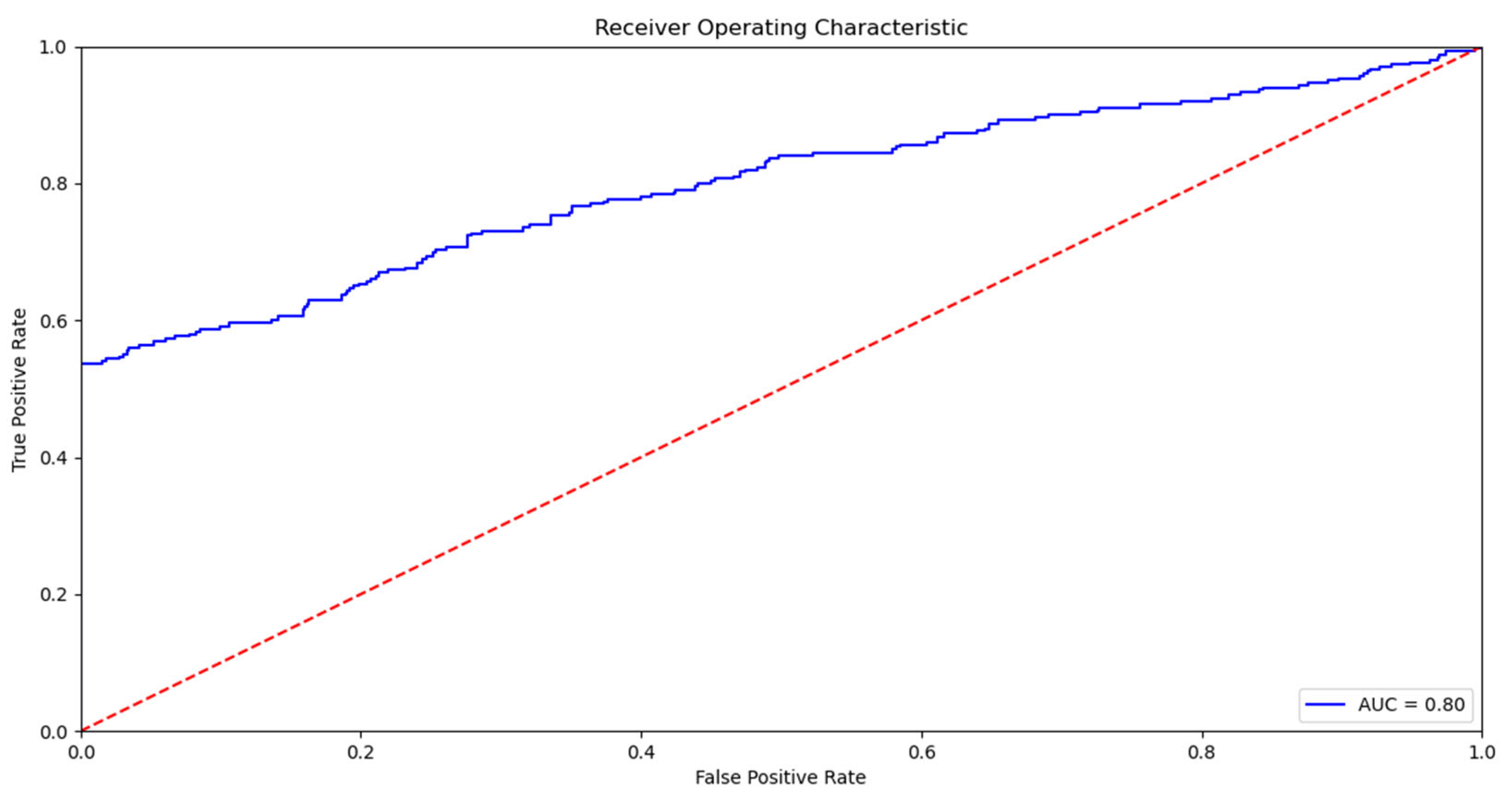
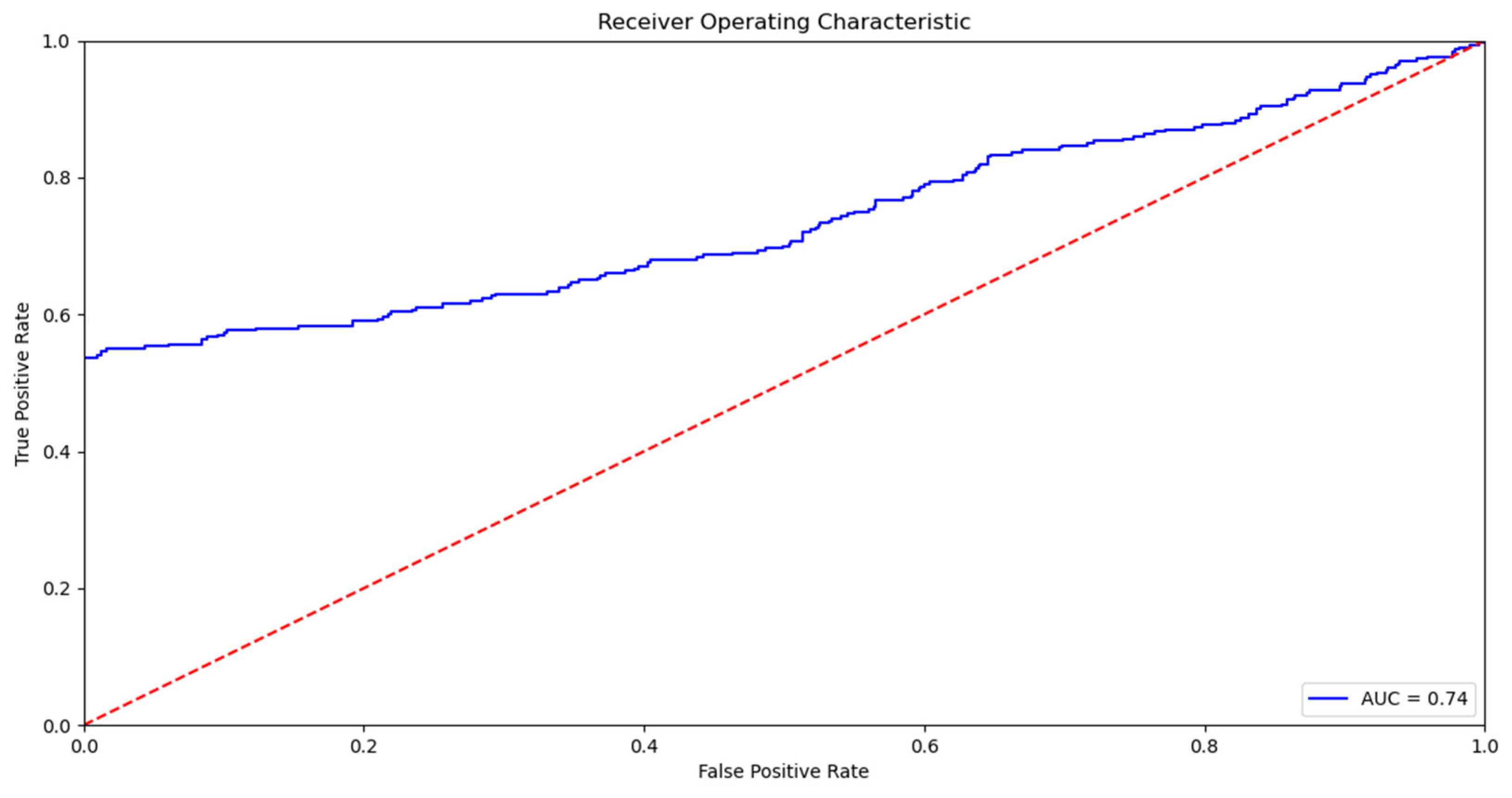
A ROC curve plot was generated to analyze how well the models differentiate between class 1 (mortality) and class 0 (survival). Figure 3 shows the ROC curve of the random forest model that receives the mode matrix every three years as input. The value of 0.8 means that this model has an 80% probability of distinguishing between positive and negative classes. Considering that the objective was to create a mortality predictor as accurately as possible using CHS, it is clear that the random forest model performs a good prediction with this result. Figure 4 and Figure 5 show the ROC curves of SVM and logistic regression, respectively. With SVM, there is a ROC of 0.76, lower than the RF result but still a good result. Finally, the ROC of logistic regression is 0.74, leading to the conclusion that the logistic regression model has the worst performance.

3.3.3. Performance Results after Cross-Validation

Cross-validation was applied to confirm the results and check for overfitting. For this purpose, the initial dataset was separated into ten subsets, and the performance of each one was analyzed, with average performance finally being obtained.

Table 8. Cross-validation results for each model for the matrix created by calculating the mode per year for each variable. K-fold = 10.

Metrics	Random Forest	SVM	Logistic Regression
Accuracy (mean)	0.81 (Train); 0.80 (Test)	0.80 (Train); 0.80 (Test)	0.79 (Train); 0.79 (Test)
F1 Score (mean)	0.76 (Train); 0.75 (Test)	0.75 (Train); 0.75 (Test)	0.74 (Train); 0.72 (Test)
Recall (mean)	0.72 (Train); 0.71 (Test)	0.72 (Train); 0.71 (Test)	0.70 (Train); 0.69 (Test)

shows these results for the mode matrix for all years, while

Table 9. Cross-validation results for each model for the matrix created by calculating mode every 3 years for each variable. K-fold = 10.

Metrics	Random Forest	SVM	Logistic Regression
Accuracy (mean)	0.87 (Train); 0.86 (Test)	0.87 (Train); 0.86 (Test)	0.85 (Train); 0.85 (Test)
F1 Score (mean)	0.80 (Train); 0.80 (Test)	0.80 (Train); 0.79 (Test)	0.79 (Train); 0.79 (Test)
Recall (mean)	0.75 (Train); 0.72 (Test)	0.74 (Train); 0.70 (Test)	0.67 (Train); 0.66 (Test)

shows the results for the mode matrix for every three years.

Table 8 shows the cross-validation results, which indicate that there was no overfitting in the accuracy, F1 score, or recall results. In addition, it confirms that the random forest model has the best performance. On the other hand, the use of the mode matrix every three years (results in Table 9) leads to a better performance than the models trained using the mode matrix for all years (results in Table 8). These results corroborate the idea that adding a temporal change factor to the variables can improve the predictive ability of the algorithms.

3.3.4. Performance Results after PCA

Ninety principal components were applied, which explained 95% of the data variance. In addition, with this process, it was possible to eliminate redundant variables. This behavior was observed in certain cardiovascular variables, such as myocardial infarction, angina, stroke, and heart rate. These variables were expressed in more than one variable, so with PCA, the most helpful variable for the models’ predictions was kept, thanks to which the models slightly improved their performance.

Table 10. Performance for the models after PCA. Values correspond to the model created with the mode matrix by year for each variable.

Metrics	Random Forest	SVM	Logistic Regression
Accuracy (mean)	0.83 (Train); 0.82 (Test)	0.82 (Train); 0.81 (Test)	0.80 (Train); 0.80 (Test)
F1 Score (mean)	0.77 (Train); 0.77 (Test)	0.76 (Train); 0.75 (Test)	0.75 (Train); 0.74 (Test)
Recall (mean)	0.75 (Train); 0.74 (Test)	0.74 (Train); 0.73 (Test)	0.73 (Train); 0.72 (Test)

and

Table 11. Performance for the models after PCA. Values correspond to the model created with the mode matrix every 3 years by variable.

Metrics	Random Forest	SVM	Logistic Regression
Accuracy (mean)	0.89 (Train); 0.88 (Test)	0.88 (Train); 0.88 (Test)	0.86 (Train); 0.85 (Test)
F1 Score (mean)	0.85 (Train); 0.85 (Test)	0.83 (Train); 0.82 (Test)	0.80 (Train); 0.80 (Test)
Recall (mean)	0.80 (Train); 0.80 (Test)	0.78 (Train); 0.77 (Test)	0.77 (Train); 0.77 (Test)

show the performance of the models after PCA for the two feature matrices.

As can be seen in the results shown in Table 10 and Table 11, the application of principal components, in addition to slightly reducing the number of variables, also improved the performance of the three models to some extent. For example, the accuracy of the random forest results in Table 11 is much closer to 90%, and the F1 value and recall also increased to 85% and 80%, respectively.

3.3.5. Confusion Matrices for the Models with the Two Feature Matrices

The confusion matrix was calculated for each of the models implemented in order to see the rates of true positives, true negatives, false positives, and false negatives. Figure 6 shows the values corresponding to the models trained with the mode matrix for all years. Figure 7 shows the results of the models trained with the second mode matrix every 3 years.

The number of true positives and true negatives shows that the random forest has the best performance, since it has the highest values in these two cases, with this behavior being evident in both feature matrices. At the same time, the random forest has the lowest false positives and false negatives in the two matrices. However, the results of the mode matrix every three years are slightly better than those of the first matrix in all three models. In conclusion, it is clear that creating a matrix that maintains a temporal change in the data allows the models to predict a higher number of true positives and true negatives while keeping the number of false positives and false negatives to a minimum.

Table 12. Most important features in random forest mortality prediction.

Feature	Gini Importance
Myocardial infarction	0.75
Angina	0.75
Age	0.73
Bypass surgery	0.69
Health category (how healthy is the patient?)	0.63
Cardiovascular health failure	0.63
Coronary heart disease Major electrocardiogram abnormalities	0.61
Diabetes	0.56
Other heart and circulation problems	0.52
Weakness level	0.48

shows the variables that have the greatest influence on the prediction of the random forest model using Gini importance or mean decrease in impurity. Gini importance “indicates how often a particular feature θ was selected for a split, and how large its overall discriminative value was for the classification problem under study” [35].

4. Discussion and Conclusions

4.1. Discussion

The calculation of the accuracy, F1 value, and recall demonstrates that the random forest model has the highest performance. In addition, it is shown that the use of the matrix created from the calculation of the mode every three years improves the performance of the models. In the application of cross-validation, the models presented an excellent performance in each of the divisions of the K-fold cross-validation, so it can be concluded that the models are not overfitted. Although it is not possible to directly compare the model in this study to similar models found in the literature, it can be stated that this model produces similar or improved results.

After applying principal components, it was shown that with 90 variables, 95% of the variance of the data is explained; in addition, when using the classification models, it can be observed that the results improve slightly. In terms of accuracy, the random forest model approaches 90% thanks to the application of PCA. The ROC curves verify the initial result showing that the random forest model can better differentiate the two classes (1 and 0) with an area under the curve (AUC) of 0.80, followed by SVM with an AUC of 0.76 and logistic regression with an AUC of 0.74. With regard to the results from the confusion matrices, it was verified once again that the random forest model is the one with the best performance since it has a higher number of TPs and TNs and a lower number of FPs and FNs than the other two models. In addition, the use of the matrix every three years improves the results of the three models, so the use of a matrix that maintains a temporal change in the variables allows the models to make more accurate predictions.

The aim of this study was to predict mortality based on cardiovascular variables, medical history (including some multiple chronic conditions), medications, and electrocardiogram variables. According to the resulting random forest model, the most relevant variables to predict mortality were myocardial infarction, hypertension, angina, heart failure, arthritis, chronic respiratory conditions, diabetes, and cancer-related variables. Although the variables angina and myocardial infarction have high Gini importance, if only these two variables are used, the model is not able to obtain a similar result under the same conditions. Thus, the model needs to be fed to other closely related variables, such as age, other variables related to MCC, and cardiovascular variables, to obtain an accurate result. When applying principal component analysis, it was seen that the number of variables did not decrease significantly. Consequently, it is demonstrated that all of the variables have importance when predicting mortality in older adult patients.

The dataset used in this study may be outdated, as the last year of measurements used was 2000. This is a limitation, so this study should be updated to consider medical advances. However, the variables found in CHS made it possible to perform analyses and create models that confirm the relationship between mortality risk and the variables mentioned in this study. It should be mentioned that CHS is one of the few open databases for secondary analysis in the field. Finally, the experiments did not consider variables related to daily life activities to build the model in this study, which only uses the variable level of depression available in the database. Thus, more variables should be included in future studies.

4.2. Conclusions

In the first place, the literature reviewed revealed that readmissions, hospitalizations, and mortality are frequent in patients with cardiovascular pathologies, especially those with CHD. In addition, it was established that some of the main variables influencing patients’ hospitalization, readmission, and mortality are hypertension, systolic pressure, diastolic pressure, heart rate, gender, age, and body mass index. Finally, studies usually analyze cardiovascular disease risk factors and predict pathologies such as cerebrovascular infarction and coronary artery disease. No studies have been observed that associate clinical mortality outcomes with multiple chronic conditions and cardiovascular diseases. This study proposes supervised models to predict patients’ mortality risk from cardiovascular variables, medical history, medications, and electrocardiogram variables, including a summary of data that takes into consideration some temporal variation. The accuracy of random forest models was between 0.83 and 0.89, which are similar or, in some cases, better results than those in the literature. These are mostly survival models based on Cox regression or supervised learning with methodologies other than the one implemented. The final conclusion is that the models respond to the objective of predicting mortality risk in older adult patients with cardiovascular pathologies and multiple chronic diseases (MCC).

This research employed a series of algorithms based on supervised learning that can accurately predict patient mortality using the CHS database. Future work will seek to improve the performance of the models with other preprocessing methods and machine learning models. In addition, the algorithm will be extended to predict other events, such as hospitalization. In addition, different approaches based on deep learning algorithms will be tested to perform the prediction, such as LSTM or artificial neural networks. Finally, more specific studies will be conducted to determine the effect of MCCs in different combinations in predicting mortality, and the models will be tested on other databases so that the models can be adapted to different cases.

Thus, this study resulted in an algorithm to predict mortality. However, in the future, this algorithm could benefit health professionals in a practical way if the model were implemented through a web or desktop application into which they could enter patient data and receive a prediction.

References

1. About Chronic Diseases. National Center for Chronic Disease Prevention and Health Promotion. Available online: https://www.cdc.gov/chronicdisease/about/index.htm (accessed on 24 June 2022).
2. Chronic Conditions Chartbook. Centers for Medicare and Medicaid Services. Available online: https://www.cms.gov/Research-Statistics-Data-and-Systems/Statistics-Trends-and-Reports/Chronic-Conditions/2012ChartBook (accessed on 24 June 2022).
3. HHS Initiative on Multiple Chronic Conditions 2014. U.S. Department of Health and Human Services. Available online: http://www.hhs.gov/ash/initiatives/mcc/ (accessed on 1 October 2022).
4. Javaid, M.; Haleem, A.; Pratap Singh, R.; Suman, R.; Rab, S. Significance of machine learning in healthcare: Features, pillars and applications. Int. J. Intell. Netw. 2022, 3, 58–73. [Google Scholar] [CrossRef]
5. Liu, S.; Du, H.; Feng, M. Robust Predictive Models in Clinical Data—Random Forest and Support Vector Machines. In Leveraging Data Science for Global Health; Celi, L.A., Majumder, M.S., Ordóñez, P., Osorio, J.S., Paik, K.E., Somai, M., Eds.; Springer International Publishing: New York, NY, USA, 2020; pp. 219–228. [Google Scholar]
6. Rodgers, J.L.; Jones, J.; Bolleddu, S.I.; Vanthenapalli, S.; Rodgers, L.E.; Shah, K.; Karia, K.; Panguluri, S.K. Cardiovascular Risks Associated with Gender and Aging. J. Cardiovasc. Dev. Dis. 2019, 6, 19. [Google Scholar] [CrossRef] [PubMed] [Green Version]
7. Yang, J.; Ju, X.; Liu, F.; Asan, O.; Church, T.; Smith, J. Prediction for the Risk of Multiple Chronic Conditions Among Working Population in the United States With Machine Learning Models. IEEE Open J. Eng. Med. Biol. 2021, 2, 291–298. [Google Scholar] [CrossRef] [PubMed]
8. Kawano, K.; Otaki, Y.; Suzuki, N.; Fujimoto, S.; Iseki, K.; Moriyama, T.; Yamagata, K.; Tsuruya, K.; Narita, I.; Kondo, M.; et al. Prediction of mortality risk of health checkup participants using machine learning-based models: The J-SHC study. Sci. Rep. 2022, 12, 14154. [Google Scholar] [CrossRef] [PubMed]
9. Di Castelnuovo, A.; Bonaccio, M.; Costanzo, S.; Gialluisi, A.; Antinori, A.; Berselli, N.; Blandi, L.; Bruno, R.; Cauda, R.; Guaraldi, G.; et al. Common cardiovascular risk factors and in-hospital mortality in 3894 patients with COVID-19: Survival analysis and machine learning-based findings from the multicentre Italian CORIST Study. Nutr. Metab. Cardiovasc. Dis. 2020, 30, 1899–1913. [Google Scholar] [CrossRef] [PubMed]
10. Mirkin, K.A.; Enomoto, L.M.; Caputo, G.M.; Hollenbeak, C.S. Risk factors for 30-day readmission in patients with congestive heart failure. Heart Lung 2017, 46, 357–362. [Google Scholar] [CrossRef] [PubMed]
11. Kaiser, P.; Allen, N.; Delaney, J.A.C.; Hirsch, C.H.; Carnethon, M.; Arnold, A.M.; Odden, M.C. The association of prediagnosis social support with survival after heart failure in the Cardiovascular Health Study. Ann. Epidemiol. 2020, 42, 73–77. [Google Scholar] [CrossRef] [PubMed]
12. Ali, N.H.; Abozead, S.E.-S.; Ahmed, A.A.G.; Abd El-All, H.A.E. Risk Factors for Frequency of Readmission among Heart Failure Patients. Assiut Sci. Nurs. J. 2020, 8, 147–153. [Google Scholar] [CrossRef]
13. Daghistani, T.A.; Elshawi, R.; Sakr, S.; Ahmed, A.M.; Al-Thwayee, A.; Al-Mallah, M.H. Predictors of in-hospital length of stay among cardiac patients: A machine learning approach. Int. J. Cardiol 2019, 288, 140–147. [Google Scholar] [CrossRef] [PubMed]
14. Guo, A.; Pasque, M.; Loh, F.; Mann, D.L.; Payne, P.R.O. Heart Failure Diagnosis, Readmission, and Mortality Prediction Using Machine Learning and Artificial Intelligence Models. Curr. Epidemiol. Rep. 2020, 7, 212–219. [Google Scholar] [CrossRef]
15. Segar, M.W.; Vaduganathan, M.; Patel, K.V.; McGuire, D.K.; Butler, J.; Fonarow, G.C.; Basit, M.; Kannan, V.; Grodin, J.L.; Everett, B.; et al. Machine Learning to Predict the Risk of Incident Heart Failure Hospitalization Among Patients with Diabetes: The WATCH-DM Risk Score. Diabetes Care 2019, 42, 2298–2306. [Google Scholar] [CrossRef] [PubMed]
16. Mezzatesta, S.; Torino, C.; Meo, P.; Fiumara, G.; Vilasi, A. A machine learning-based approach for predicting the outbreak of cardiovascular diseases in patients on dialysis. Comput. Methods Programs Biomed. 2019, 177, 9–15. [Google Scholar] [CrossRef] [PubMed]
17. da Silva, D.B.; Schmidt, D.; da Costa, C.A.; da Rosa Righi, R.; Eskofier, B. DeepSigns: A predictive model based on Deep Learning for the early detection of patient health deterioration. Expert Syst. Appl. 2021, 165, 113905. [Google Scholar] [CrossRef]
18. Kavitha, M.; Gnaneswar, G.; Dinesh, R.; Sai, Y.R.; Suraj, R.S. Heart Disease Prediction using Hybrid machine Learning Model. In Proceedings of the 2021 6th International Conference on Inventive Computation Technologies (ICICT), Coimbatore, India, 20–22 January 2021; pp. 1329–1333. [Google Scholar] [CrossRef]
19. Miao, F.; Cai, Y.P.; Zhang, Y.X.; Li, Y.; Zhang, Y.T. Risk Prediction of One-Year Mortality in Patients with Cardiac Arrhythmias Using Random Survival Forest. Comput. Math Methods Med. 2015, 2015, 303250. [Google Scholar] [CrossRef] [PubMed] [Green Version]
20. Huang, Y.-C.; Li, S.-J.; Chen, M.; Lee, T.-S.; Chien, Y.-N. Machine-Learning Techniques for Feature Selection and Prediction of Mortality in Elderly CABG Patients. Healthcare 2021, 9, 547. [Google Scholar] [CrossRef] [PubMed]
21. Imamovic, D.; Babovic, E.; Bijedic, N. Prediction of mortality in patients with cardiovascular disease using data mining methods. In Proceedings of the 2020 19th International Symposium INFOTEH-JAHORINA (INFOTEH), East Sarajevo, Bosnia and Herzegovina, 18–20 March 2020; pp. 1–4. [Google Scholar] [CrossRef]
22. Fried, L.P.; Borhani, N.O.; Enright, P.; Furberg, C.D.; Gardin, J.M.; Kronmal, R.A.; Kuller, L.H.; Manolio, T.A.; Mittelmark, M.B.; Newman, A.; et al. The Cardiovascular Health Study: Design and rationale. Ann. Epidemiol. 1991, 1, 263–276. [Google Scholar] [CrossRef]
23. Towards Data Science. Missing Data Imputation Concepts and Techniques about How to Handle Missing Data Imputation. Available online: https://towardsdatascience.com/missing-data-imputation-5c664ad77ef (accessed on 24 June 2022).
24. Louca, P.; Tran, T.Q.B.; Toit, C.d.; Christofidou, P.; Spector, T.D.; Mangino, M.; Suhre, K.; Padmanabhan, S.; Menni, C. Machine learning integration of multimodal data identifies key features of blood pressure regulation. Ebiomedicine 2022, 84, 104243. [Google Scholar] [CrossRef] [PubMed]
25. Towards Data Science. All about Feature Scaling Scale Data for Better Performance of Machine Learning Model. Available online: https://towardsdatascience.com/all-about-feature-scaling-bcc0ad75cb35 (accessed on 24 June 2022).
26. Towards Data Science. Decision Trees and Random Forests—Explained. Available online: https://towardsdatascience.com/decision-tree-and-random-forest-explained-8d20ddabc9dd (accessed on 24 June 2022).
27. Géron, A. Ensemble Learning and Random Forests. In Hands-On Machine Learning with Scikit-Learn, Keras and TensorFlow: Concepts, Tools, and Techniques to Build Intelligent Systems, 2nd ed.; Roumeliotis, R., Tache, N., Eds.; O’Reilly: Sebastopol, CA, USA, 2019; pp. 189–198. ISBN 978-149-203-264-9. [Google Scholar]
28. Géron, A. Support Vector Machines. In Hands-On Machine Learning with Scikit-Learn, Keras and TensorFlow: Concepts, Tools, and Techniques to Build Intelligent Systems, 2nd ed.; Roumeliotis, R., Tache, N., Eds.; O’Reilly: Sebastopol, CA, USA, 2019; pp. 153–172. ISBN 978-149-203-264-9. [Google Scholar]
29. Géron, A. Logistic Regression. In Hands-On Machine Learning with Scikit-Learn, Keras and TensorFlow: Concepts, Tools, and Techniques to Build Intelligent Systems, 2nd ed.; Roumeliotis, R., Tache, N., Eds.; O’Reilly: Sebastopol, CA, USA, 2019; pp. 142–144. ISBN 978-149-203-264-9. [Google Scholar]
30. Géron, A. Better Evaluation Using Cross-Validation. In Hands-On Machine Learning with Scikit-Learn, Keras and TensorFlow: Concepts, Tools, and Techniques to Build Intelligent Systems, 2nd ed.; Roumeliotis, R., Tache, N., Eds.; O’Reilly: Sebastopol, CA, USA, 2019; pp. 73–75. ISBN 978-149-203-264-9. [Google Scholar]
31. Mathemathinking. Recall, Precision, Specificity, and Sensitivity. Available online: http://corysimon.github.io/articles/classification-metrics (accessed on 24 June 2022).
32. Géron, A. Precision and Recall. In Hands-On Machine Learning with Scikit-Learn, Keras and TensorFlow: Concepts, Tools, and Techniques to Build Intelligent Systems, 2nd ed.; Roumeliotis, R., Tache, N., Eds.; O’Reilly: Sebastopol, CA, USA, 2019; pp. 92–93. ISBN 978-149-203-264-9. [Google Scholar]
33. Géron, A. The ROC Curve. In Hands-On Machine Learning with Scikit-Learn, Keras and TensorFlow: Concepts, Tools, and Techniques to Build Intelligent Systems, 2nd ed.; Roumeliotis, R., Tache, N., Eds.; O’Reilly: Sebastopol, CA, USA, 2019; pp. 97–99. ISBN 978-149-203-264-9. [Google Scholar]
34. Géron, A. Confusion Matrix. In Hands-on Machine Learning with Scikit-Learn, Keras and TensorFlow: Concepts, Tools, and Techniques to Build Intelligent Systems, 2nd ed.; Roumeliotis, R., Tache, N., Eds.; O’Reilly: Sebastopol, CA, USA, 2019; pp. 90–92. ISBN 978-149-203-264-9. [Google Scholar]
35. Menze, B.H.; Kelm, B.M.; Masuch, R.; Himmelreich, U.; Bachert, P.; Petrich, W.; Hamprecht, F.A. A comparison of random forest and its Gini importance with standard chemometric methods for the feature selection and classification of spectral data. BMC Bioinform. 2009, 10, 213. [Google Scholar] [CrossRef] [PubMed]
Figure 1. Feature matrix created by calculating the mode per year for each variable.
Applsci 12 11536 g001
Figure 2. Feature matrix created by calculating mode every 3 years for each variable.
Applsci 12 11536 g002
Figure 3. ROC curve of random forest model receiving the mode matrix every 3 years as input.
Applsci 12 11536 g003
Figure 4. ROC curve of SVM model that receives the mode matrix every 3 years as input.
Applsci 12 11536 g004
Figure 5. ROC curve of logistic regression model receiving the mode matrix every 3 years as input.
Applsci 12 11536 g005
Figure 6. Confusion matrices for the models that receive the mode matrix of all years as input.
Applsci 12 11536 g006
Figure 7. Confusion matrices for models receiving the mode matrix every 3 years as input.
Applsci 12 11536 g007