Article

Sliding Mode Path following and Control Allocation of a Tilt-Rotor Quadcopter

Department of Mechanical & Automation Engineering, I-Shou University, Kaohsiung 84001, Taiwan
*
Author to whom correspondence should be addressed.
Appl. Sci. 2022, 12(21), 11088; https://doi.org/10.3390/app122111088
Submission received: 27 September 2022 / Revised: 29 October 2022 / Accepted: 30 October 2022 / Published: 1 November 2022

Abstract

:
A tilt-rotor quadcopter (TRQ) equipped with four tilt-rotors is more agile than its under-actuated counterpart and can fly at any path while maintaining the desired attitude. To take advantage of this additional control capability and enhance the quadrotor system’s robustness and capability, we designed two sliding mode controls (SMCs): the typical SMC exploits the properties of the rotational dynamics, and the modified SMC avoids undesired chattering. Our simulation studies show that the proposed SMC scheme can follow the planned flight path and keep the desired attitude in the presence of variable deviations and external perturbations. We demonstrate from the Lyapunov stability theorem that the proposed control scheme can guarantee the asymptotic stability of the TRQ in terms of position and attitude following via control allocation.

1. Introduction

Due to advancements in microprocessors and sensors, quadrotors have recently received much attention, playing an increasingly important role in unmanned aerial vehicles (UAVs). Now, quadrotors can easily hover indoors or outdoors and fly fast with global positioning system (GPS) devices or tiny cameras. Generally, changing the velocities of rotors [1,2] can generate lift and steering torque to control the attitude and position of the quadcopter.
Scholars and engineers have proposed several methods to solve the control problem for a quadrotor. These methods can be divided into: PID control [3,4,5], feedback linearization [6], optimal control [7], back-stepping [8,9], SMC [10,11,12,13], robust control [14], neural control [15,16], and nonlinear control [17]. To handle uncertainty systematically, researchers have extensively applied SMCs to address the robust control problem of quadrotors.
The super-twist control algorithm [18,19,20], a second-order SMC, has been studied to alleviate harmful chattering and maintain the robust capability of first-order SMCs. The studies in [21,22,23] demonstrate the stability and finite-time convergence of the super-twist control algorithm for single-variable systems through a Lyapunov stability analysis. For instance, Xu et al. [11] studied an adaptive terminal sliding mode for a quadrotor attitude control with specified capability and input saturation. In addition, Besnard et al. [12] proposed an observer-based SMC to address model uncertainty and wind perturbation. The recent work in [24,25] introduced the perturbation observer incorporating enhanced SMC for application in quadrotor UAV control.
Recently, several control methods have been proposed to solve the localization or following problem of under-actuated quadrotors, but these methods are still insufficient and have many shortcomings. For example, if the actuator fails or the rotor is damaged, the quadrotor will crash due to a lack of actuator redundancy to restore attitude and position. Tilt-rotor quadrotors [26] can increase the degree of control freedom and provide control redundancy. Compared with under-actuated quadrotors, full-drive quadrotors have more flexibility than under-actuated quadrotors and have recently attracted the research community’s attention. Ryll et al. [27] proposed a modeling approach for an overdrive quadrotor UAV. They provide a dynamic linearization control that uses higher-order derivatives of the measured output. Hua et al. [28] studied the control of vertical take-off and landing (VTOL) vehicles with bank thrust angle limitation. The proposed control can achieve the primary and secondary goals of asymptotically stabilizing position and direction. Recently, Rashad et al. [29] reviewed various UAV designs with fully actuated multi-rotors, in the literature. They introduced the control allocation matrix to categorize the proposed hardware framework and discussed the criteria for optimizing the UAV design. Zheng et al. [30] introduced the hardware design of an experimental tilt-rotor drone that uses linear servo motors to control the tilt mechanism. The authors also implemented and tested their PD-based translation and attitude control scheme on the fully actuated prototype quadrotor. To control the hovering and fixed-wing flight of a tilt-rotor UAV and the transition between them, Willis et al. [31] proposed a control scheme, which includes a low-level angular rate controller and a variable mixer, and an LQR following control
We propose a TRQ model based on translational and rotational dynamics, perturbation, and model uncertainty. Note that the SMC presented for an under-actuated quadrotor cannot be directly applied to a tilt-rotor quadrotor. We propose an SMC scheme with control allocation, exploiting the structural features of rotational dynamics and avoiding chattering in translational dynamics to further enhance the robustness and capability of TRQ systems.
The paper is organized as follows: Section 2 discusses the TRQ’s dynamics and various drive modes. Section 3 presents the proposed SMC scheme and control assignment. Section 4 provides a stability analysis. In Section 5, the proposed SMC scheme is applied to a TRQ for numerical simulation. Section 6 gives some conclusions.

2. Dynamic Model of a Tilt-Rotor Quadcopter (TRQ) with Various Actuation Modes

This section will establish a dynamic model from the Newton–Euler equation. First, we present the dynamics of the TRQ (Figure 1). Using the variables defined in the nomenclature, we propose various actuation modes from over-actuated, to fully actuated, to under-actuated modes.

2.1. Rotational and Translational Dynamics

The rotation matrix R P i B from the ith rotor frame to the body frame is
R P i B = R Z ( β i ) R X ( α i )
R X ( α i ) = [ 1 0 0 0 cos α i sin α i 0 sin α i cos α i ] ,
and
R Z ( β i ) = [ cos β i sin β i 0 sin β i cos β i 0 0 0 1 ] ,   β i = ( i 1 ) π 2 ,   i = 1 ,   2 ,   3 ,   4 .
The angular velocity is
w P i = R B P i w B + [ α ˙ i 0 w i ] T
We define
  s g n ( x ) = {       1       i f     x   > 0 1       i f     x   < 0
where
w 1 < 0 ,   w 3 < 0   ,   w 2 > 0 ,   w 4 > 0
The rotational dynamics of the TRQ can be formulated as:
τ B = I B w ˙ B + w B × I B w B + i = 1 4 R P i B τ P i
where
  τ P i = I P i w ˙ P i + w P i × I P i w P i τ d i
τ d i = [ 0 0 k m w i 2 s g n ( w i ) ] T
The force in the rotor frame is
T p i = [ 0 0 k f w i 2 ] T
and the toque in body frame is
τ B = i = 1 4 ( O P i B × R P i B T P i )
The transform between body angular rates to the Euler rates is
r ˙ = R T w B
where
R T = [ 1 s ϕ tan θ c ϕ tan θ 0 c ϕ s ϕ 0 s ϕ sec θ c ϕ sec θ ]
and r = [ ϕ θ ψ ] T R 3 is the attitude vector of the roll, the pitch, and the yaw angle. We denote s q i = sin q i and c q i = cos   q i .
Taking the derivative of (8) and ignoring I P i in (4), we have
r ¨ = R ˙ T R T 1 r ˙ + R T I B 1 ( τ B w B × I B w B + i = 1 4 R P i B τ d i )
We denote
τ = i = 1 4 ( O P i B × R P i B T P i ) + i = 1 4 R P i B τ d i
Define the transform matrix
Ψ = R T 1
From (8), we have
w B = Ψ r ˙
It follows from (10) and (12) that
Ψ T I B Ψ r ¨ = Ψ T I B Ψ ˙ r ˙ Ψ T w B × I B w B + Ψ T   τ = [ Ψ T I B Ψ ˙ + Ψ T ( Ψ r ˙ × I B Ψ ) ] r ˙ + Ψ T τ
Considering the perturbation torque τ d , we obtain
H ( r ) r ¨ + C ( r , r ˙ ) r ˙ = Ψ T ( τ + τ d )
where
H ( r ) = Ψ T I B Ψ
C ( r , r ˙ ) = [ Ψ T I B Ψ ˙ + Ψ T ( Ψ r ˙ × I B Ψ ) ]
    Ψ ( r ) = [ 1 0 s θ 0 c ϕ c θ s ϕ 0 s ϕ c θ c ϕ ]
and H ( r )     R 3 × 3 is the inertia matrix, C ( r , r ˙ ) r ˙ R 3 represents the centrifugal and Coriolis forces. τ = [ τ ϕ τ θ τ ψ ] T R 3   is the vector of torques and τ d R 3 is the perturbation torque.
The velocity in F w   is
p ˙ = R B W V B
The derivative of velocity in F B   can be expressed as
V ˙ B = w B × V B + R B T W [ 0 0 g ] T + f m
where
R B W = [ c θ c ψ s ϕ s θ c ψ c ϕ s ψ c ϕ s θ c ψ + s ϕ s ψ c θ s ψ s ϕ s θ s ψ + c ϕ c ψ c ϕ s θ s ψ s ϕ c ψ s θ s ϕ c θ c ϕ c θ ]
and
f = i = 1 4 R P i B T P i
where   p = [ x y z ] T R 3 . f = [ f x f y f z ] T R 3 is the vector of forces.
Taking the derivative of (19), ignoring   R ˙ B W and using (20), the translational dynamics becomes
m p ¨ = R B W = ( w B × V B + f ) [ 0 0 m g ] T + u d
where u d R 3 is the perturbation force in F w .

2.2. Over-Actuated, Fully Actuated, and Under-Actuated Modes

Denote α = [ α 1       α 2       α 3       α 4 ] T , w = [ w 1       w 2       w 3       w 4 ] T , s i = sin α i , and c i = cos α i , one can arrange (21) and (11) as
[ f τ ] = [ K 1 ( α ) K 2 ( α ) ] U ( w )
where
U = [ w 1 2 w 2 2 w 3 2 w 4 2 ] T     K 1 ( α ) = [ 0 k f s 2             0       k f s 4 k f s 1 0 k f s 3           0         k f c 1 k f c 2         k f c 3       k f c 4 ]
K 2 ( α ) = [ 0 L k f c 2 k m s 2 0 L k f c 4 + k m s 4 L k f s 1 k m s 1 0 L k f c 3 + k m s 3 0 L k f s 1 + k m c 1 L k f s 2 k m c 2 L k f s 3 + k m s 3 L k f s 4 k m s 4 ]
Remark 1.
Over-actuated and fully actuated modes.
For over-actuated mode, the vector of tilt angles is
α = [ α 1             α 2             α 3             α 4 ] T
By setting   α 3 =   α 1 ,   α 4 =   α 2   , the vector of tilt angles for fully actuated mode is
α = [ α 1             α 2             α 1             α 2 ] T
Remark 1.
Under-actuated mode.
By setting α = [ 0 0 0 0 ] T , the force and the torque in (23) for the under-actuated mode can be reduced as
[ f z τ ϕ τ θ τ ψ ] = [ k f k f k f k f 0 L k f 0 L k f L k f 0 L k f 0 k m k m k m k m ] U ( w )

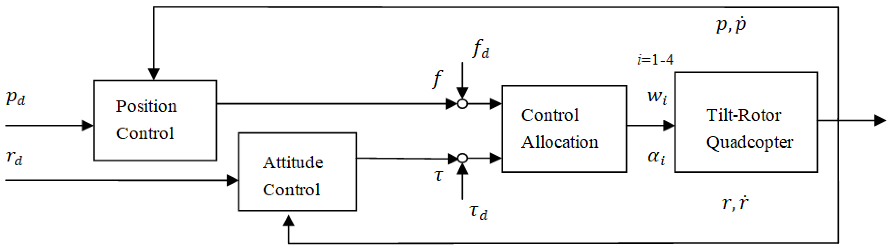
3. Sliding Mode Path following and Control Allocation

In this section, we first propose the sliding mode-based attitude and position following control via torque and force in (23). Then, we present the control allocation from the control torque and force to the speed and tilt angle of four rotors. Figure 2 illustrates the TRQ control scheme.

3.1. Attitude and Position following SMC

Define s 1 R 3
r ˙ r = r ˙ d Λ 1 ( r r d )
and
  s 1 = r ˙ r ˙ r = r ˙ r ˙ d + Λ 1 ( r r d )
where r d is the desired attitude and r ˙ d is the desired angular velocity.
Now, we propose the following control for attitude following to exploit the structure of the rotational dynamics:
  τ = Ψ T [ H ^ r ¨ r + C ^ r ˙ r K 1   S G N ( s 1 ) K 3 s 1 K 4 r ˜ ]
where   r ˜ = r r d and ( · ) ^ denotes the nominal of ( · ) . K 1 ,   K 3 ,   K 4 are positive diagonal matrices, s g n ( · ) is the sign function, and
S G N ( [ x 1     x 2     x 3 ] T ) = [ s g n ( x 1 )     s g n ( x 2 )     s g n ( x 3 ) ] T
We can now define s 2 R 3
  s 2 = p ˙ p ˙ d + Λ 2 ( p p d )
where p d is the desired position and p ˙ d is the desired velocity.
The position following control is proposed to alleviate the chattering effects as follows:
  f = R B 1 W ( u + [ 0 0 m g ]   )  
where u is designed as follows:
u ˙ = ( K 2 + Λ 2 ) u + m ^ ( ( K 2 + Λ 2 ) p ¨ d + p d K 2 Λ 2 ( p ˙ p ˙ d ) Λ 3 s 2 Λ 4   S G N ( s 2 ) )
where   K 2 ,   Λ 2 ,   Λ 3 ,   Λ 4 are positive diagonal matrices.

3.2. Control Allocation

3.2.1. Fully Actuated Mode

We use the following assumption for the fully actuated quadcopter system
    α 3 = α 1 ,       α 4 = α 2
Now, we propose the following steps to compute   α i and w i :
Step 1: Initially, set the tilt angles (   α 1 = α 2 = 0 ) .
Step 2: Compute f and τ from (32) and (29).
Step 3: Compute the rotor velocities.
[ w 1 2 w 2 2 w 3 2 w 4 2 ] = [ k f c 1 k f c 2 k f c 3 k f c 4 0 L k f c 2 k m s 2 0 L k f c 4 + k m s 4 L k f c 1 k m s 1 0 L k f c 3 + k m s 3 0 L k f s 1 + k m c 1 L k f s 2 k m c 2 L k f s 3 + k m c 3 L k f s 4 k m c 4 ] 1 [ f z τ ϕ τ θ τ Ψ ]
where s i = sin α i and c i = cos α i   ( i = 1 ,   2 ,   3 ,   4 ) .
Step 4: Compute the tilt angles from (23) and (24) using (34) as follows:
  α 1 = sin 1 ( f y k f ( w 1 2 + w 3 2 ) ) = α 3
  α 2 = sin 1 ( f x k f ( w 2 2 + w 4 2 ) ) = α 4
Step 5: Go to Step 2 to continue the iteration.

3.2.2. Over-Actuated Mode

We propose the steps to compute   α i and w i :
Step 1: Initially, set the tilt angles   α i = 0   (   i = 1 , 2 , 3 , 4 ) .
Step 2: Compute f and τ from (32) and (29).
Step 3: Compute the rotor velocities from (35).
Step 4: Compute the tilt angles from (23)–(25) as follows:
( k f s 2 ) w 2 2 + ( k f s 4 ) w 4 2 = τ ϕ
( L k f c 2 k m s 2 ) w 2 2 + ( L k f c 4 + k m s 4 ) w 4 2 = τ ϕ
( k f s 1 ) w 1 2 + ( k f s 3 ) w 3 2 = τ θ  
( L k f c 1 k m s 1 ) w 1 2 + ( L k f c 3 + k m s 3 ) w 3 2 = τ θ
where s i = sin α i and c i = cos α i ( i = 1 ,   2 ,   3 ,   4 ) . Using the triangular identities   s i 2 + c i 2 = 1   ( i = 1 ,   2 ,   3 ,   4 ) , one can use the numerical method to solve for α i   in the system of nonlinear equations.
Step 5: Go to Step 2 to continue the iteration.

3.2.3. Under-Actuated Mode

Notice that, due to the lack of control degrees of freedom, the desired attitude ϕ d and θ d is not arbitrary for the under-actuated quadrotor.
One can obtain ϕ d and θ d by
ϕ d = sin 1 ( u x s ψ d u y c ψ d u x   2 + u y   2 + ( u z + m g ) 2 )          
θ d = tan 1 ( u x c ψ d + u y s ψ d u z + m g )                                                  
The vector of w i 2 is
[ w 1 2 w 2 2 w 3 2 w 4 2 ] = [ k f k f k f k f 0 L k f 0 L k f L k f 0 L k f 0 k m k m k m k m ] 1 [ f τ ϕ τ θ τ ψ ]

4. Stability Analysis

This section presents the stability analysis of the SMC scheme. Let us use λ M ( A ) ,   λ m ( A ) for the largest and smallest eigenvalue of a matrix   A . We denote the Euclidean norm for an n × 1 vector x by x = x T x . The inertia matrix is symmetric, positive definite, and bounded by   0 < λ m ( H ) H ( r ) λ M ( H ) . The matrix H ˙ ( r ) 2 C ( r , r ˙ ) is skew-symmetric.

4.1. Sliding Mode Attitude following Control

Theorem 1.
Consider the dynamic model described in (15) and the control for attitude following in (29). The attitude following error dynamics is exponentially stable if the switching gain satisfies the following condition.
  λ m ( K 1 ) ( H ˜ r ¨ r + C ˜ r ˙ r + τ d ) + ε 1
where ε 1 is a positive constant.
Proof. 
H ^ and C ^ represent the nominal H and C , where H ˜ = H H ^ and   C ˜ = C C ^ .
The rotational dynamics can be expressed as follows:
H ^ ( q ) r ¨ + C ^ ( r , r ˙ ) q ˙ = Ψ T ( τ + τ d ) + h 1 ( r , r ˙ , r ¨ )
                    h 1 ( r , r ˙ , r ¨ ) = H ˜ ( r ) r ¨ C ˜ ( r , r ˙ ) r ˙
Define
r ˙ r = r ˙ d Λ 1 ( r r d )
and
s 1 = r ˙ r ˙ r = r ˙ r ˙ d + Λ 1 ( r r d )
It follows from (48) that
s ˙ 1 = r ¨ r ¨ r = r ¨ r ¨ d + Λ 1 ( r ˙ r ˙ d )  
Now, we propose the control
  τ = Ψ T [ H ^ r ¨ r + C ^ r ˙ r K 1   S G N ( s 1 ) K 3 s 1 K 4 r ˜ ]
where   r ˜ = r r d and K 1 ,   K 3 ,   and K 4 are diagonal matrices. □
Define the Lyapunov function
V 1 = 1 2 s 1 T M ( r ) s 1 + 1 2 r ˜ T K 4 r ˜
Using (50) and taking derivative of V 1 yield
V ˙ 1 = s 1 T H s ˙ 1 + 1 2 s 1 T H ˙ s 1 + r ˜ T K 4 r ˜ ˙
If the switching gain meets the condition as follows
  λ m ( K 1 ) ( H ˜ r ¨ r + C ˜ r ˙ r + τ d ) + ε 1
where ε 1 is a positive constant.
From (52), we have
  V ˙ 1 ε 1   s 1 T S G N ( s 1 ) s 1 T K 3 s 1 r ˜ T K 4 r ˜ < 0   ,   s 1 0  
The following adaptation law can replace the switching gain K 1
K 1 = d i a g ( [ k 1     k 2     k 3 ] )    
  k i ( t ) = k c i | η i | + k m i    
where k c i > 0 ,   k m i > 0 and η i   is the obtained by filtering the s g n ( s 1 i ) using a low-pass filter
ζ i   η ˙ i + η i = s g n ( s 1 i ) ,   η i ( 0 ) = 0
where ζ i is a positive constant.

4.2. Sliding Mode Position following Control

Theorem 2.
Consider the translational dynamic model described in (21) and the control for position following in (32)–(33). The position following error dynamics is then asymptotically stable.
Proof. 
The translational dynamics is
  p ¨ = 1 m u + u d m
where
  u = [ u x u y u z ] = R B W f [ 0 0 m g ]
The nominal dynamics is
p ¨ = 1 m ^ u + u ^ d m ^
where m ^ is the nominal mass and u ^ d = 0 .
The sliding surface s 2 R 3 is
s 2 = p ˙ p ˙ d + Λ 2 ( p p d )
Using (57) yields
s ˙ 2 = 1 m ^ u p ¨ d + Λ 2 ( p ˙ p ˙ d )
and
s ˙ 2 = 1 m ^ u ˙ p d + Λ 2 ( s ˙ 2 Λ 2 ( p ˙ p ˙ d )   )
Define the Lyapunov function
V 2 = 1 2 s 2 T Λ 3 s 2 + 1 2 s ˙ 2 T s ˙ 2 + γ A B S ( s 2 )
where
γ = [ γ 1   γ 2   γ 3 ]
It follows from (63) that
V ˙ 2 = s ˙ 2 T ( s ¨ 2 + Λ 3 s 2 + Λ 4   S G N ( s 2 ) )
where Λ 4 is a diagonal matrix with diagonal elements [ γ 1   γ 2   γ 3 ] .
Then
s ¨ 2 + Λ 3 s 2 + Λ 4   S G N ( s 2 ) = K 2 s ˙ 2
and
V ˙ 2 = K 2 s ˙ 2 T s ˙ 2
Using (62) and (65) yields
u ˙ = m ^ ( ( K 2 + Λ 2 ) s ˙ 2 Λ 3 s 2 Λ 4   S G N ( s 2 ) + p d + Λ 2 2 ( p ˙ p ˙ d ) )
Substituting s ˙ 2 from (61) into (64), we have
u ˙ = ( K 2 + Λ 2 ) u + m ^ ( ( K 2 + Λ 2 ) p ¨ d + p d K 2 Λ 2 ( p ˙ p ˙ d ) Λ 3 s 2 Λ 4   S G N ( s 2 ) )
We can derive from LaSalle-Yoshizawa theorem and (66) that s ˙ 2 0 . On the basis of (62) and the Barbalat’s lemma, one can conclude that s ¨ 2 0 . Therefore, we have the following from (65)
Λ 3 s 2 = Λ 4   S G N ( s 2 )  
which ensures that
s 2 = 0

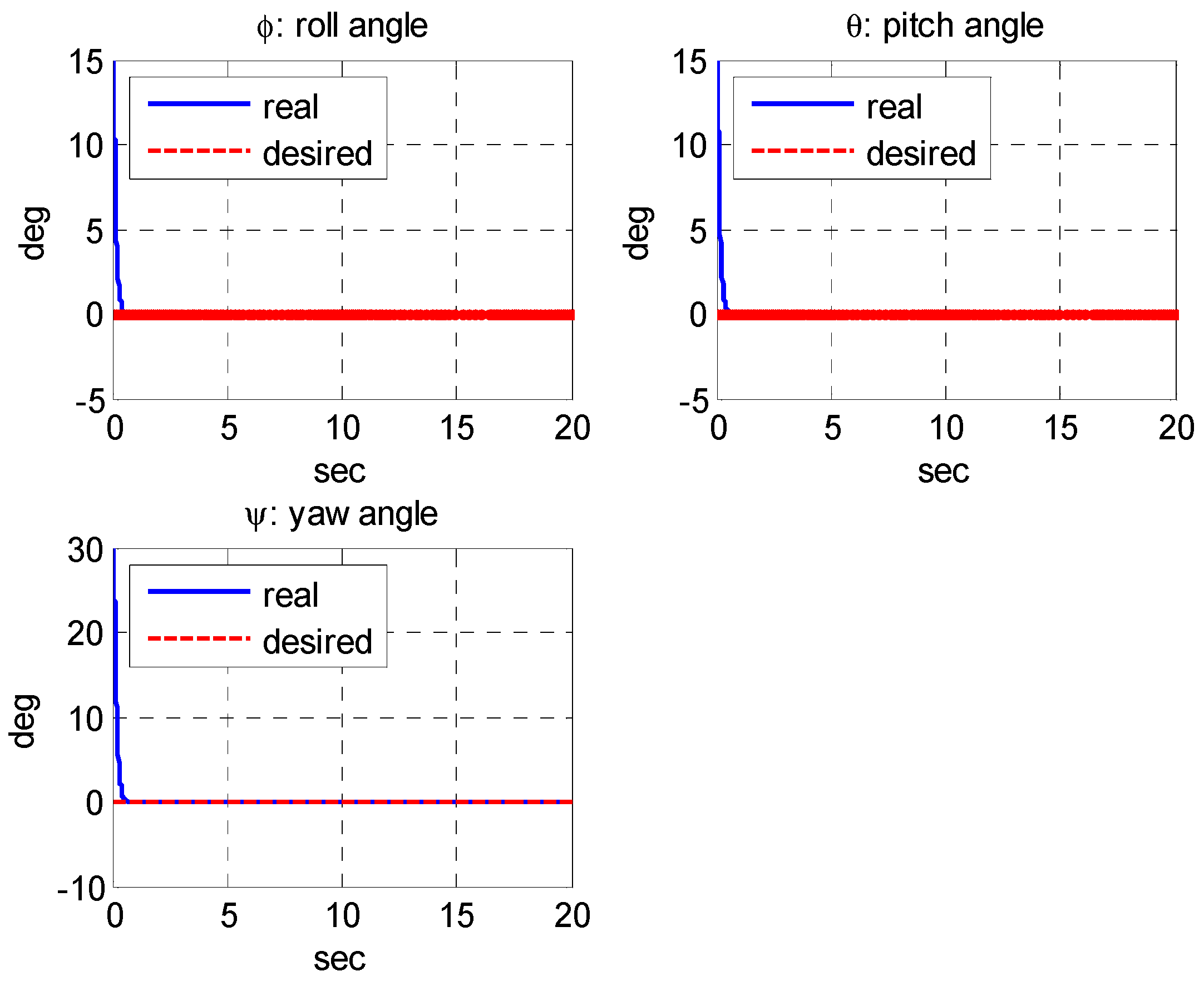
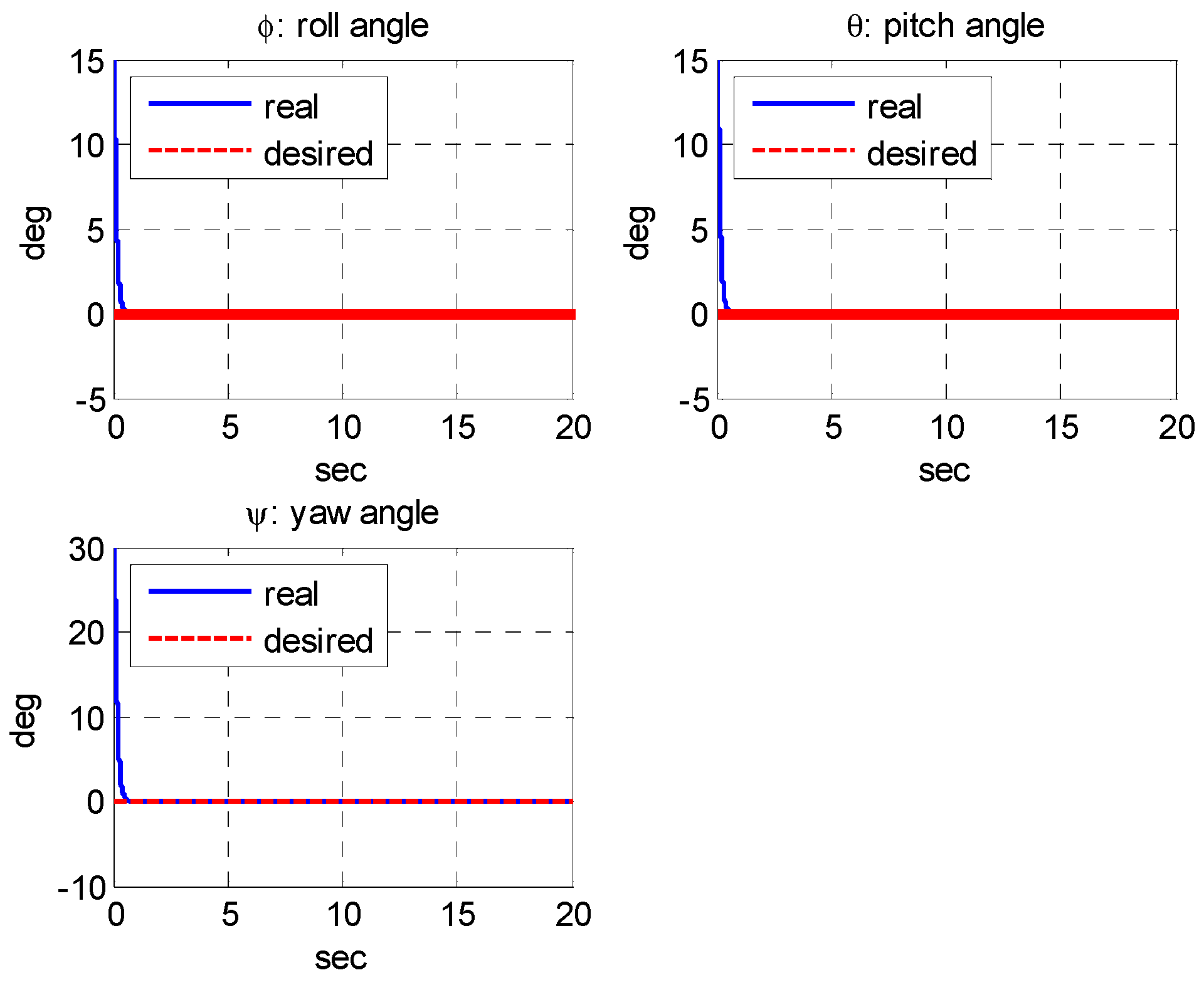
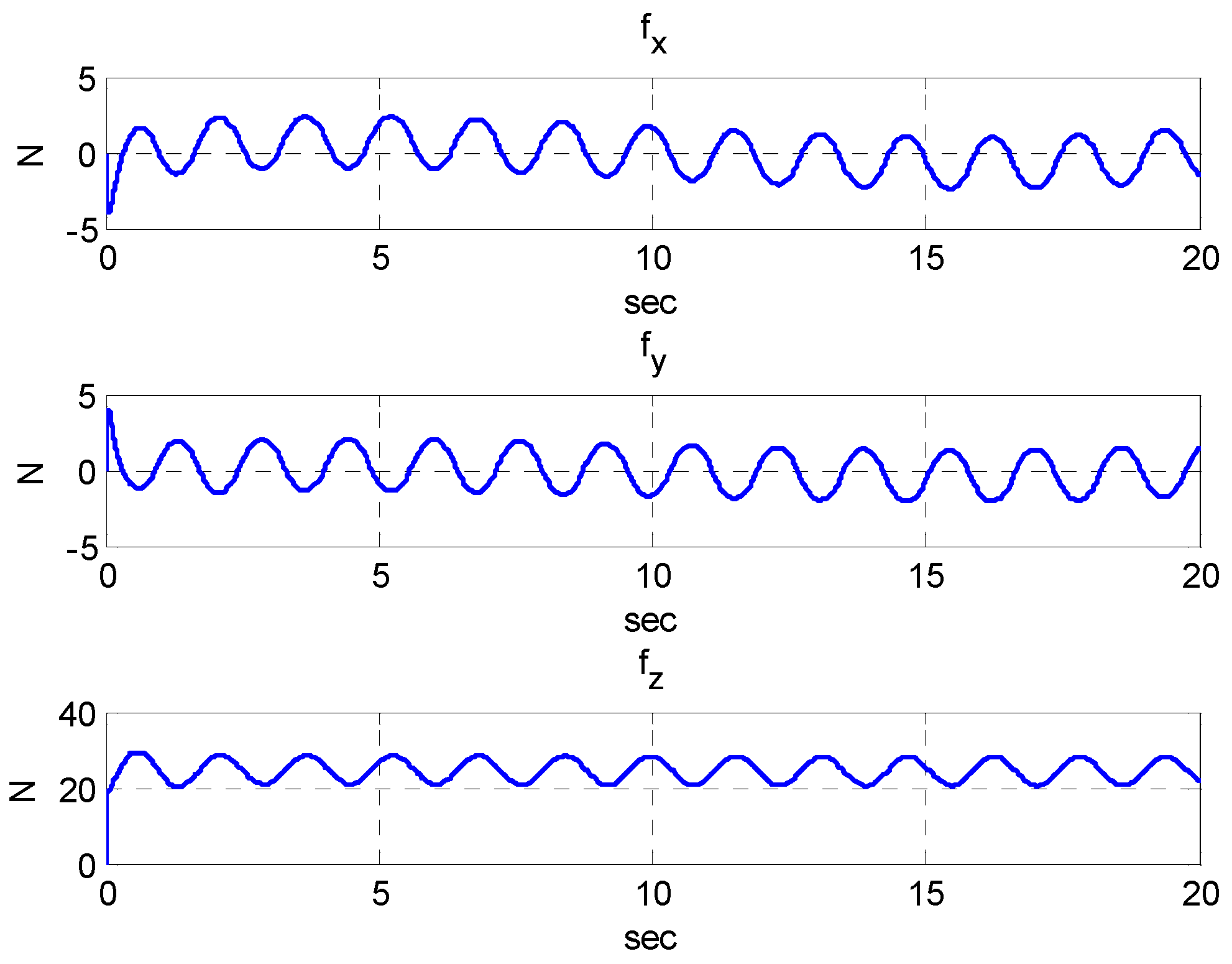
5. Numerical Simulation

To illustrate the proposed control scheme’s design, we give an example of a fully actuated TRQ.

5.1. Simulation Parameters

Assuming s q i = sin q i ,   c q i = cos   q i ,   we have
H 11 = I x , H 12 = 0 ,   H 13 = I x s θ H 22 = I y c ϕ 2 + I z s ϕ 2 ,   H 23 = c θ c ϕ s ϕ ( I y I z ) H 33 = I x s θ 2 + I y c θ 2 s ϕ 2 + I z c θ 2 c ϕ 2
The matrix of C ( r , r ˙ ) is
C 11 = 0 C 12 = I x ψ ˙ c θ + ( I y I z ) ( θ ˙ s ϕ c ϕ + ψ ˙ c θ s ϕ 2 ψ ˙ c θ c ϕ 2 ) C 13 = I y ψ ˙ c θ 2 s ϕ c ϕ + I z ψ ˙ c θ 2 s ϕ c ϕ C 21 = I x ψ ˙ c θ ( I y I z ) ( θ ˙ s ϕ c ϕ + ψ ˙ c θ s ϕ 2 ψ ˙ c θ c ϕ 2 ) C 22 = I y ϕ ˙ s ϕ c ϕ + I z ϕ ˙ s ϕ c ϕ C 23 = I x ψ ˙ s θ c θ + I y ψ ˙ s θ c θ s ϕ 2 + I z ψ ˙ s θ c θ c ϕ 2 C 31 = I x θ ˙ c θ + I y ψ ˙ c θ 2 s ϕ c ϕ I z ψ ˙ c θ 2 s ϕ c ϕ C 32 = I x ψ ˙ s θ c θ + ( I z I y ) ( θ ˙ s θ s ϕ c ϕ + ϕ ˙ c θ s ϕ 2 ϕ ˙ c θ c ϕ 2 ) I y ψ ˙ s θ c θ s ϕ 2 I z ψ ˙ s θ c θ c ϕ 2   C 32 = I x ψ ˙ s θ c θ + ( I z I y ) ( θ ˙ s θ s ϕ c ϕ + ϕ ˙ c θ s ϕ 2 ϕ ˙ c θ c ϕ 2 ) I y ψ ˙ s θ c θ s ϕ 2 I z ψ ˙ s θ c θ c ϕ 2 C 33 = I x θ ˙ s θ c θ + I y ( θ ˙ s θ c θ s ϕ 2 + ϕ ˙ c θ 2 s ϕ c ϕ ) I z ( θ ˙ s θ c θ c ϕ 2 + ϕ ˙ c θ 2 s ϕ c ϕ )
We employ the following variables for simulation:
m = 2 kg ,   L = 0.275 m , g = 9.81 m / s 2 , I x = 0.025 kgm 2 ,   I y = 0.025 kgm 2 , I z = 0.040 kgm 2 , k m = 2.67 · 10 7 Ns 2 ,   k f = 1.5 · 10 5 Nms 2 .
with initial conditions
[ x ( 0 ) y ( 0 ) z ( 0 ) ] = [ 0 0 0 ]
and the desired positions
[ x d ( t f ) y d ( t f ) z d ( t f ) ] = [ 20 10 5 ]
where t f = 20 . The desired attitudes are
ϕ d = 0 ,   θ d = 0 ,   ψ d = 0
The desired path is defined as
x d ( t ) = 2.5 · 10 2   t 3 1.875 · 10 3   t 4 + 3.75 · 10 5   t 5 y d ( t ) = 1.25 · 10 2   t 3 9.375 · 10 4   t 4 + 1.875 · 10 5   t 5 z d ( t ) = 6.25 · 10 3   t 3 4.6875 · 10 4   t 4 + 9.375 · 10 6   t 5
Now, we use the following control parameters for simulation:
Λ 1 = 10   I 2   , Λ 2 = 4 I 3 ,   Λ 3 = 40   I 3 ,   Λ 4 = I 3 , K 1 = I 3 , K 2 = 4 I 3 , K 3 = 4 I 3 ,   K 4 = 10 I 3 , k c i = 4 I 3 ,     k m i = 0.1 I 3 ,     ( i = 1 , 2 , 3 ) .

5.2. Simulation Results

We present the simulation results of the proposed attitude and position following SMC control in Figure 3, Figure 4, Figure 5, Figure 6, Figure 7 and Figure 8. Figure 3 and Figure 4 show the attitude and position trajectories of the quadrotor with variable changes (weights increased to 125%). The simulation results in Figure 3 and Figure 4 show that the proposed SMC can successfully drive the quadrotor from the initial position through the desired path to the final destination while maintaining the desired attitude. Figure 5 and Figure 6 show the lift and steering torque produced by the four tilt-rotors of the TRQ. Figure 7 shows the path of the tilt angle with parameter deviation. The corresponding quadrotor speeds are shown in Figure 8.
Because the stability analysis in the previous section demonstrated robustness with respect to parameter uncertainty and external perturbations, we then further evaluated the impact of external perturbations on the TRQ. We used perturbation force [sin(4t) − sin(4t) 2sin(4t)] N and perturbation torque [0.1sin(2t) 0.1sin(2t) 0.1sin(2t)] Nm applied to TRQ for simulated motion. As shown in Figure 9, Figure 10, Figure 11, Figure 12, Figure 13 and Figure 14, we can see that the perturbation has little effect on the capability of the quadcopter because the proposed control and control assignment can reject the perturbation and return the state variables to the sliding surface.
In summary, the numerical simulation results clearly show that the proposed SMC schemes can accomplish the goal of trajectory tracking and counter the parametric variation and external disturbances in the rotation and translation of TRQ via control allocation.

6. Conclusions

This paper presents the dynamic modeling, path following, and control allocation of a TRQ. Two types of SMC are proposed to enhance the robustness and capability: one is the first-order sliding mode for attitude following and the other is the second-order sliding mode for position following. Considering the parameter changes and external perturbation, we show the stability analysis based on the Lyapunov theory that the proposed control scheme can ensure the error dynamics’ asymptotic stability for the position and attitude following. In the numerical simulation of the fully actuated mode, we demonstrated that the proposed SMC could achieve path following and attitude regulation goals in the presence of variable changes and external perturbations. The tilt-rotor quadrotor has more control degrees of freedom than the under-actuated quadrotor and, therefore, can make full use of the control redundancy to complete the simultaneous trajectory tracking and attitude control that a traditional quadrotor cannot do, and thus has a certain degree of actuator fault tolerance. In the future, we will integrate the sliding mode path following and control allocation into a fault-tolerant flight control.

Author Contributions

Conceptualization, C.-C.Y. and S.-J.W.; methodology, C.-C.Y. and S.-J.W.; software, S.-J.W.; validation, C.-C.Y. and S.-J.W.; formal analysis, C.-C.Y.; investigation, S.-J.W.; writing—original draft preparation, C.-C.Y. and S.-J.W.; writing—review and editing, C.-C.Y.; visualization, S.-J.W. All authors have read and agreed to the published version of the manuscript.

Funding

This research received no external funding.

Institutional Review Board Statement

Not applicable.

Informed Consent Statement

Not applicable.

Data Availability Statement

No new data were created or analyzed in this study. Data sharing is not applicable to this article.

Conflicts of Interest

The authors declare no conflict of interest.

Nomenclature

B quadrotor   body
P i propeller   i
F w inerita   world   frame
F B body   frame
F P i i th   propeller   frame
R T   transform   matrix   from   body   angular   rates   to   Euler   rates
p position   of   B   in   F w  
q   Euler   angle   of   B   in   F w
R B W   rotation   matrix   from   F B   to   F w
R P i B   rotation   matrix   from   F P i to   F B
w i i th   propeller   spinning   velocity   about   Z P i
w P i the   angular   velocity   in   the   ith   propeller   frame  
α i i th   propeller   tilting   angle   about   X P i
T P i the   force   in   the   ith   propeller   frame
w B angular   velocity   of   B   in   F B
v B velocity   of   B   in   F B
τ B torque   in   F B
τ P i torque   in   F P i
τ d i i th   propeller   air   drag   torque   about   Z P i
T i i th   propeller   thrust   along   Z P i
τ w i   motor   torque   along   Z P i
m total   quadrotor   mass
I P i inertia   of   the   ith   propeller   P i
I B inertia   of   the   quadcopter   body   B
k f propeller   thrust   coefficient
k m propeller   drag   coefficient
L distance   of   F P i   to   F B
g gravity   constant

References

  1. Mahony, R.; Kumar, V.; Corke, P. Multirotor Aerial Vehicles: Modeling, Estimation, and Control of Quadrotor. IEEE Robot. Autom. Mag. 2012, 19, 20–32. [Google Scholar] [CrossRef]
  2. Quan, Q. Introduction to Multicopter Design and Control; Springer: Berlin/Heidelberg, Germany, 2017. [Google Scholar]
  3. Miranda-Colorado, R.; Aguilar, L.T. Robust PID control of quadrotors with power reduction analysis. ISA Trans. 2020, 98, 47–62. [Google Scholar] [CrossRef] [PubMed]
  4. Gomes, L.L.; Leal, L.; Oliveira, T.R.; Cunha, J.P.V.S.; Revoredo, T.C. Unmanned Quadcopter Control Using a Motion Capture System. IEEE Lat. Am. Trans. 2016, 14, 3606–3613. [Google Scholar] [CrossRef]
  5. Shankaran, V.P.; Azid, S.I.; Mehta, U.; Fagiolini, A. Improved Performance in Quadrotor Trajectory Tracking Using MIMO PI-D Control. IEEE Access 2022, 10, 110646–110660. [Google Scholar]
  6. Lee, D.; Kim, H.J.; Sastry, S. Feedback Linearization vs. Adaptive SMC for a Quadrotor Helicopter. Int. J. Control Autom. Syst. 2009, 7, 419–428. [Google Scholar] [CrossRef]
  7. Satici, A.C.; Poonawala, H.; Spong, M.W. Robust Optimal Control of Quadrotor UAVs. IEEE Access 2013, 1, 79–93. [Google Scholar] [CrossRef]
  8. Koksal, N.; An, H.; Fidan, B. Backstepping-based adaptive control of a quadrotor UAV with guaranteed following capability. ISA Trans. 2020, 105, 98–110. [Google Scholar] [CrossRef]
  9. Young-Cheol, C.; Hyo-Sung, A. Nonlinear Control of Quadrotor for Point Following: Actual Implementation and Experimental Tests. IEEE/ASME Trans. Mechatron. 2015, 20, 1179–1192. [Google Scholar]
  10. Perozzi, G.; Efimov, D.; Biannic, J.-M.; Planckaert, L. Path following for a quadrotor under wind perturbations: SMC with state-dependent gains. J. Frankl. Inst. 2018, 355, 4809–4838. [Google Scholar] [CrossRef] [Green Version]
  11. Xu, G.; Xia, Y.; Zhai, D.-H.; Ma, D. Adaptive prescribed capability terminal sliding mode attitude control for quadrotor under input saturation. IET Control Theory Appl. 2020, 14, 2473–2480. [Google Scholar] [CrossRef]
  12. Besnard, L.; Shtessel, Y.B.; Landrum, B. Quadrotor vehicle control via SMCler driven by sliding mode perturbation observer. J. Frankl. Inst. 2012, 349, 658–684. [Google Scholar] [CrossRef]
  13. Ricardo, J.A., Jr.; Santos, D.A.; Oliveira, T.R. Attitude Tracking Control for a Quadrotor Aerial Robot Using Adaptive Sliding Modes. In Proceedings of the XLI Ibero-Latin-American Congress on Computational Methods in Engineering (ABMEC), Foz do Iguaçu, Brazil, 16–19 November 2020. [Google Scholar]
  14. Islam, S.; Liu, P.X.; El Saddik, A. Robust Control of Four-Rotor Unmanned Aerial Vehicle With Perturbation Uncertainty. IEEE Trans. Ind. Electron. 2015, 62, 1563–1571. [Google Scholar] [CrossRef]
  15. Dierks, T.; Jagannathan, S. Output Feedback Control of a Quadrotor UAV Using Neural Networks. IEEE Trans. Neural Netw. 2010, 21, 50–66. [Google Scholar] [CrossRef] [PubMed]
  16. Wu, H.; Ye, H.; Xue, W.; Yang, X. Improved Reinforcement Learning Using Stability Augmentation With Application to Quadrotor Attitude Control. IEEE Access 2022, 10, 67590–67604. [Google Scholar] [CrossRef]
  17. Yang, S.; Xian, B. Exponential Regulation Control of a Quadrotor Unmanned Aerial Vehicle With a Suspended Payload. IEEE Trans. Control Syst. Technol. 2020, 28, 2762–2769. [Google Scholar] [CrossRef]
  18. Levant, A. Principles of 2-sliding mode design. Automatica 2007, 43, 576–586. [Google Scholar] [CrossRef] [Green Version]
  19. Levant, A. Sliding order and sliding accuracy in SMC. Int. J. Control 1993, 58, 1247–1263. [Google Scholar] [CrossRef]
  20. Utkin, V.I.; Poznyak, A.S. Adaptive SMC with application to super-twist algorithm: Equivalent control method. Automatica 2013, 49, 39–47. [Google Scholar] [CrossRef]
  21. Moreno, A.; Osorio, M. Strict Lyapunov functions for the super-twisting algorithm. IEEE Trans. Autom. Control 2012, 57, 1035–1040. [Google Scholar] [CrossRef]
  22. Pico, J.; Pico-Marco, E.; Vignoni, A.; De Battista, H. Stability preserving maps for finite-time convergence: Super-twisting sliding-mode algorithm. Automatica 2013, 49, 534–539. [Google Scholar] [CrossRef]
  23. Utkin, V. On convergence time and perturbation rejection of super-twisting control. IEEE Trans. Autom. Control 2013, 58, 2013–2017. [Google Scholar] [CrossRef]
  24. Mokhtari, A.; Benallegue, A.; Orlov, Y. Exact linearization and sliding mode observer for a quadrotor unmanned aerial vehicle. Int. J. Robot. Autom. 2006, 21, 39–49. [Google Scholar] [CrossRef]
  25. Beballegue, A.; Mokhtari, A.; Fridman, L. High-order sliding-mode observer for a quadrotor UAV. Int. J. Robust Nonlinear Control 2008, 18, 427–440. [Google Scholar] [CrossRef]
  26. Bauersfeld, L.; Spannagl, L.; Ducard, G.J.J.; Onder, C.H. MPC Flight Control for a Tilt-Rotor VTOL Aircraft. IEEE Trans. Aerosp. Electron. Syst. 2021, 57, 2395–2409. [Google Scholar] [CrossRef]
  27. Ryll, M.; Bülthoff, H.H.; Giordano, P.R. A Novel Overactuated Quadrotor UnmannedAerial Vehicle: Modeling, Control, and Experimental Validation. IEEE Trans. Control Syst. Technol. 2015, 23, 540–556. [Google Scholar] [CrossRef] [Green Version]
  28. Hua, M.-D.; Hamel, T.; Morin, P.; Samson, C. Control of VTOL vehicles with thrust-tilting augmentation. Automatica 2015, 52, 1–7. [Google Scholar] [CrossRef] [Green Version]
  29. Rashad, R.; Goerres, J.; Aarts, R.; Engelen, J.B.C.; Stramigioli, S. Fully Actuated Multirotor UAVs: A Literature Review. IEEE Robot. Autom. Mag. 2020, 27, 97–107. [Google Scholar] [CrossRef]
  30. Zheng, P.; Tan, X.; Kocer, B.B.; Yang, E.; Kovac, M. TiltDrone: A Fully-Actuated Tilting Quadrotor Platform. IEEE Robot. Autom. Lett. 2020, 5, 6845–6852. [Google Scholar] [CrossRef]
  31. Willis, J.; Johnson, J.; Beard, R.W. State-Dependent LQR Control for a Tilt-Rotor UAV. In Proceedings of the 2020 American Control Conference (ACC), Denver, CO, USA, 1–3 July 2020; pp. 4175–4181. [Google Scholar]
Figure 1. The schematic diagram of the TRQ for modeling.
Applsci 12 11088 g001
Figure 2. The TRQ control scheme.
Applsci 12 11088 g002
Figure 3. The attitude path with variable deviations.
Applsci 12 11088 g003
Figure 4. The position path with variable deviations.
Applsci 12 11088 g004
Figure 5. The propelling force with variable deviations.
Applsci 12 11088 g005
Figure 6. The turning torque with variable deviations.
Applsci 12 11088 g006
Figure 7. The tilt angle path with variable deviations.
Applsci 12 11088 g007
Figure 8. The rotor velocity with variable deviations.
Applsci 12 11088 g008
Figure 9. The attitude path with variable deviations and perturbations.
Applsci 12 11088 g009
Figure 10. The position path with variable deviations and perturbations.
Applsci 12 11088 g010
Figure 11. The propelling force with variable deviations and perturbations.
Applsci 12 11088 g011
Figure 12. The turning torque with variable deviations and perturbations.
Applsci 12 11088 g012
Figure 13. The tilt angle path with variable deviations and perturbations.
Applsci 12 11088 g013
Figure 14. The rotor velocity with variable deviations and perturbations.
Applsci 12 11088 g014
Publisher’s Note: MDPI stays neutral with regard to jurisdictional claims in published maps and institutional affiliations.

