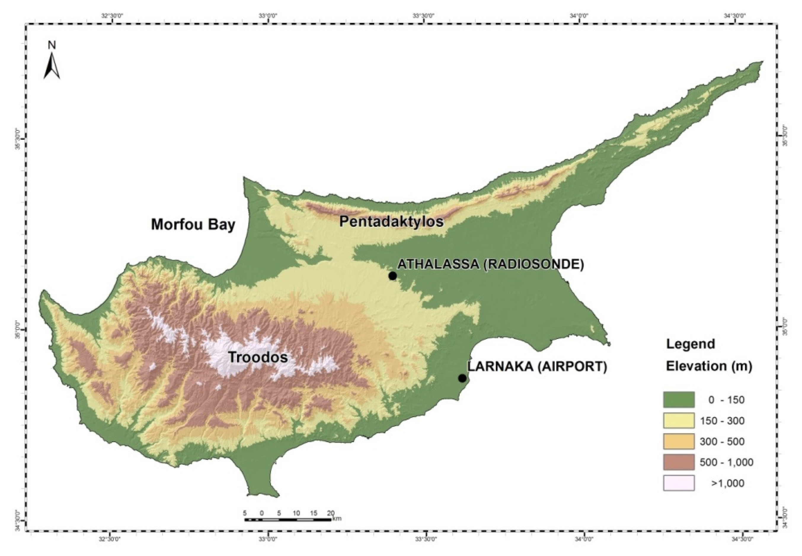
Figure 1.
Map of Cyprus showing the location of Athalassa actinometric station.
Figure 1.
Map of Cyprus showing the location of Athalassa actinometric station.
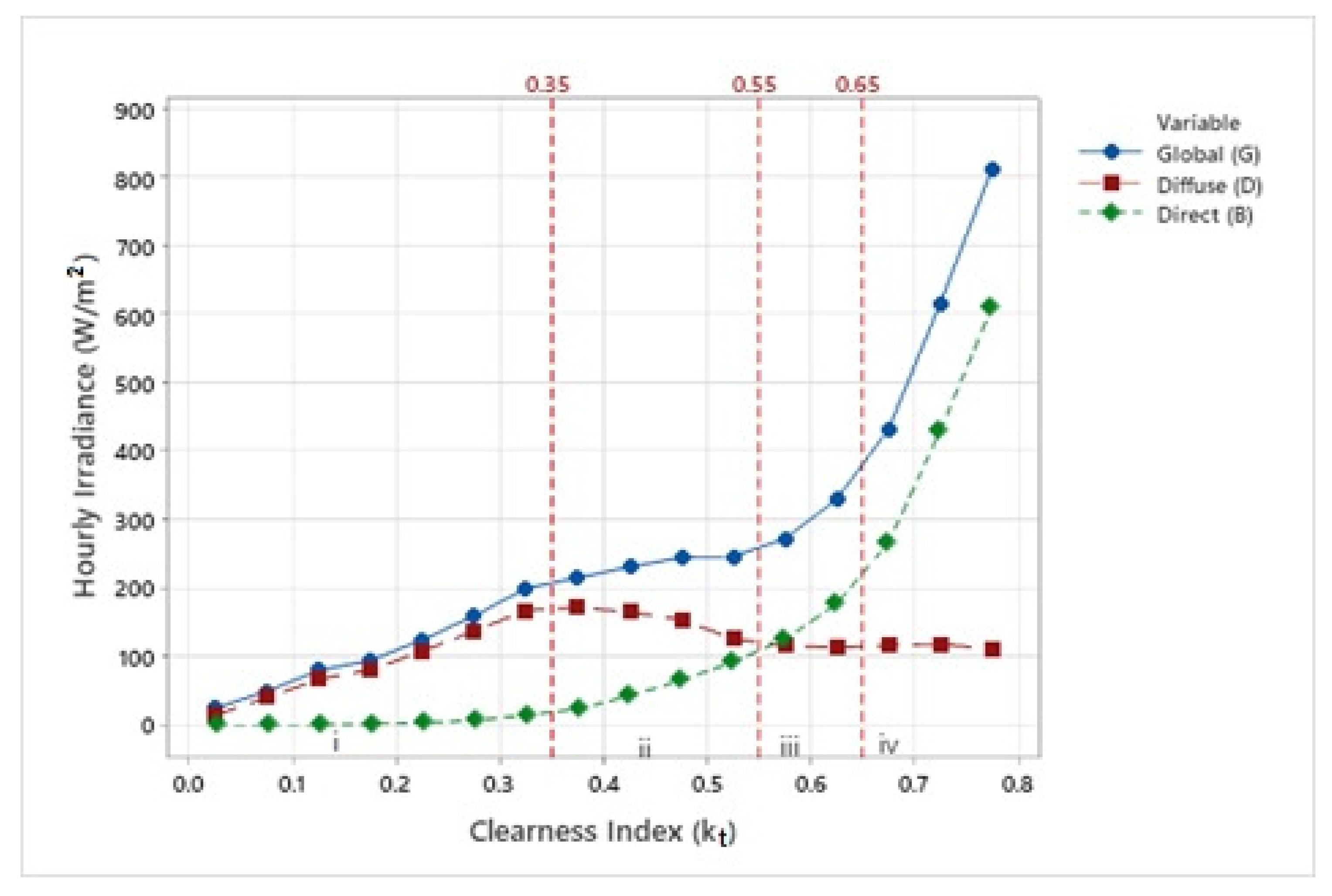
Figure 2.
Block-average values of global, diffuse and direct components of solar radiation, at the surface, in terms of clearness index intervals. Vertical dashed lines define regions of kt values associated to sky conditions and identified by i (cloudy sky), ii (partially cloudy with predominance of diffuse component), iii (partially cloudy with predominance of direct component) and iv (clear sky) interval.
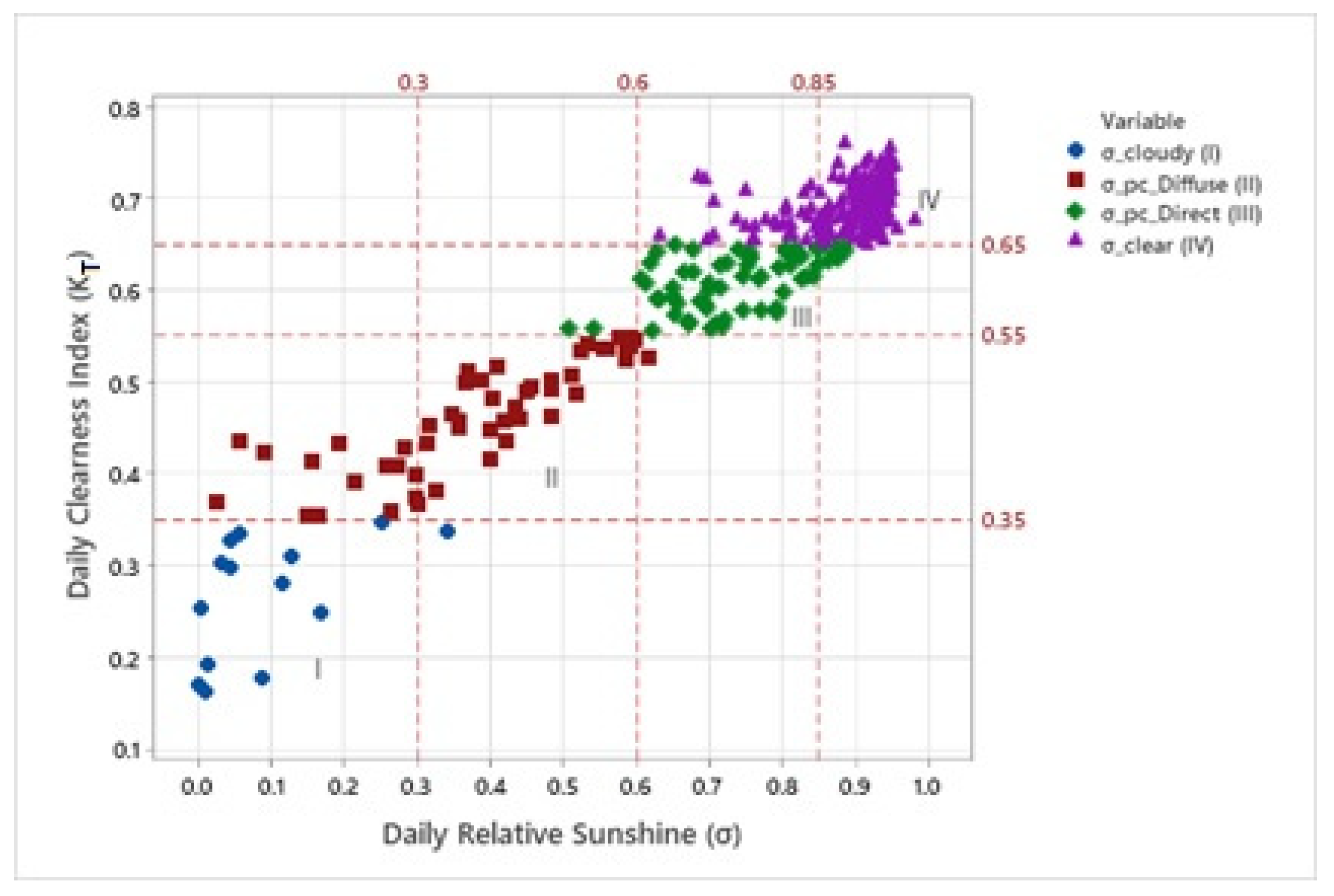
Figure 3.
Relationship between the daily clearness index (KT) and relative sunshine duration (σ) which define the four classes of sky conditions.
Figure 3.
Relationship between the daily clearness index (KT) and relative sunshine duration (σ) which define the four classes of sky conditions.
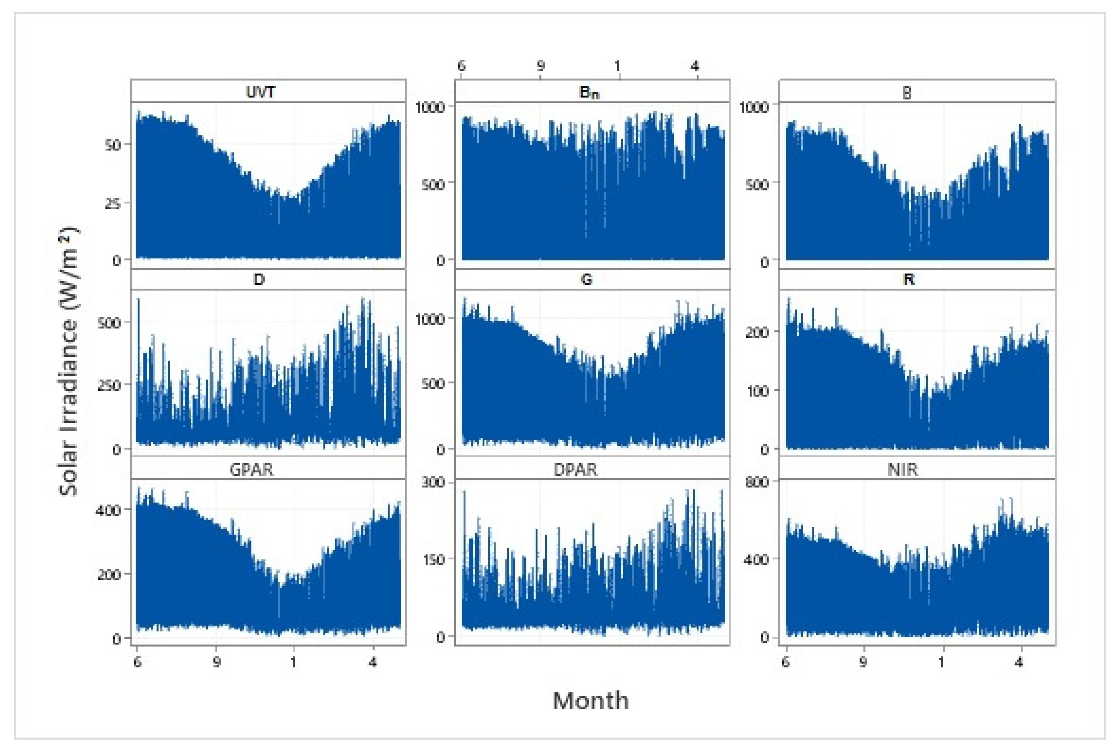
Figure 4.
Time series plots of solar shortwave radiation components during the period June 2020–May 2021.
Figure 4.
Time series plots of solar shortwave radiation components during the period June 2020–May 2021.
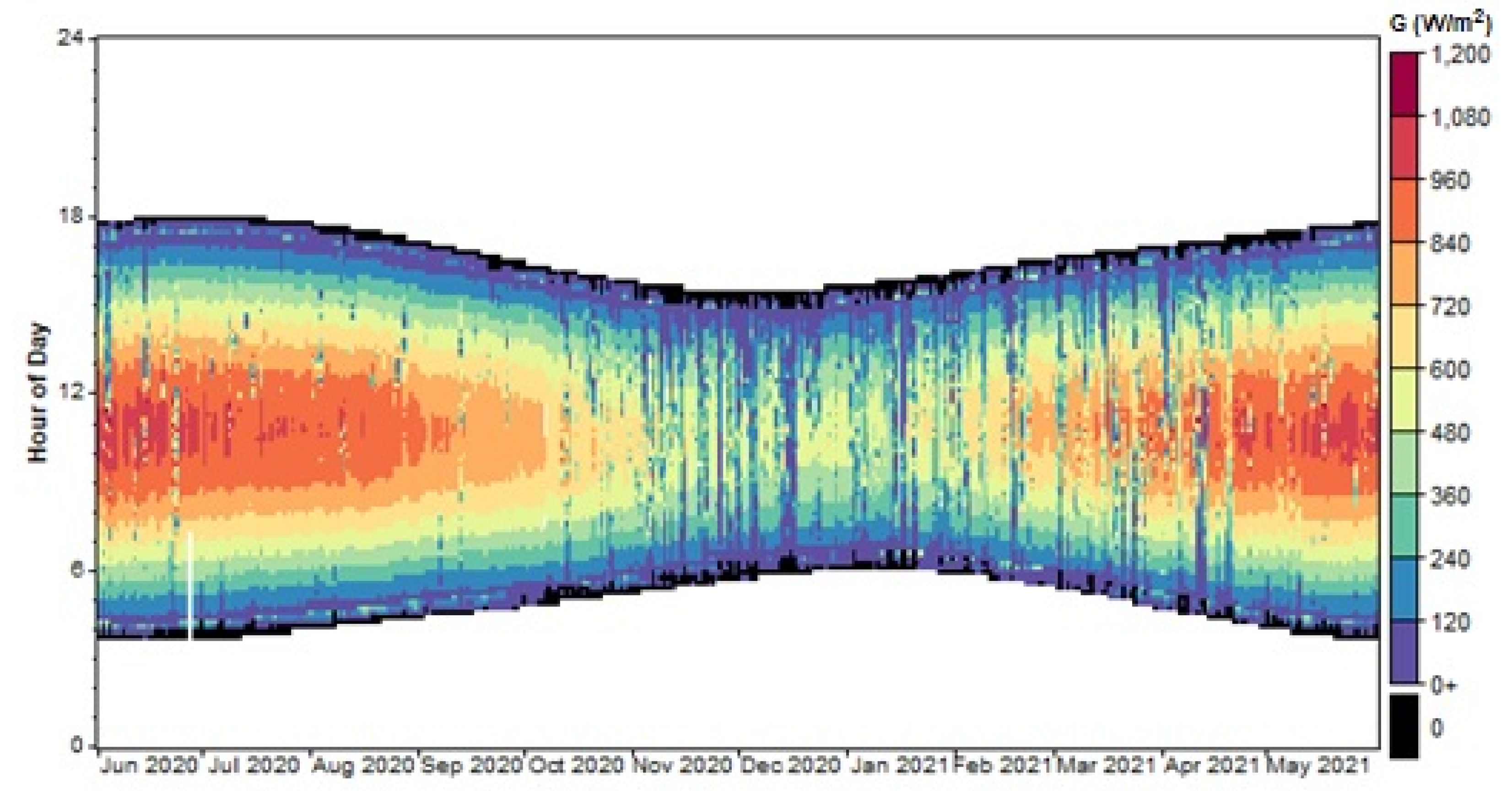
Figure 5.
Two-dimensional representation of global radiation (G).
Figure 5.
Two-dimensional representation of global radiation (G).
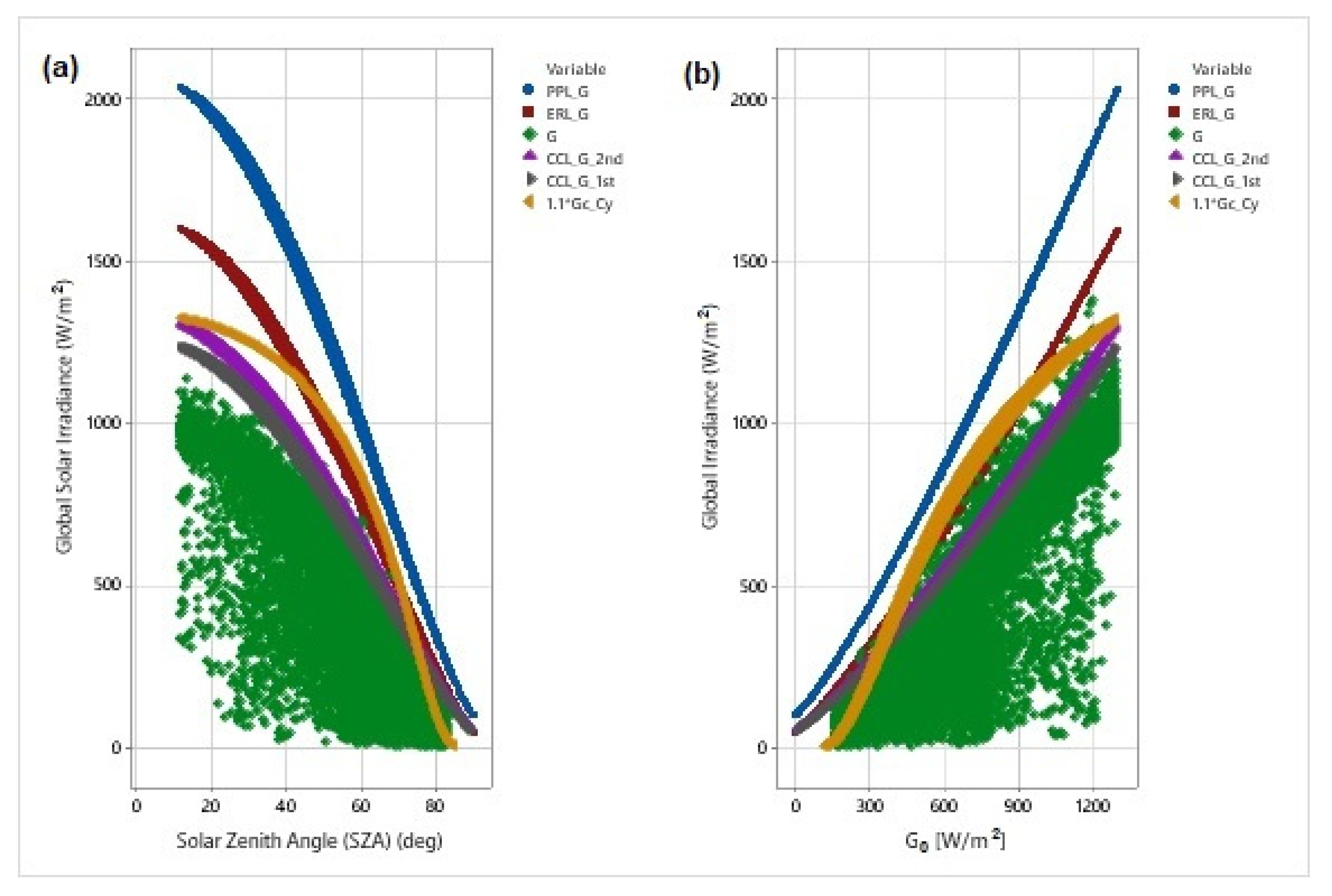
Figure 6.
(a) graphical representation of PPL, ERL and CCL tests of the average 10 min irradiances of the pyranometer on solar tracker (G) as a function of solar zenith angle (SZA); and (b) graphical representation of PPL, ERL and CCL tests of the maximum 10 min irradiances of the pyranometer on solar tracker (G) as a function of extraterrestrial irradiance at the top of the atmosphere (G0).
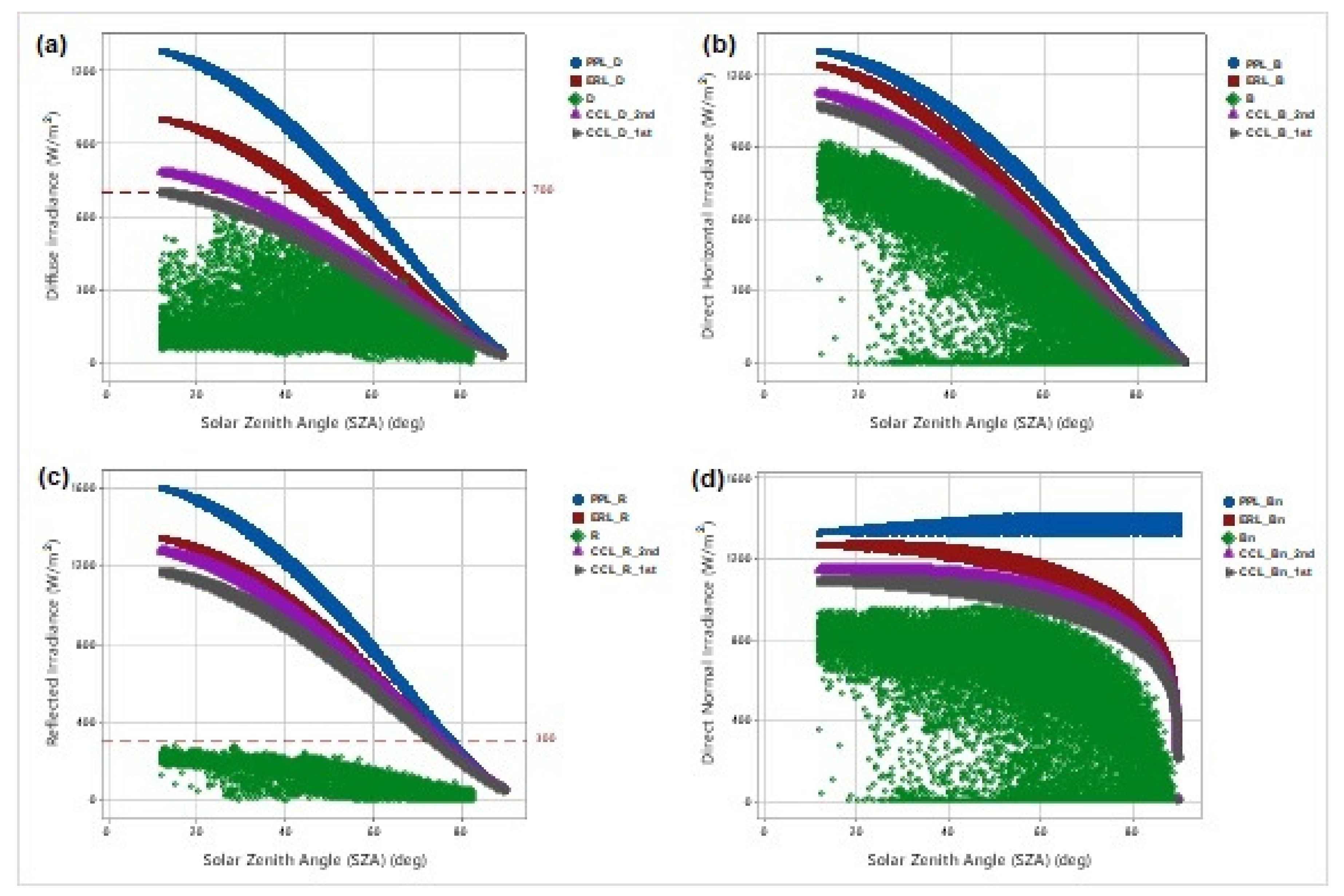
Figure 7.
Graphical representation of PPL, ERL and CCL tests of the average 10 min irradiances of: (a) the diffuse on solar tracker (D); (b) direct horizontal (B); (c) reflected (R); and (d) direct normal irradiance as a function of solar zenith angle (SZA).
Figure 7.
Graphical representation of PPL, ERL and CCL tests of the average 10 min irradiances of: (a) the diffuse on solar tracker (D); (b) direct horizontal (B); (c) reflected (R); and (d) direct normal irradiance as a function of solar zenith angle (SZA).
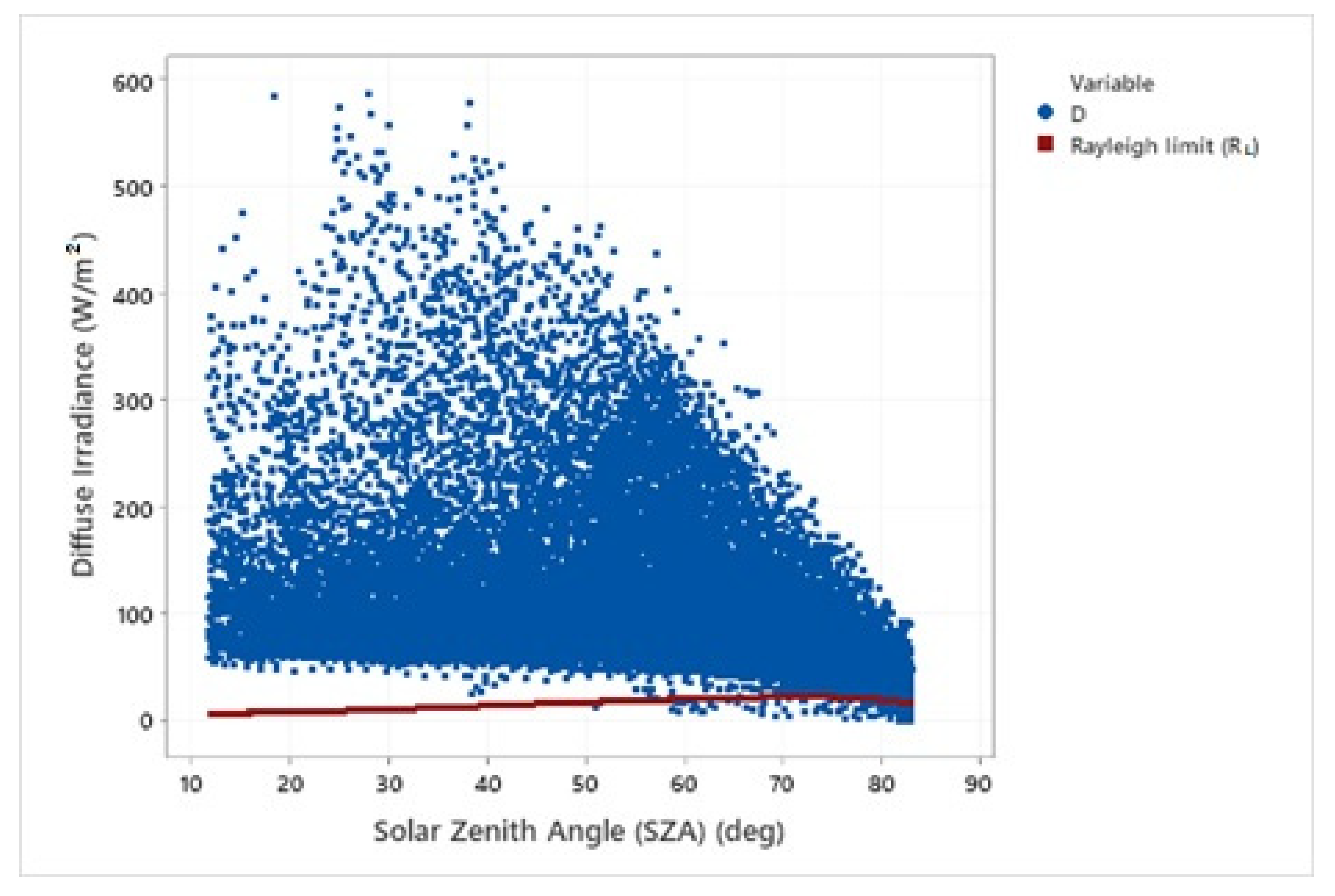
Figure 8.
Comparison based on the Rayleigh limit for data points that have kd < 0.8 and G > 500 W/m2.
Figure 8.
Comparison based on the Rayleigh limit for data points that have kd < 0.8 and G > 500 W/m2.
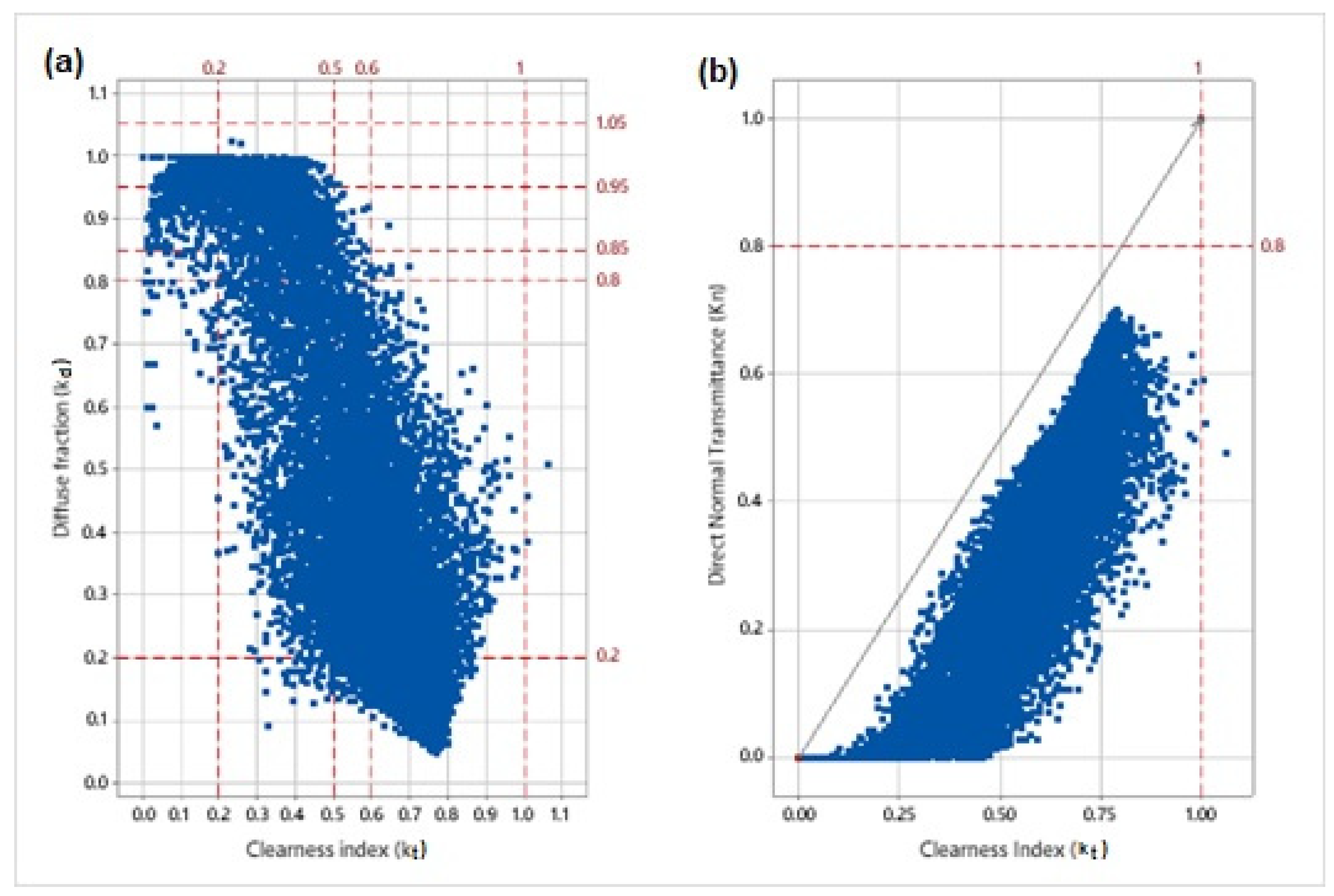
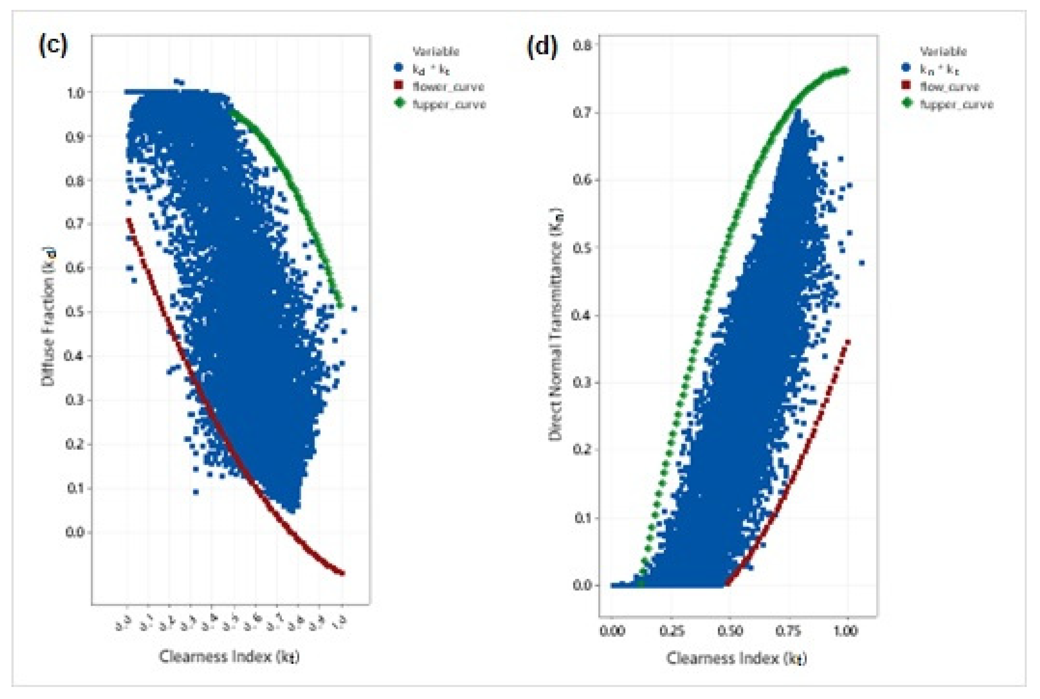
Figure 9.
Scatter plot of 10-min values in: (a) kd-kt space and (b) kn-kt space and limits for quality control tests. Scatter plot of 10-min values in (c) kd-kt space and (d) kn-kt space and limits for quality control tests.
Figure 9.
Scatter plot of 10-min values in: (a) kd-kt space and (b) kn-kt space and limits for quality control tests. Scatter plot of 10-min values in (c) kd-kt space and (d) kn-kt space and limits for quality control tests.
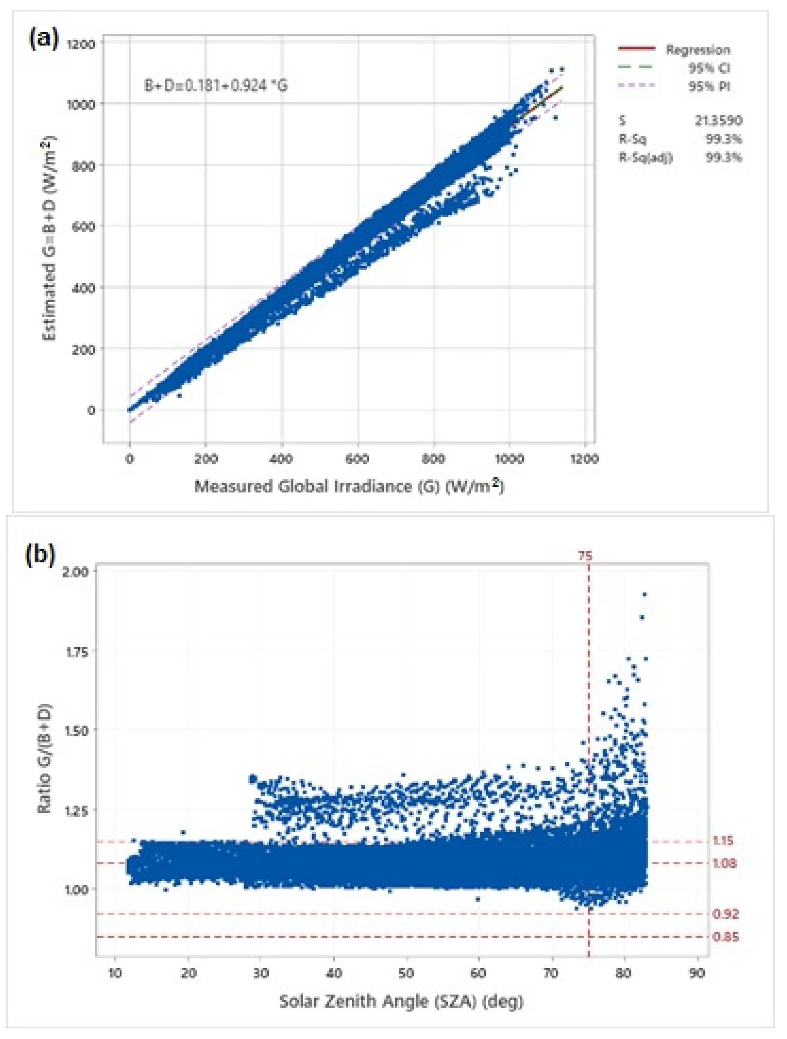
Figure 10.
(a) linear regression of the estimated sum of the measured irradiances (B + D) and the relevant global irradiances (G); and (b) Ratio of G/(B + D) as a function of solar zenith angle (SZA) with the reference lines within the ratio should be detected.
Figure 10.
(a) linear regression of the estimated sum of the measured irradiances (B + D) and the relevant global irradiances (G); and (b) Ratio of G/(B + D) as a function of solar zenith angle (SZA) with the reference lines within the ratio should be detected.
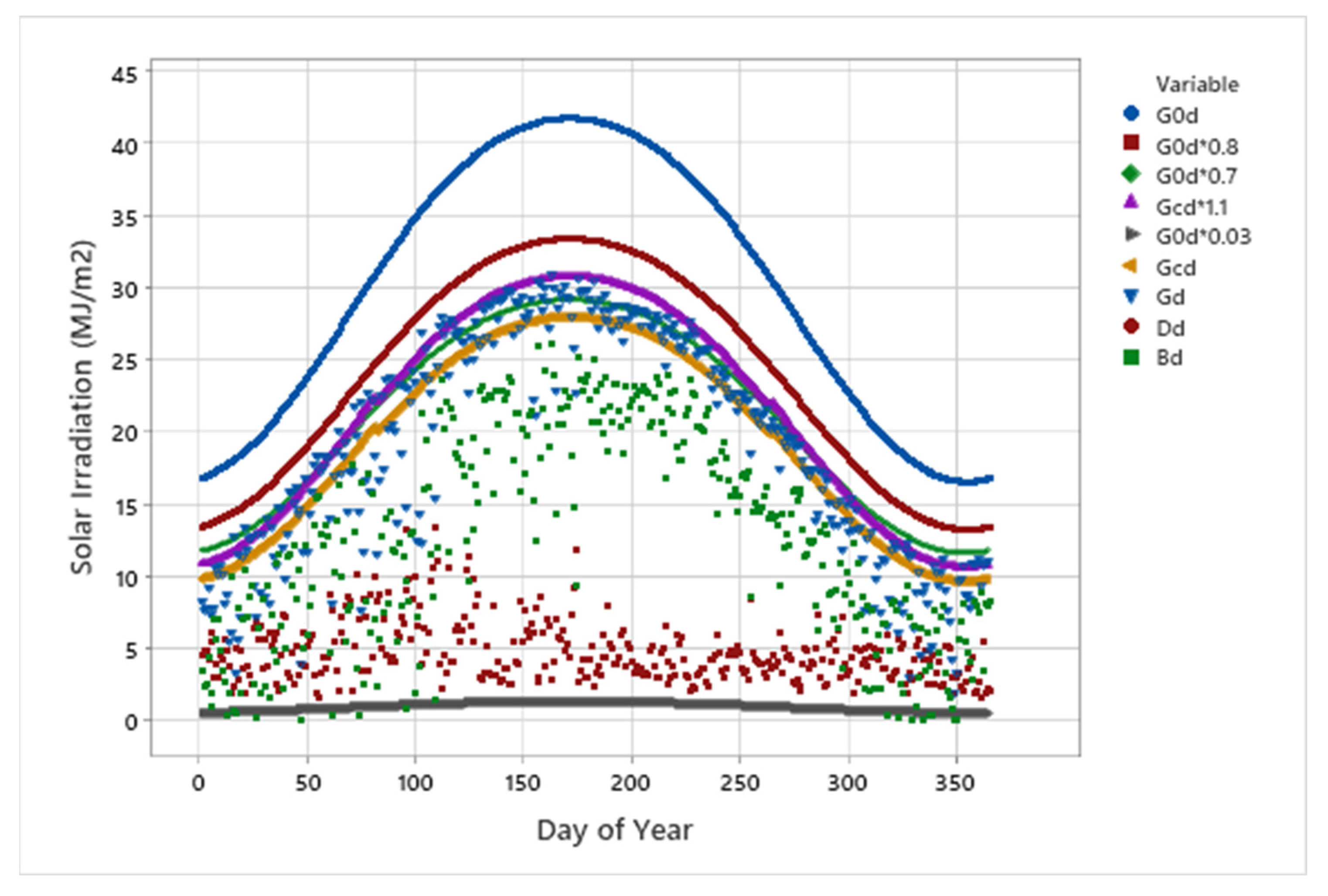
Figure 11.
Daily totals of global irradiation (Gd) compared to the respective extraterrestrial (G0d) and clear-sky irradiation (Gcd). The daily totals of horizontal direct (Bd) and diffuse irradiation (Dd) are also shown in the graph.
Figure 11.
Daily totals of global irradiation (Gd) compared to the respective extraterrestrial (G0d) and clear-sky irradiation (Gcd). The daily totals of horizontal direct (Bd) and diffuse irradiation (Dd) are also shown in the graph.
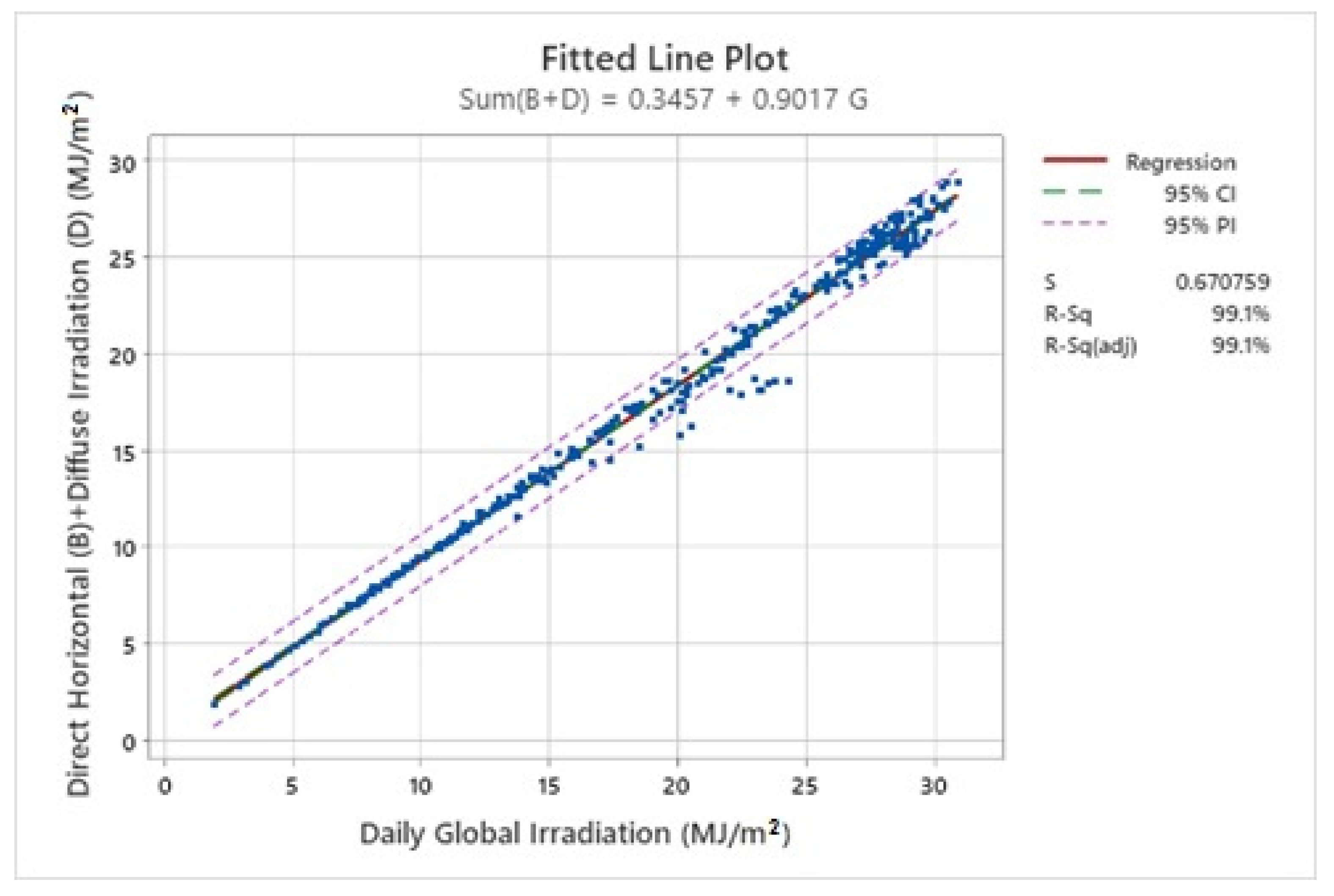
Figure 12.
Linear regression between the sum (Bd + Dd) and global irradiation (Gd).
Figure 12.
Linear regression between the sum (Bd + Dd) and global irradiation (Gd).
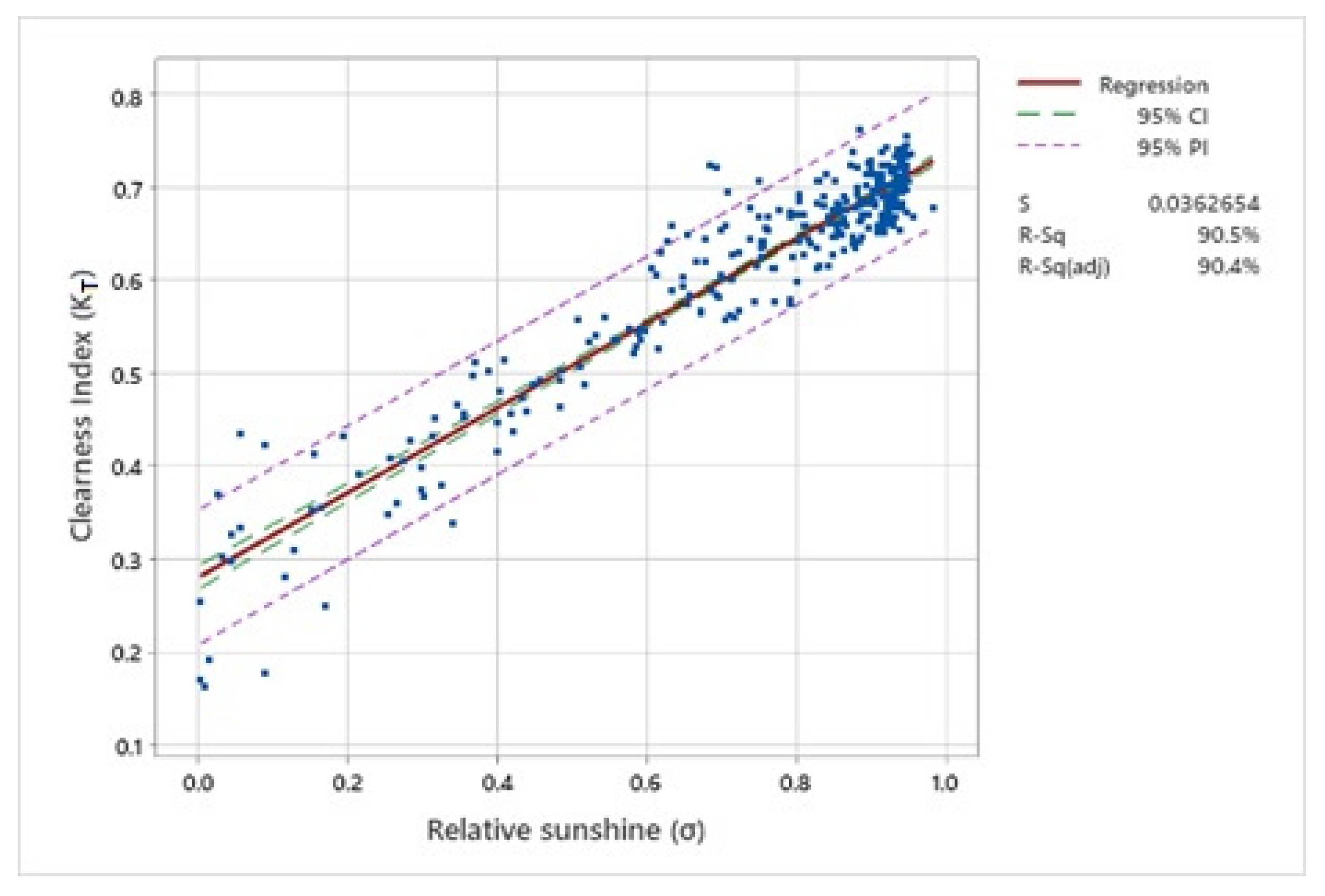
Figure 13.
Linear relationship between KT and σ. ,
.
Figure 13.
Linear relationship between KT and σ. ,
.
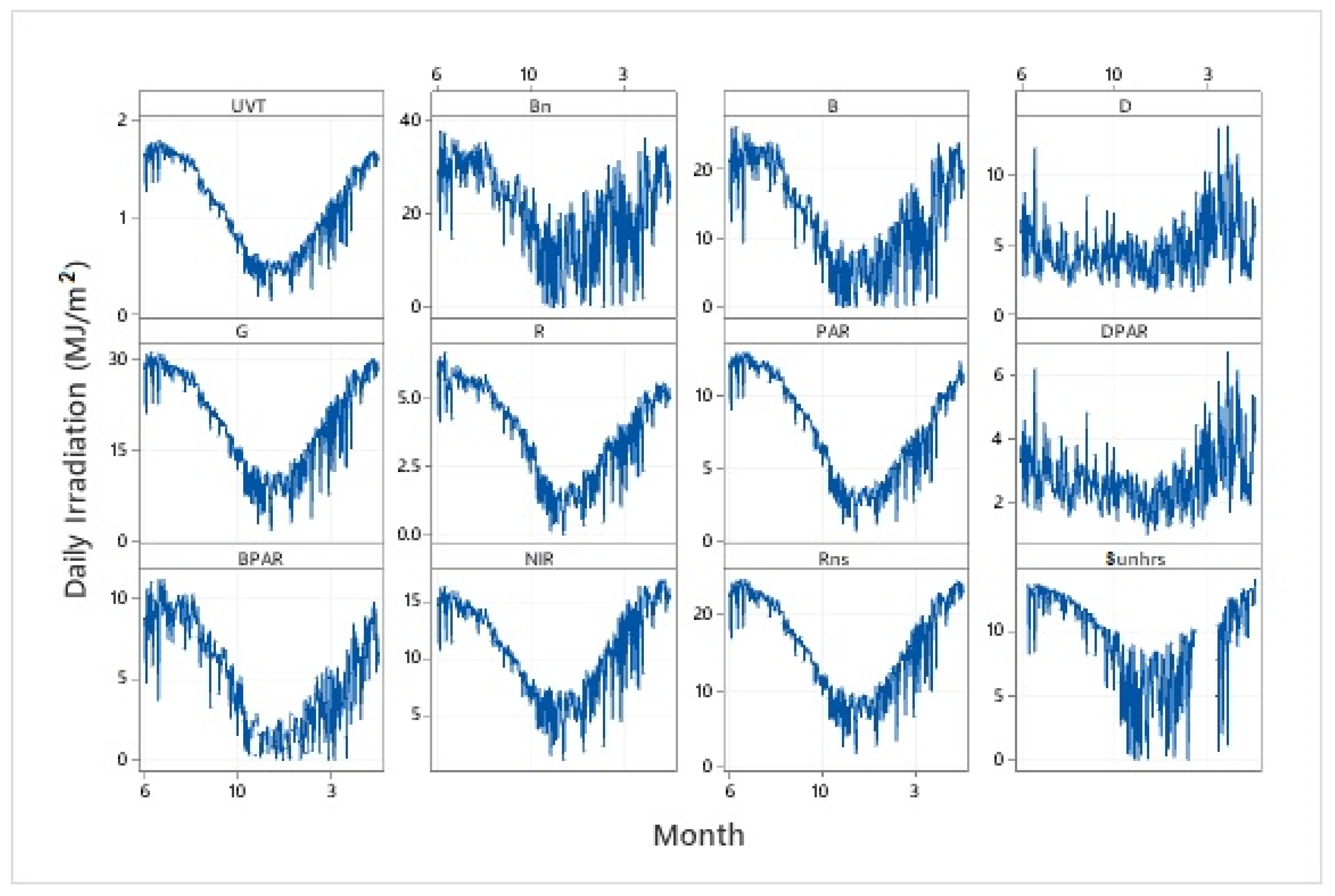
Figure 14.
Time series plots of daily values of all shortwave radiation components including daily sunshine duration.
Figure 14.
Time series plots of daily values of all shortwave radiation components including daily sunshine duration.
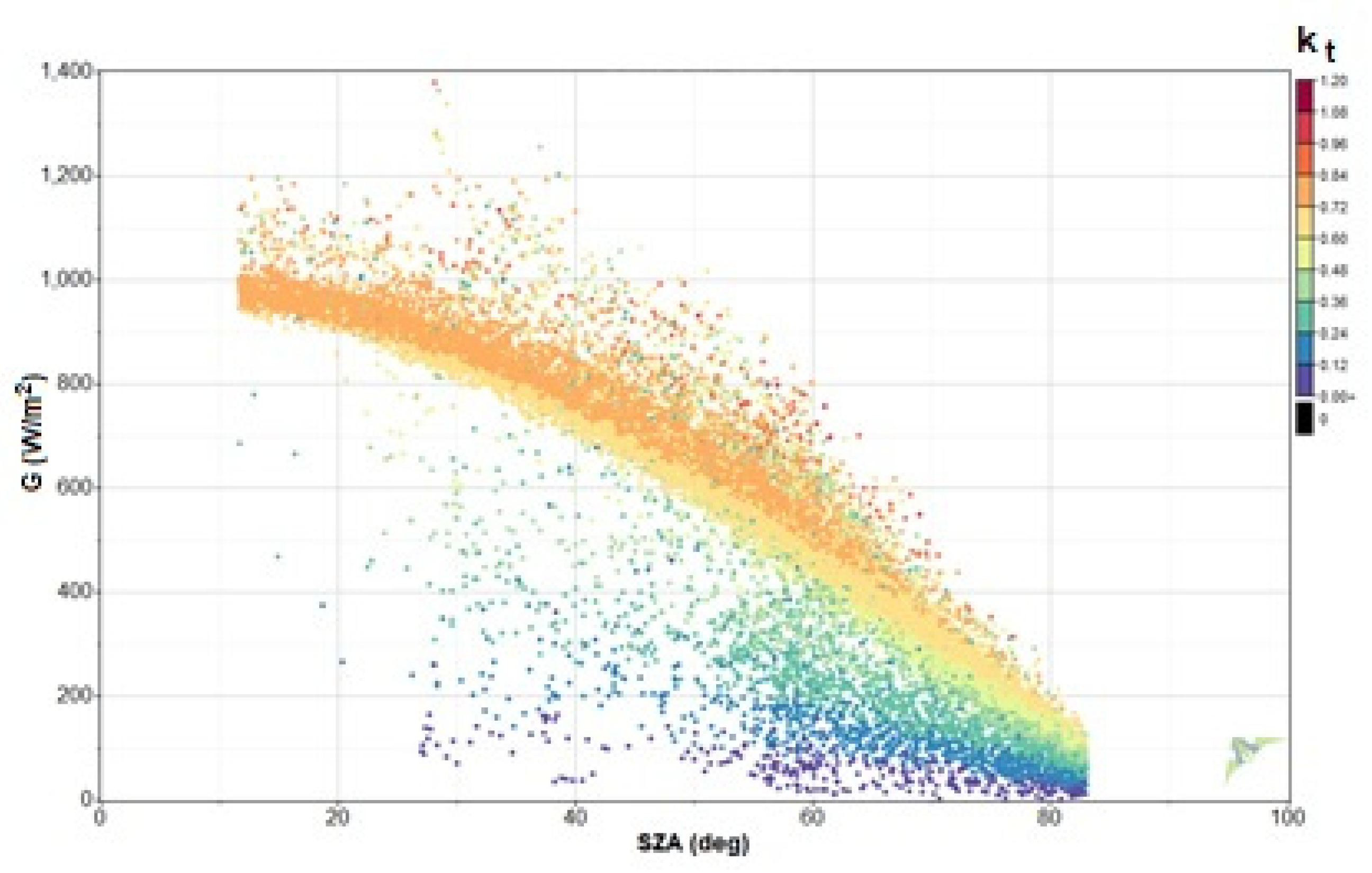
Figure 15.
Solar global irradiances as a function of solar zenith angle (SZA) and clearness index (kt).
Figure 15.
Solar global irradiances as a function of solar zenith angle (SZA) and clearness index (kt).
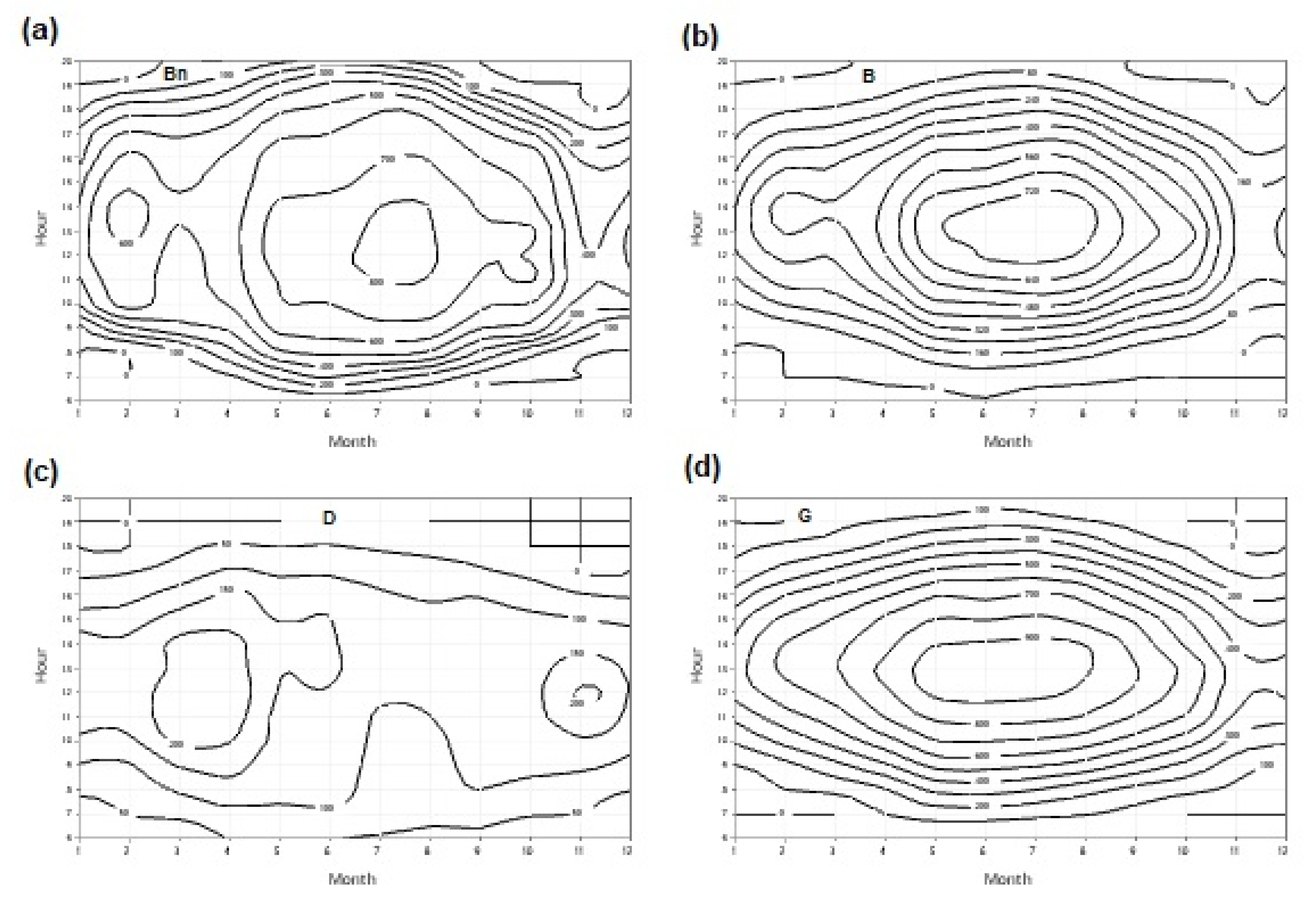
Figure 16.
Isoline diagrams of monthly mean hourly: (a) direct normal; (b) direct horizontal; (c) diffuse; and (d) global irradiance values (W/m2).
Figure 16.
Isoline diagrams of monthly mean hourly: (a) direct normal; (b) direct horizontal; (c) diffuse; and (d) global irradiance values (W/m2).
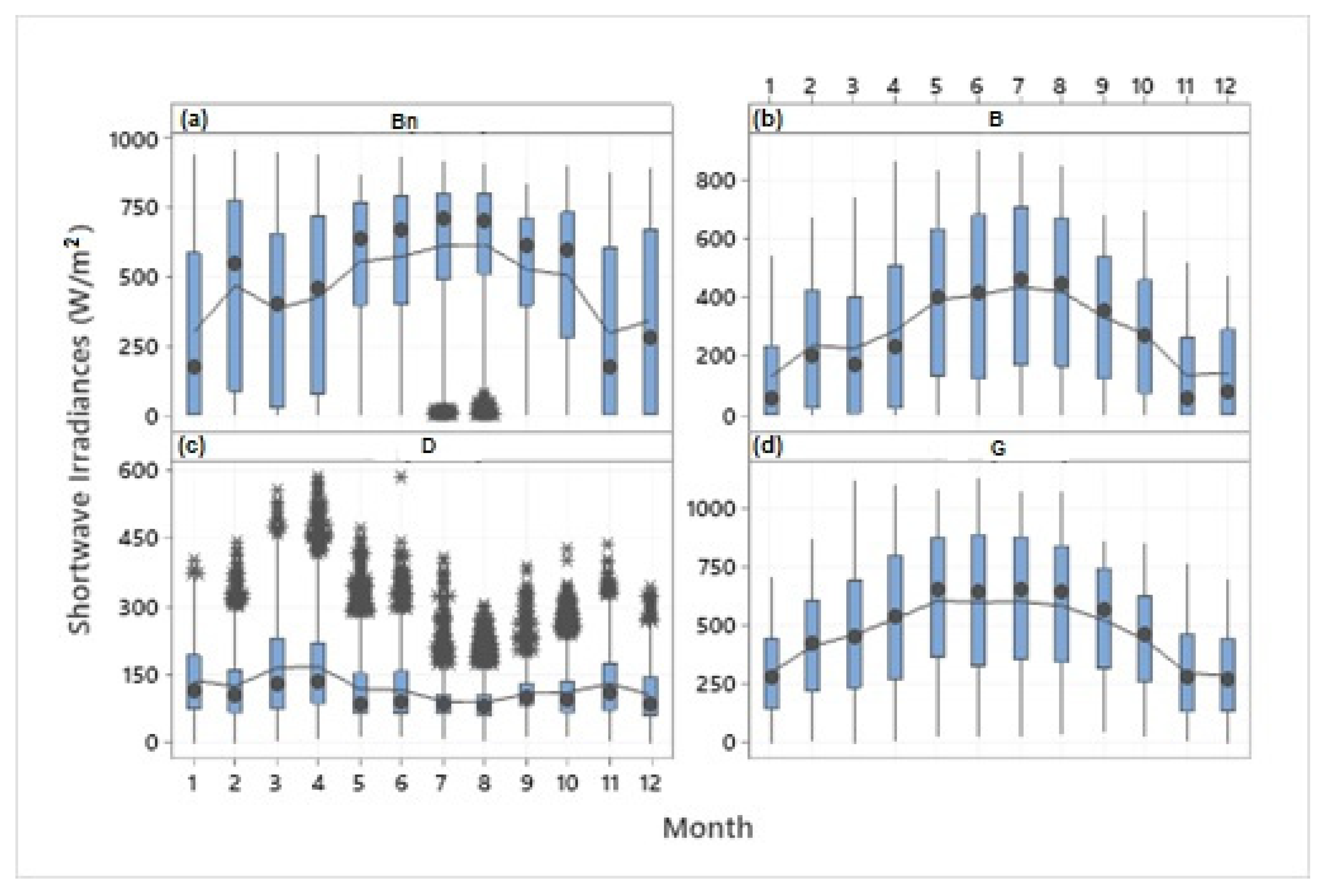
Figure 17.
Boxplots of irradiances of the shortwave radiation components: (a) direct normal (Bn); (b) direct horizontal (B); (c) diffuse (D); and (d) global (G). The symbol of median values is represented as circle in the boxplot. The asterisks denote the outliers. The smooth curve represents the mean values of each month of the year.
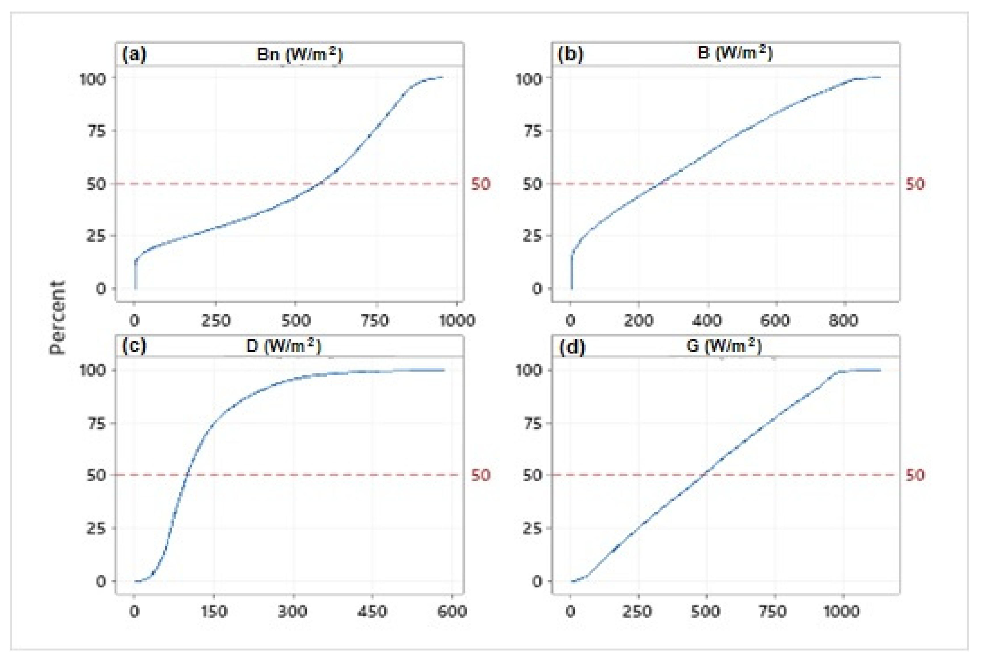
Figure 18.
Cumulative frequency distribution (CDF) of shortwave solar radiation components: (a) direct normal (Bn); (b) direct horizontal (B); (c) diffuse (D); and (d) global (G) irradiances (W/m2).
Figure 18.
Cumulative frequency distribution (CDF) of shortwave solar radiation components: (a) direct normal (Bn); (b) direct horizontal (B); (c) diffuse (D); and (d) global (G) irradiances (W/m2).
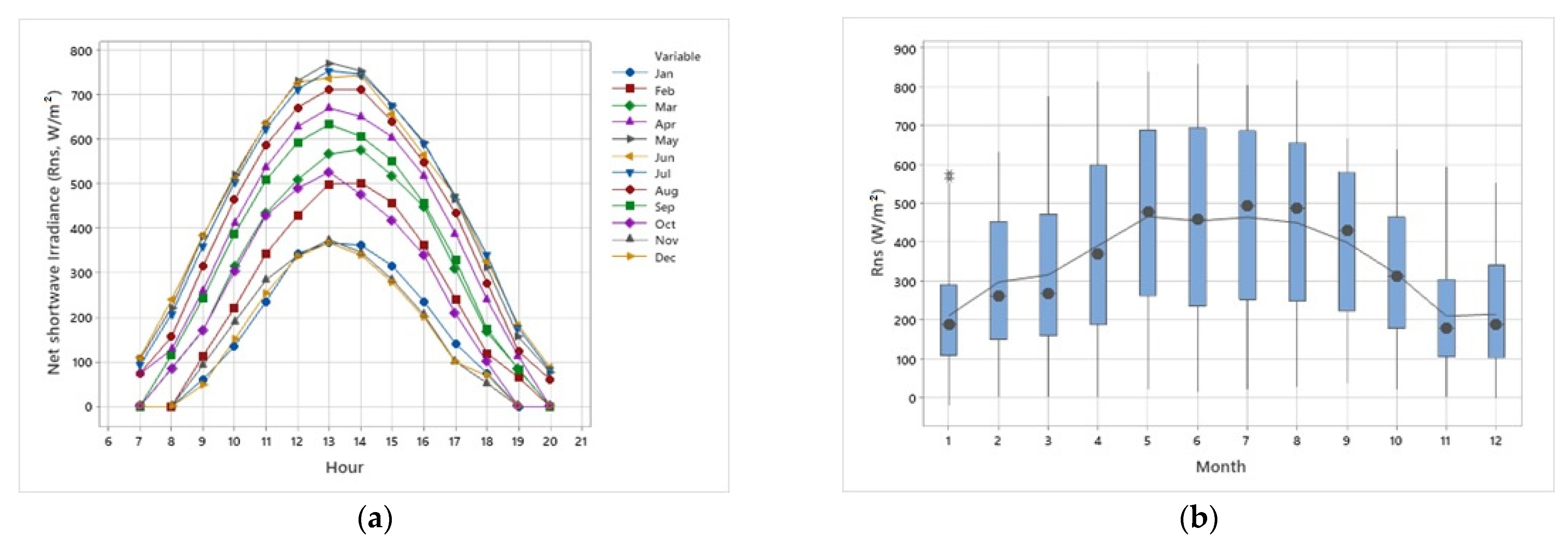
Figure 19.
(a) diurnal variation of the average hourly values of Rns for each month of the year; and (b) monthly variability of net shortwave irradiances (W/m2). Symbol * indicates an outlier.
Figure 19.
(a) diurnal variation of the average hourly values of Rns for each month of the year; and (b) monthly variability of net shortwave irradiances (W/m2). Symbol * indicates an outlier.
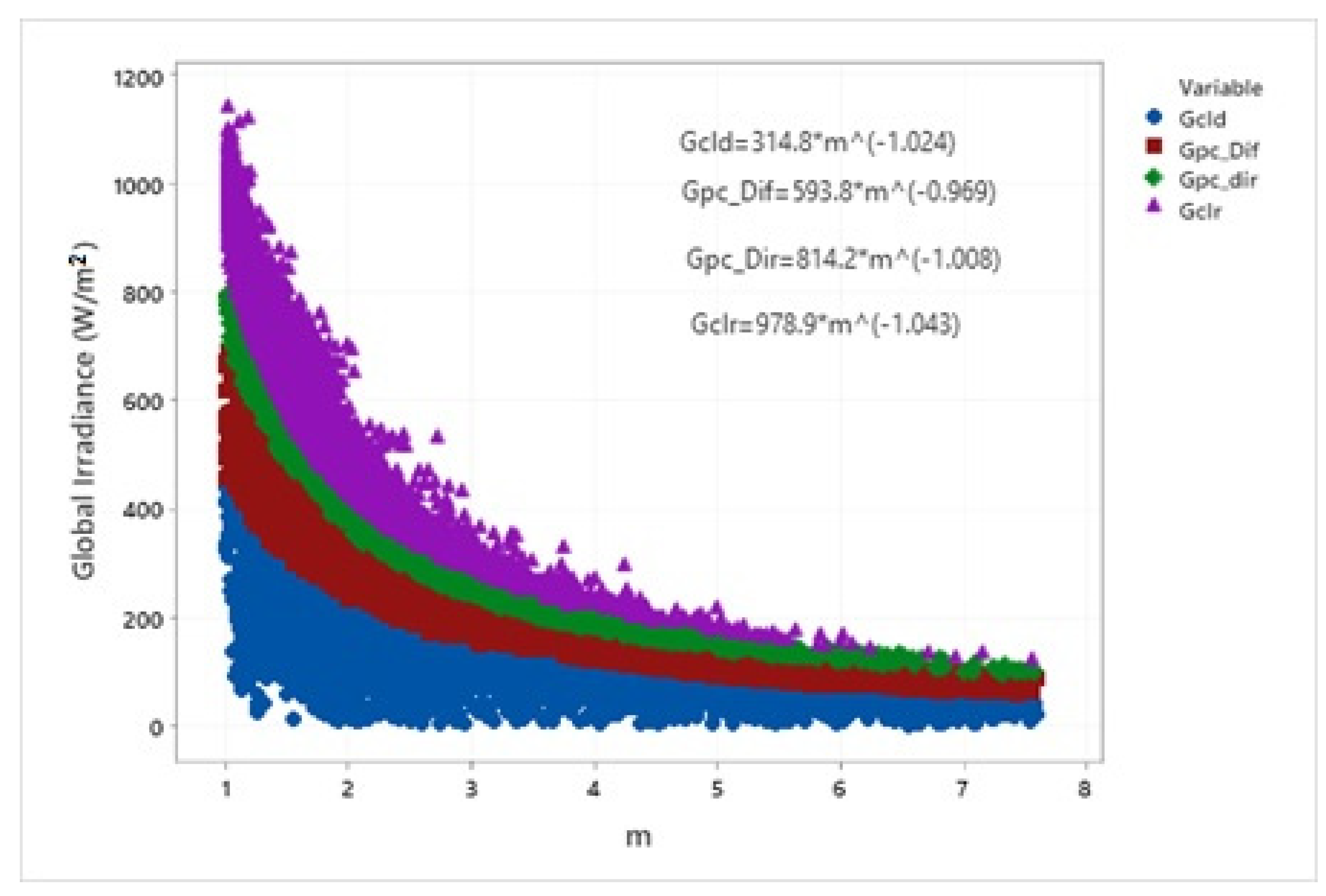
Figure 20.
Relationship of global irradiance in W/m2 and optical air mass (m).
Figure 20.
Relationship of global irradiance in W/m2 and optical air mass (m).
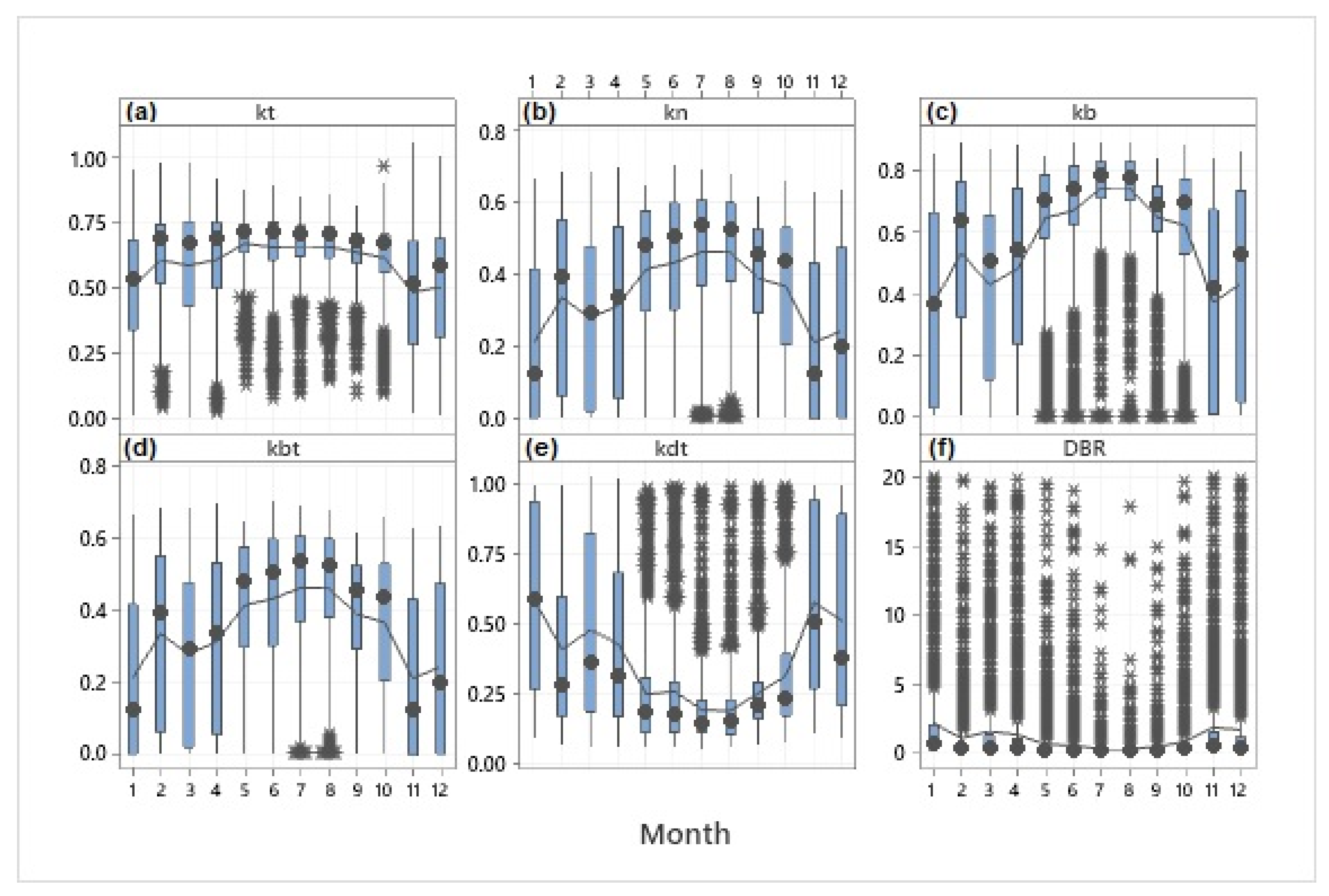
Figure 21.
Monthly boxplots of: (a) clearness index (kt); (b) clearness index of direct normal irradiance (kn); (c) direct horizontal fraction (kb); (d) direct clearness index (kbt); (e) diffuse fraction (kd); and (f) diffuse to beam ratio ().
Figure 21.
Monthly boxplots of: (a) clearness index (kt); (b) clearness index of direct normal irradiance (kn); (c) direct horizontal fraction (kb); (d) direct clearness index (kbt); (e) diffuse fraction (kd); and (f) diffuse to beam ratio ().
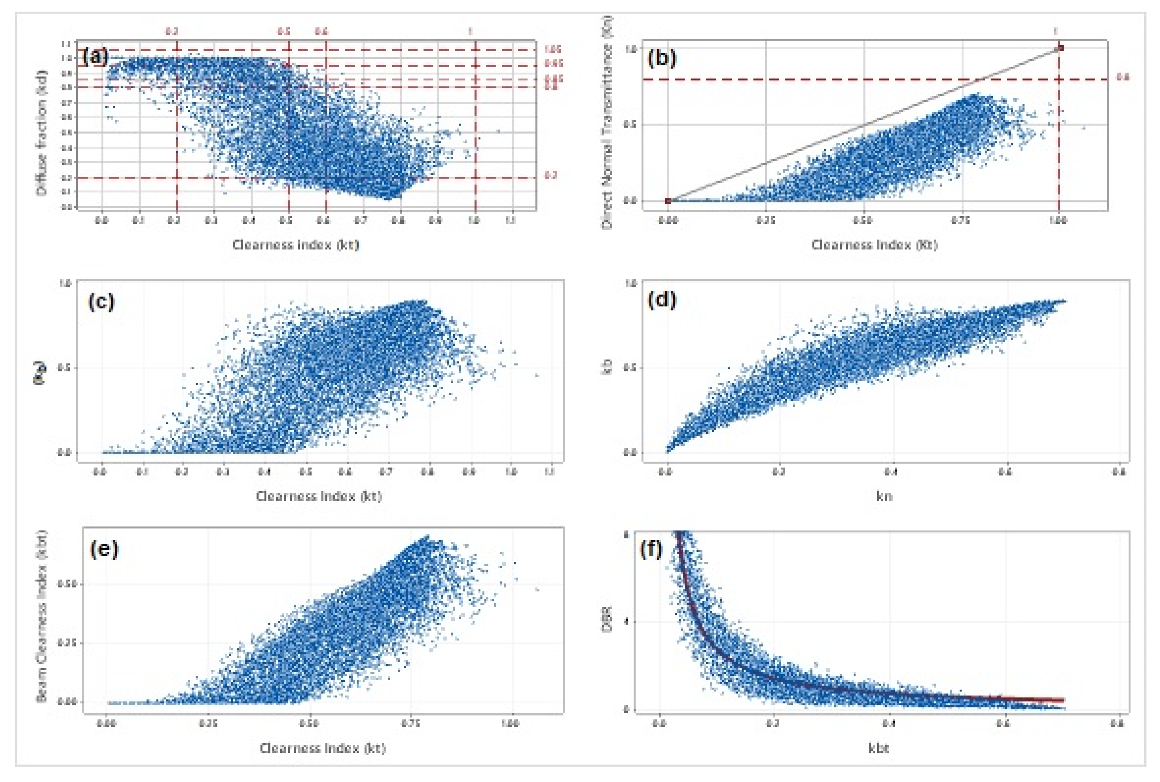
Figure 22.
(a) Diffuse fraction to global irradiance (kd); (b) direct normal transmittance (kn); (c) fraction of direct horizontal radiation to global irradiance (kb) as a function of clearness index (kt); (d) kb vs. kn; (e) kbt vs. kt; and (f) DBR vs. kbt.
Figure 22.
(a) Diffuse fraction to global irradiance (kd); (b) direct normal transmittance (kn); (c) fraction of direct horizontal radiation to global irradiance (kb) as a function of clearness index (kt); (d) kb vs. kn; (e) kbt vs. kt; and (f) DBR vs. kbt.
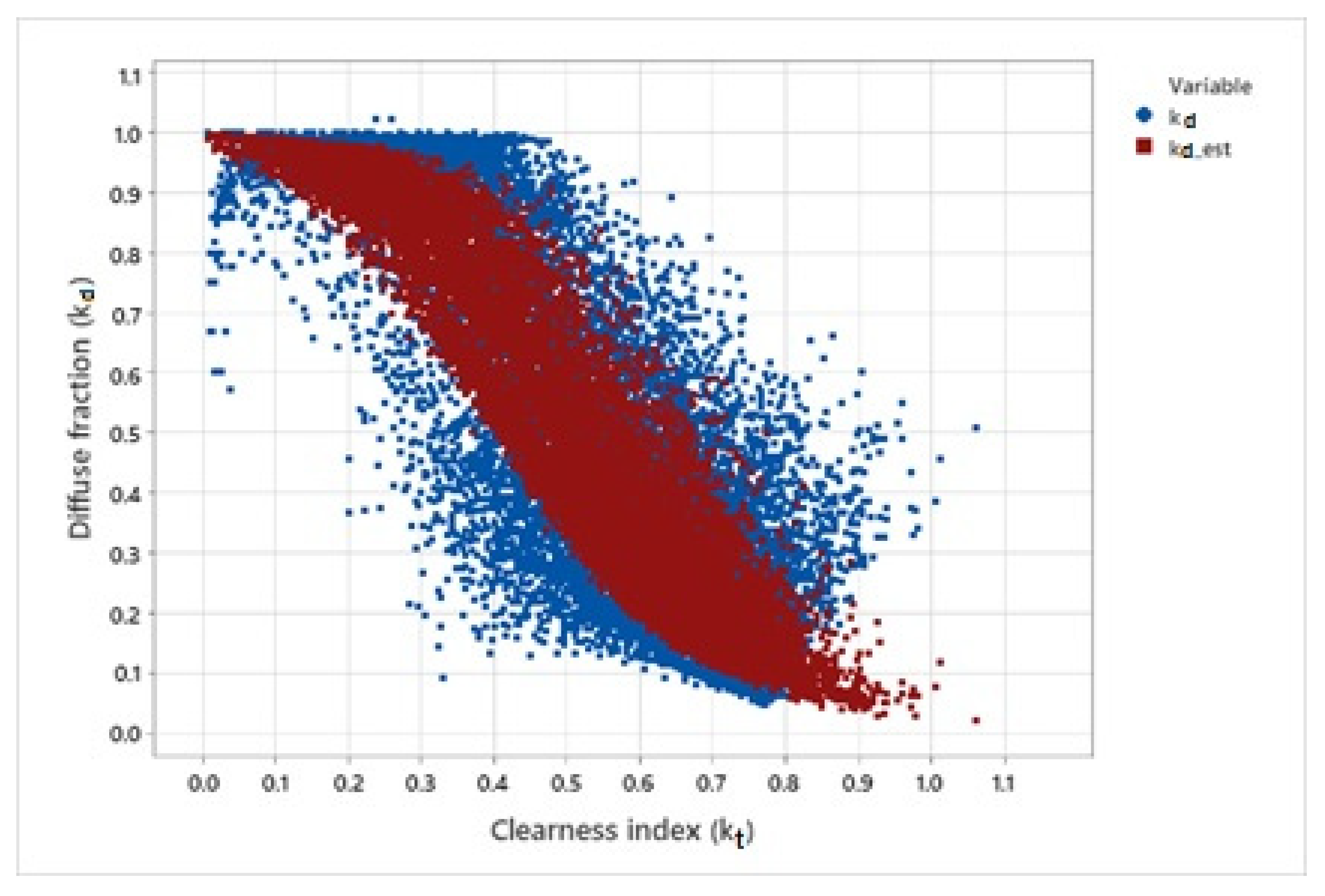
Figure 23.
The BRL diffuse fraction model fit with the clearness index (kt).
Figure 23.
The BRL diffuse fraction model fit with the clearness index (kt).
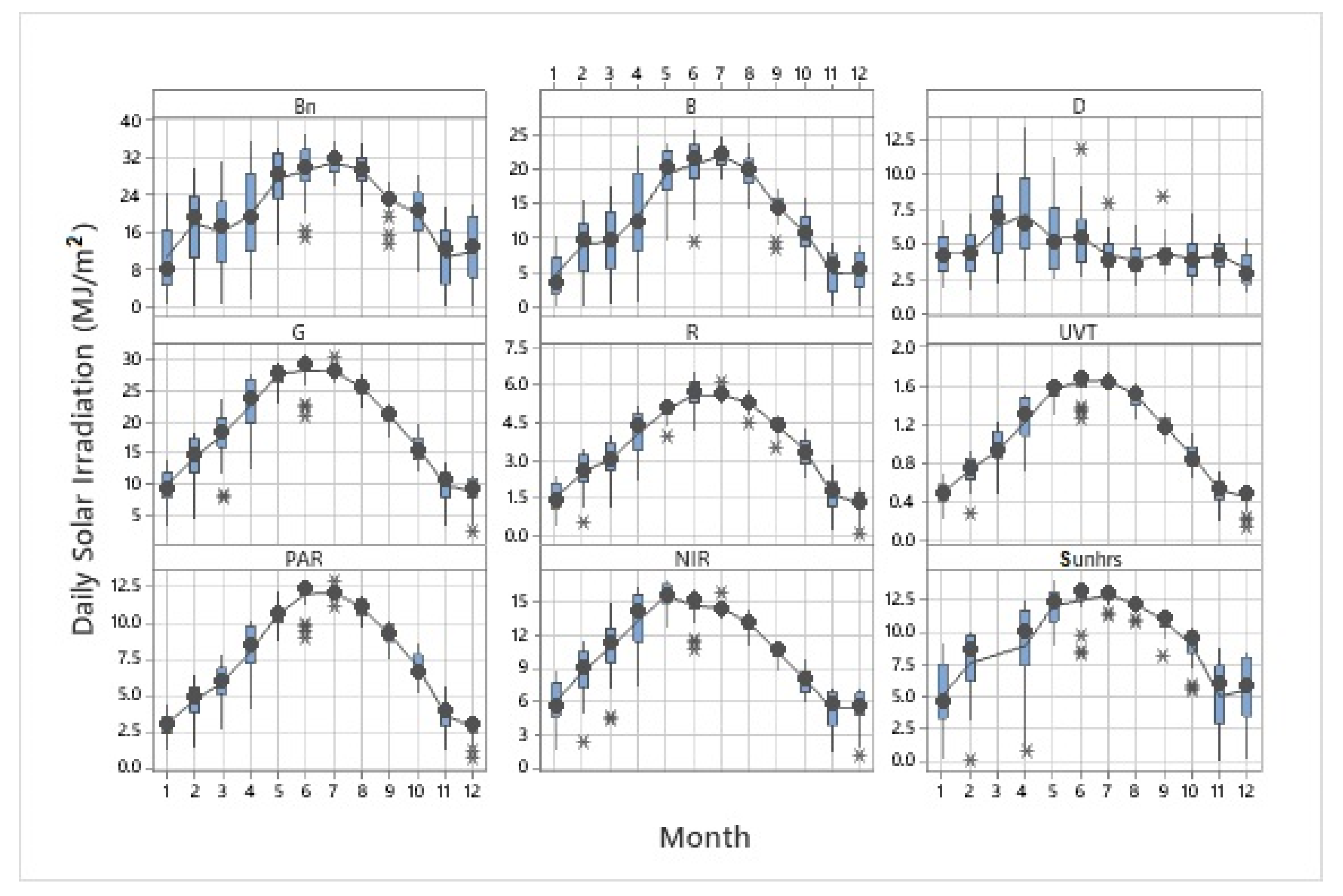
Figure 24.
Boxplots of daily solar irradiation (MJ/m2) of all radiation components. The smooth line represents the mean daily values of each month for each variable.
Figure 24.
Boxplots of daily solar irradiation (MJ/m2) of all radiation components. The smooth line represents the mean daily values of each month for each variable.
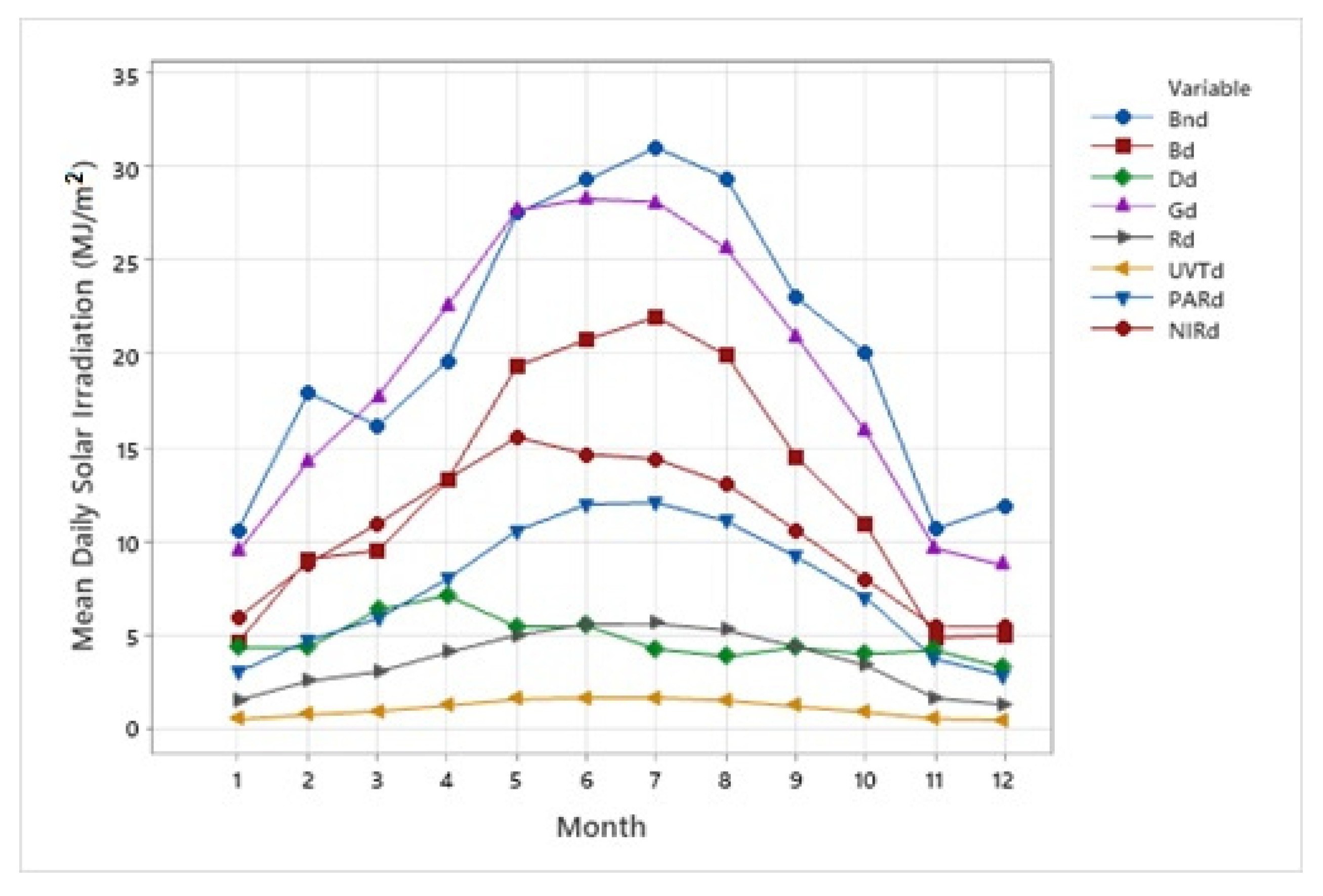
Figure 25.
Monthly mean daily values (MJ/m2) for all radiation components.
Figure 25.
Monthly mean daily values (MJ/m2) for all radiation components.
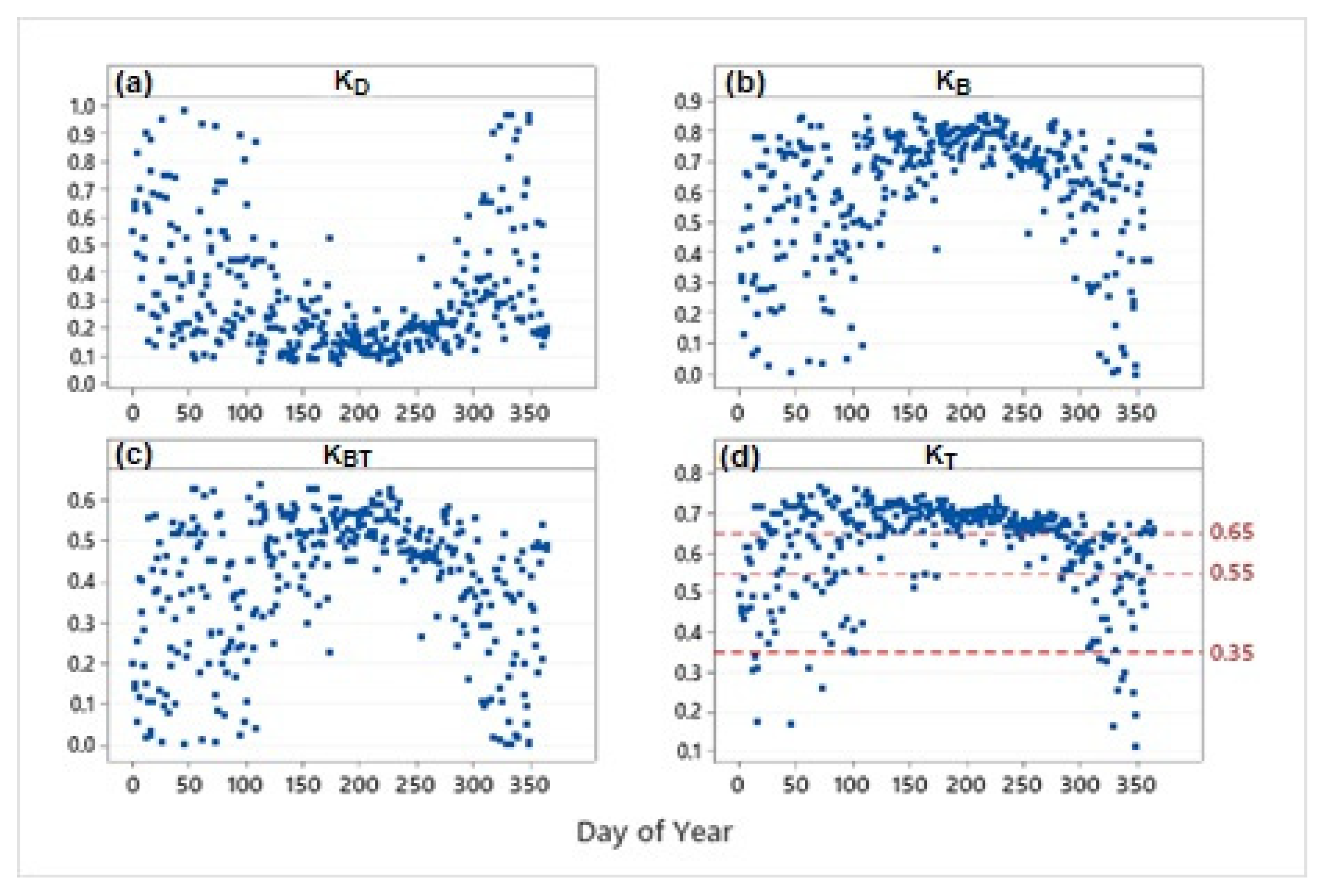
Figure 26.
Daily values of radiation indices: (a) diffuse fraction (KD); (b) direct horizontal fraction (KB); (c) direct clearness index (KBT); and (d) clearness index (KT), throughout the year.
Figure 26.
Daily values of radiation indices: (a) diffuse fraction (KD); (b) direct horizontal fraction (KB); (c) direct clearness index (KBT); and (d) clearness index (KT), throughout the year.
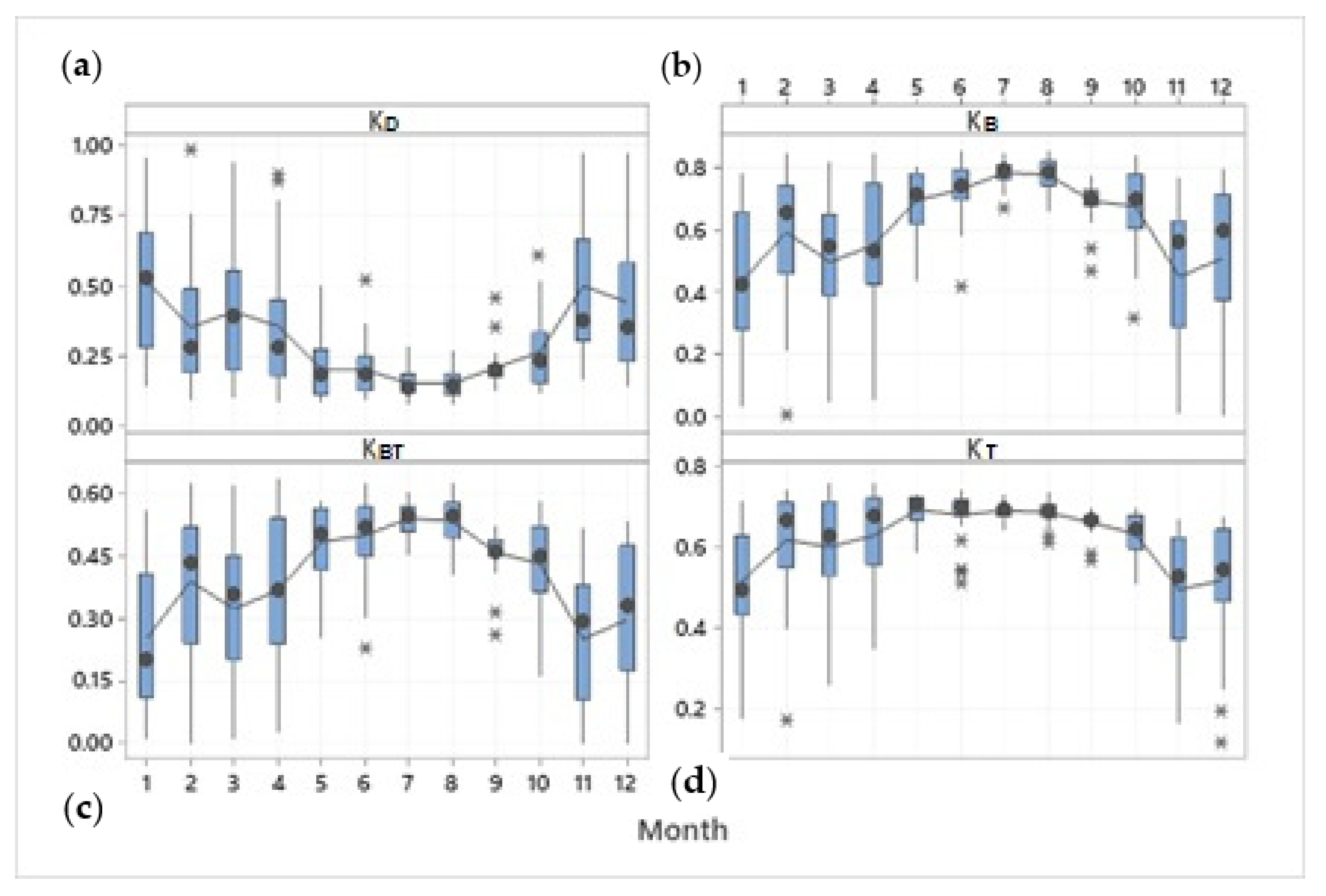
Figure 27.
Monthly boxplots for each daily radiation index: (a) diffuse fraction (KD); (b) direct horizontal fraction (KB); (c) direct clearness index (KBT); and (d) clearness index (KT).
Figure 27.
Monthly boxplots for each daily radiation index: (a) diffuse fraction (KD); (b) direct horizontal fraction (KB); (c) direct clearness index (KBT); and (d) clearness index (KT).
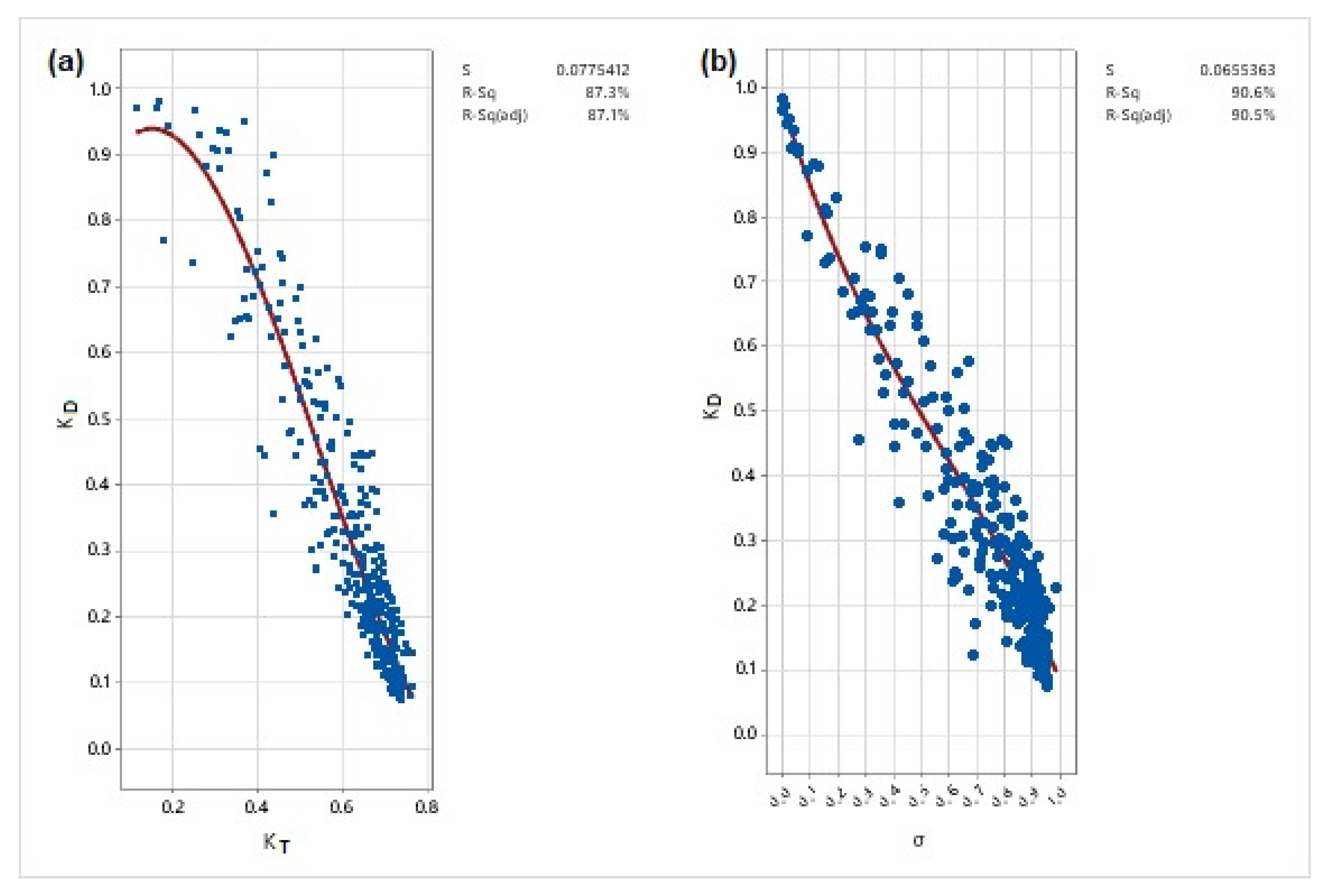
Figure 28.
(a) relation between KD and KT; and (b) relation between KD and σ.
Figure 28.
(a) relation between KD and KT; and (b) relation between KD and σ.
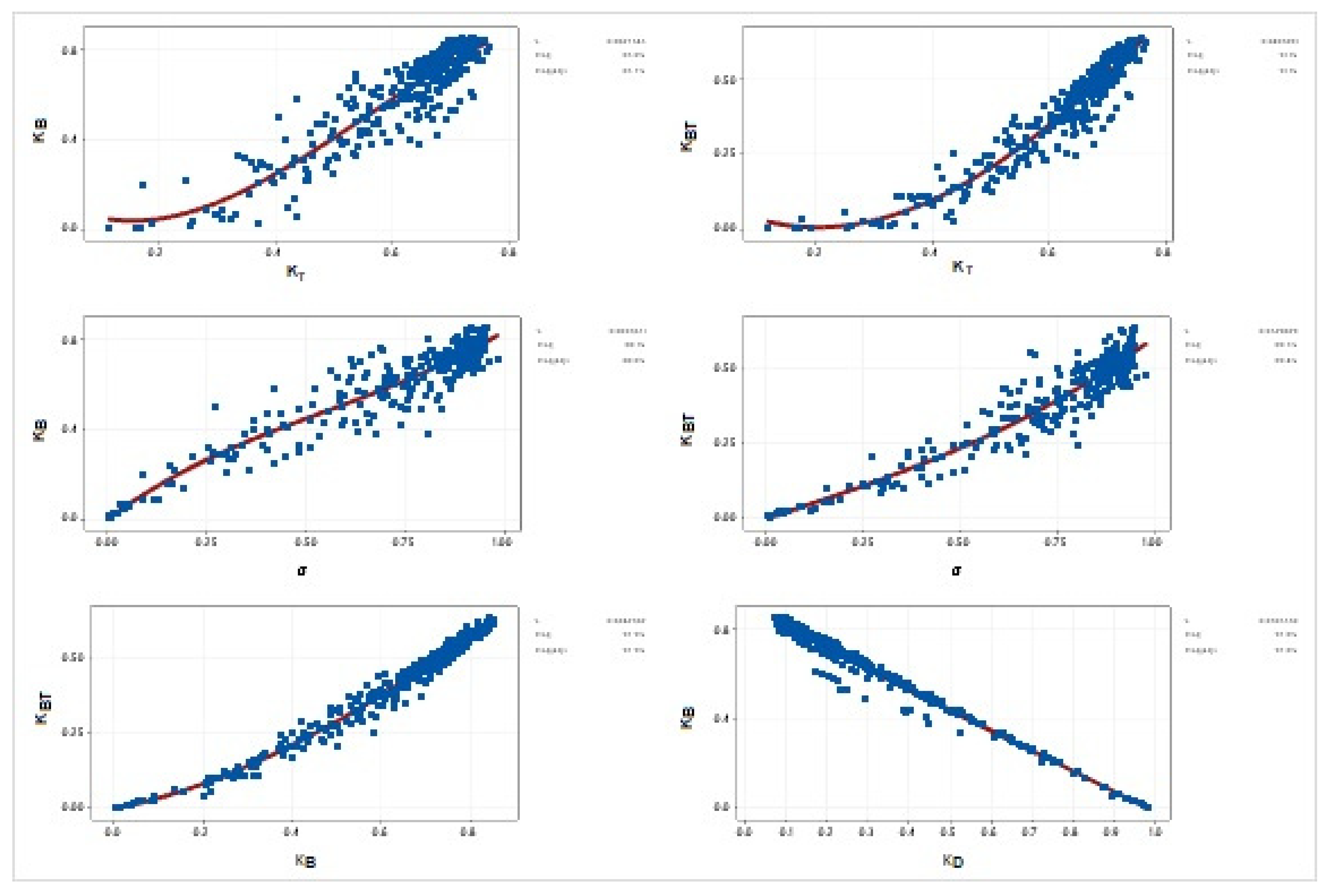
Figure 29.
Relationships between various daily radiation indices.
Figure 29.
Relationships between various daily radiation indices.
Table 1.
Station’s coordinates and mean annual air temperature (Ta), mean annual precipitation (Prec) and mean annual number of hours of sunshine duration.
Table 1.
Station’s coordinates and mean annual air temperature (Ta), mean annual precipitation (Prec) and mean annual number of hours of sunshine duration.
| Station | Long. (E)
(deg.) | Lat. (N)
(deg.) | Elev. (m) | Distance from Coast (km) | Ta (°C) | Prec. (mm) | Sunshine Duration (hrs) |
|---|
| Athalassa | 33.396 | 35.141 | 158 | 20 | 19.8 | 315 | 3285 |
Table 2.
Solar Shortwave Radiation equipment installed at the actinometric station of Athalassa.
Table 2.
Solar Shortwave Radiation equipment installed at the actinometric station of Athalassa.
| Parameter | Symbol | Unit | Type | Model | Manufacturer | Spectral Range | Calibration Factor | Max Output | Note |
|---|
| Global Horizontal Irradiance | Gt | W m−2 | Pyranometer | CM6B | Kipp&Zonen | 305–2800 nm | 12.93 μV/(W m−2) | 1500 W m−2 | On 2AP Suntracker |
| Direct Normal Irradiance | Bn | W m−2 | Pyrheliometer | CH1 | Kipp&Zonen | 350–1500 nm | 11.03 μV/(W m−2) | 1500 W m−2 | On 2AP Suntracker |
| Direct Horizontal Irradiance | B | W m−2 | Pyrheliometer | CH1 | Kipp&Zonen | 350–1500 nm | 11.03 μV/(W m−2) | 1500 W m−2 | B = Bn *cos θz (θz = Solar Zen. Angle) |
| Sunshine Duration | S | W m−2 | Pyrheliometer | CH1 | Kipp&Zonen | 350–1500 nm | 11.03 μV/(W m−2) | 1500 W m−2 | Time in min when Bn > 120 W/m2 |
| Diffuse Horizontal Irradiance | D | W m−2 | Pyranometer | CM6B | Kipp&Zonen | 305–2800 nm | 9.88 μV/(W m−2) | 1500 W m−2 | On 2AP with shading ball arm |
| Reflected Horizontal Irradiance | R | W m−2 | Pyranometer | CM11 | Kipp&Zonen | 310–2800 nm | 5.12 μV/(W m−2) | 1500 W m−2 | Albedometer |
| Photosynthetic Photon Flux Dens. | GPPFD | μmol s−1m−2 | Quantum Sens. | Li190SA | Light Comp. | 400–700 nm | 347.087 μmol s−1m−2mV−1 | 2500 μmol s−1m−2 | 4.57 μmol s−1m−2 PPFD = 1 Wm−2 PAR |
| Diffuse PPFD | DPPFD | μmol s−1m−2 | Quantum Sens. | Li190SA | Light Comp. | 400–700 nm | 4.96 μmol s−1m−2μV−1 | 2500 μmol s−1m−2 | On 2AP with shading ball arm |
Table 3.
BSRN-Physically Possible Limits (PPL), Extremely Rare Limits (ERL), and Configurable Climatological Limits (CCL) [
27].
Ldn and
Lup are the downward and upward longwave irradiances.
Table 3.
BSRN-Physically Possible Limits (PPL), Extremely Rare Limits (ERL), and Configurable Climatological Limits (CCL) [
27].
Ldn and
Lup are the downward and upward longwave irradiances.
| | Lower Bound (W/m2) | Upper Bound (W/m2) | Upper Bound (W/m2) |
|---|
| Parameter | PPL | ERL | PPL | ERL | CCL | Level |
|---|
| G | −4 | −2 | min(1.2*G0n, 1.5*G0n*(cosθz)1.2 + 100) | 1.2*G0n*(cosθz)1.2 + 50 | 0.97*G0n*(cosθz)1.2 + 55 | 2nd |
| | | | | | 0.92*G0n*(cosθz)1.2 + 50 | 1st |
| D | −4 | −2 | min(0.8*G0n , 0.95*G0n*(cosθz)1.2 + 50) | 0.75*G0n*(cosθz)1.2 + 30 | 0.58*G0n*(cosθz)1.2 + 35 | 2nd |
| | | | | | 0.52*G0n*(cosθz)1.2 + 30 | 1st |
| Bn | −4 | −2 | G0n | 0.95*G0n*(cosθz)0.2 + 10 | 0.86*G0n*(cosθz)0.2 + 15 | 2nd |
| | | | | | 0.82*G0n*(cosθz)0.2 + 10 | 1st |
| B | −4 | −2 | G0n*(cosθz) | 0.95*G0n*(cosθz)1.2 + 10 | 0.86*G0n*(cosθz)1.2 + 15 | 2nd |
| | | | | | 0.82*G0n*(cosθz)1.2 + 10 | 1st |
| R | −4 | −4 | 1.2*G0n*(cosθz)1.2 + 50 | G0n*(cosθz)1.2 + 50 | 0.95*G0n*(cosθz)1.2 + 55 | 2nd |
| | | | | | 0.87*G0n*(cosθz)1.2 + 50 | 1st |
| Ldn | 40 | 60 | 700 | 500 | LL: 145 UL: 500 | 2nd |
| | | | | | LL: 190 UL: 465 | 1st |
| Lup | 40 | 60 | 900 | 700 | LL: 210 UL: 630 | 2nd |
| | | | | | LL: 240 UL: 590 | 1st |
Table 4.
Daily Upper limits of Physically Possible tests (PPL) and Extremely Rare tests (ERL) (Lower limit of
Gd is 0.03 ×
G0d) [
5].
Table 4.
Daily Upper limits of Physically Possible tests (PPL) and Extremely Rare tests (ERL) (Lower limit of
Gd is 0.03 ×
G0d) [
5].
| Parameter | PPL
ERL | Upper Limit (MJ/m2) |
|---|
| Global irradiation (Gd) vs. G0d | PPL | Gd < G0d |
| Global irradiation (Gd) vs. G0d | ERL | Gd < 0.8 × G0d |
| Global irradiation (Gd) vs. Gcd | ERL | Gd < 1.1 × Gcd |
| Diffuse irradiation (Dd) vs. G0d | PPL | Dd < 1.0 × G0d |
| Diffuse irradiation (Dd) vs. G0d | ERL | Dd < 0.7 × G0d |
| Beam Normal irrad. (Bnd) vs. G0nd | PPL | Bnd < 1.0 × G0nd |
| Beam Normal irrad. (Bnd) vs. G0nd | ERL | Bnd < 0.8 × G0nd |
| Beam Horizontal irrad. (Bd) vs. G0d | PPL | Bd < 1.0 × G0d |
| Beam Horizontal irrad. (Bd) vs. G0d | ERL | Bd < 0.8 × G0d |
| Beam Horizontal irrad. (Bd) vs. Bcd | PPL | Bd < 1.1 × Bcd |
| Consistency test [Sum Bd + Dd)/Gd] | PPL | Range of 0.9 to 1.1 |
| Daily Sunshine Duration (Sd) vs. S0d | PRL | Sd < S0d |
Table 5.
Monthly descriptive statistics of the shortwave solar radiation components (W/m2).
Table 5.
Monthly descriptive statistics of the shortwave solar radiation components (W/m2).
| | Bn [W/m2] | | | | | | | | B [W/m2] | | | | | | | |
|---|
| Month | N | Mean | StDev | Min | Q1 | Median | Q3 | Max | N | Mean | StDev | Min | Q1 | Median | Q3 | Max |
|---|
| 1 | 1841 | 298 | 312 | 0 | 2 | 175 | 584 | 940 | 1841 | 130 | 156 | 0 | 1 | 53 | 235 | 546 |
| 2 | 1796 | 467 | 331 | 0 | 87 | 547 | 771 | 960 | 1796 | 236 | 208 | 0 | 22 | 201 | 421 | 671 |
| 3 | 2187 | 382 | 315 | 0 | 26 | 399 | 655 | 946 | 2187 | 225 | 220 | 0 | 6 | 167 | 399 | 744 |
| 4 | 2318 | 424 | 315 | 0 | 76 | 461 | 716 | 945 | 2318 | 287 | 265 | 0 | 22 | 234 | 507 | 866 |
| 5 | 2576 | 552 | 262 | 0 | 396 | 638 | 765 | 869 | 2576 | 389 | 267 | 0 | 133 | 399 | 632 | 832 |
| 6 | 2548 | 571 | 280 | 0 | 399 | 671 | 790 | 930 | 2548 | 407 | 289 | 0 | 122 | 412 | 678 | 905 |
| 7 | 2627 | 611 | 250 | 0 | 487 | 708 | 799 | 917 | 2627 | 434 | 280 | 0 | 168 | 461 | 704 | 890 |
| 8 | 2473 | 615 | 247 | 0 | 509 | 701 | 798 | 907 | 2473 | 418 | 266 | 0 | 166 | 447 | 665 | 845 |
| 9 | 2197 | 526 | 232 | 0 | 395 | 614 | 707 | 834 | 2197 | 332 | 218 | 0 | 122 | 353 | 535 | 679 |
| 10 | 2052 | 503 | 283 | 0 | 281 | 599 | 730 | 899 | 2052 | 274 | 204 | 0 | 75 | 268 | 457 | 697 |
| 11 | 1821 | 293 | 300 | 0 | 0 | 175 | 603 | 874 | 1821 | 134 | 156 | 0 | 0 | 53 | 263 | 519 |
| 12 | 1800 | 343 | 323 | 0 | 2 | 276 | 667 | 896 | 1800 | 143 | 153 | 0 | 0 | 76 | 289 | 473 |
| Year | 26,236 | 478 | 307 | 0 | 169 | 574 | 743 | 960 | 26,236 | 298 | 258 | 0 | 40 | 261 | 507 | 905 |
| | D [W/m2] | | | | | | | | G [W/m2] | | | | | | | |
| Month | N | Mean | StDev | Min | Q1 | Median | Q3 | Max | N | Mean | StDev | Min | Q1 | Median | Q3 | Max |
| 1 | 1600 | 138 | 80 | 0 | 75 | 114 | 193 | 403 | 1600 | 311 | 177 | 7 | 156 | 287 | 461 | 737 |
| 2 | 1594 | 125 | 77 | 0 | 68 | 104 | 160 | 444 | 1594 | 428 | 223 | 14 | 228 | 439 | 630 | 907 |
| 3 | 1969 | 166 | 111 | 1 | 77 | 130 | 231 | 556 | 1970 | 476 | 262 | 7 | 245 | 464 | 717 | 1119 |
| 4 | 2112 | 168 | 111 | 6 | 88 | 134 | 220 | 586 | 2112 | 549 | 299 | 12 | 277 | 553 | 831 | 1146 |
| 5 | 2346 | 119 | 80 | 12 | 64 | 88 | 153 | 474 | 2346 | 632 | 299 | 34 | 372 | 686 | 915 | 1145 |
| 6 | 2335 | 117 | 73 | 13 | 66 | 90 | 158 | 585 | 1080 | 635 | 298 | 46 | 379 | 679 | 918 | 1142 |
| 7 | 2393 | 92 | 47 | 10 | 64 | 85 | 108 | 408 | 2393 | 628 | 293 | 45 | 373 | 681 | 907 | 1107 |
| 8 | 2254 | 89 | 45 | 5 | 59 | 80 | 105 | 304 | 2254 | 613 | 284 | 54 | 366 | 666 | 877 | 1126 |
| 9 | 1990 | 108 | 46 | 14 | 83 | 103 | 129 | 389 | 1990 | 553 | 250 | 54 | 340 | 600 | 786 | 907 |
| 10 | 1832 | 111 | 61 | 14 | 68 | 96 | 136 | 428 | 1832 | 467 | 215 | 37 | 286 | 489 | 657 | 891 |
| 11 | 1593 | 131 | 77 | 3 | 73 | 111 | 175 | 438 | 1593 | 312 | 186 | 12 | 146 | 290 | 478 | 785 |
| 12 | 1550 | 106 | 64 | 0 | 61 | 85 | 144 | 341 | 1550 | 296 | 170 | 7 | 141 | 279 | 458 | 719 |
| Year | 23,568 | 122 | 79 | 0 | 68 | 98 | 150 | 586 | 22,314 | 504 | 283 | 7 | 254 | 494 | 743 | 1146 |
Table 6.
Statistical values of all radiation components considering the prevailing weather conditions as classified by the clearness index (kt).
Table 6.
Statistical values of all radiation components considering the prevailing weather conditions as classified by the clearness index (kt).
| | | kt ≤ 0.35 (Cloudy) | kt > 0.65 (Clear Sky) |
|---|
| Var. | Unit | Fraction of G (%) | Mean | Median | Min | Max | Std. Dev. | Fraction of G (%) | Mean | Median | Min | Max | Std. Dev. |
|---|
| G | W/m2 | | 135.9 | 118 | 7 | 446.0 | 82.69 | | 668.7 | 675 | 110 | 1146.0 | 210.27 |
| UVB | W/m2 | 0.12 | 0.2 | 0 | 0 | 1.3 | 0.18 | 0.14 | 0.9 | 1 | 0 | 2.2 | 0.53 |
| UVA | W/m2 | 6.63 | 9.0 | 8 | 0 | 35.0 | 5.70 | 5.20 | 34.8 | 34 | 3 | 61.5 | 13.08 |
| UVE | W/m2 | 0.01 | 0.0 | 0 | 0 | 0.1 | 0.02 | 0.01 | 0.1 | 0 | 0 | 0.2 | 0.06 |
| UVT | W/m2 | 6.75 | 9.2 | 8 | 0 | 35.9 | 5.90 | 5.34 | 35.7 | 35 | 3 | 63.6 | 13.60 |
| Bn | W/m2 | 9.82 | 13.4 | 0 | 0 | 584.0 | 38.49 | 105.36 | 704.6 | 722 | 1 | 960.0 | 127.44 |
| B | W/m2 | 4.08 | 5.6 | 0 | 0 | 201.0 | 16.15 | 71.20 | 476.2 | 467 | 0 | 890.2 | 186.26 |
| D | W/m2 | 84.91 | 115.4 | 102 | 1 | 406.0 | 74.39 | 17.59 | 117.6 | 99 | 26 | 578.0 | 65.87 |
| RF | W/m2 | 9.25 | 12.6 | 8 | 0 | 69.0 | 13.73 | 18.92 | 126.5 | 129 | 1 | 238.0 | 44.05 |
| GPPFD | μmol/s/m2 | | 232.7 | 200 | 24 | 897.0 | 140.67 | | 1150.5 | 1154 | 118 | 2113.0 | 413.32 |
| GPAR | W/m2 | 37.46 | 50.9 | 44 | 5 | 196.3 | 30.78 | 37.65 | 251.8 | 253 | 26 | 462.4 | 90.44 |
| DPPFD | μmol/s/m2 | | 269.7 | 238 | 2 | 958.0 | 164.95 | | 324.9 | 291 | 89 | 1297.0 | 141.89 |
| DPAR | W/m2 | 43.42 | 59.0 | 52 | 0 | 209.6 | 36.10 | 10.63 | 71.1 | 64 | 19 | 283.8 | 31.05 |
| NIR | W/m2 | 55.79 | 75.8 | 66 | 0 | 248.1 | 48.39 | 57.02 | 381.3 | 384 | 66 | 750.8 | 114.22 |
| Lupd | W/m2 | 293.58 | 399.1 | 390 | 315 | 626.0 | 42.12 | 78.78 | 526.8 | 534 | 318 | 704.0 | 88.78 |
| Ldnd | W/m2 | 253.77 | 345.0 | 348 | 244 | 452.0 | 29.10 | 52.34 | 350.1 | 355 | 235 | 461.0 | 40.56 |
| | | 0.35 < kt ≤ 0.55 (Partially Cloudy ) | 0.55 < kt ≤ 0.65 (Partially Cloudy ) |
| Var. | Unit | Fraction of G (%) | Mean | Median | Min | Max | Std. Dev. | Fraction of G (%) | Mean | Median | Min | Max | Std. Dev. |
| G | W/m2 | | 235.1 | 199 | 58 | 700.0 | 133.14 | | 304.6 | 276 | 94 | 817.0 | 139.62 |
| UVB | W/m2 | 0.10 | 0.2 | 0 | 0 | 1.6 | 0.25 | 0.08 | 0.3 | 0 | 0 | 1.8 | 0.25 |
| UVA | W/m2 | 5.43 | 12.8 | 10 | 2 | 43.1 | 8.25 | 4.79 | 14.6 | 13 | 4 | 50.8 | 8.15 |
| UVE | W/m2 | 0.01 | 0.0 | 0 | 0 | 0.2 | 0.03 | 0.01 | 0.0 | 0 | 0 | 0.2 | 0.03 |
| UVT | W/m2 | 5.53 | 13.0 | 10 | 2 | 44.7 | 8.49 | 4.88 | 14.9 | 13 | 4 | 52.6 | 8.40 |
| Bn | W/m2 | 77.75 | 182.8 | 164 | 0 | 691.0 | 142.27 | 140.24 | 427.1 | 446 | 0 | 782.0 | 131.46 |
| B | W/m2 | 25.06 | 58.9 | 45 | 0 | 384.9 | 54.30 | 50.73 | 154.5 | 146 | 0 | 568.5 | 76.55 |
| D | W/m2 | 64.21 | 151.0 | 118 | 5 | 586.0 | 114.64 | 37.34 | 113.7 | 81 | 16 | 556.0 | 90.69 |
| RF | W/m2 | 14.10 | 33.1 | 28 | 0 | 127.0 | 24.96 | 16.42 | 50.0 | 47 | 0 | 162.0 | 29.50 |
| GPPFD | μmol/s/m2 | | 395.7 | 347 | 86 | 1335.0 | 214.53 | | 513.1 | 471 | 78 | 1574.0 | 242.81 |
| GPAR | W/m2 | 36.84 | 86.6 | 76 | 19 | 292.1 | 46.94 | 36.86 | 112.3 | 103 | 17 | 344.4 | 53.13 |
| DPPFD | μmol/s/m2 | | 356.0 | 279 | 56 | 1298.0 | 241.85 | | 294.3 | 231 | 76 | 1227.0 | 190.19 |
| DPAR | W/m2 | 33.13 | 77.9 | 61 | 12 | 284.0 | 52.92 | 21.14 | 64.4 | 51 | 17 | 268.5 | 41.62 |
| NIR | W/m2 | 57.64 | 135.5 | 114 | 23 | 404.0 | 80.89 | 58.26 | 177.4 | 158 | 52 | 483.9 | 82.41 |
| Lupd | W/m2 | 184.95 | 434.8 | 424 | 319 | 659.0 | 53.41 | 146.94 | 447.5 | 432 | 314 | 665.0 | 63.17 |
| Ldnd | W/m2 | 144.47 | 339.6 | 342 | 235 | 453.0 | 32.61 | 110.01 | 335.1 | 335 | 235 | 438.0 | 37.00 |
Table 7.
Monthly statistics of direct normal (Bn), direct horizontal (B), diffuse (D) and global irradiance (G) in (W/m2) for cloudy, partially cloudy and clear sky conditions.
Table 7.
Monthly statistics of direct normal (Bn), direct horizontal (B), diffuse (D) and global irradiance (G) in (W/m2) for cloudy, partially cloudy and clear sky conditions.
| | Cloudy (kt ≤ 0.35) |
|---|
| | Bn | B | D | G |
|---|
| Month | Mean | StDev | Median | Max | Mean | StDev | Median | Max | Mean | StDev | Median | Max | Mean | StDev | Median | Max |
|---|
| 1 | 10.9 | 28.0 | 0.0 | 213 | 3.7 | 10.6 | 0.0 | 104 | 112.0 | 61.5 | 104.0 | 274 | 118.8 | 64.2 | 112.0 | 277 |
| 2 | 10.7 | 26.6 | 0.0 | 170 | 4.3 | 12.7 | 0.0 | 115 | 126.7 | 70.7 | 116.0 | 325 | 134.3 | 74.5 | 129.0 | 328 |
| 3 | 9.0 | 22.6 | 0.0 | 141 | 4.5 | 11.9 | 0.0 | 90 | 139.6 | 90.5 | 119.0 | 368 | 148.7 | 95.7 | 126.0 | 384 |
| 4 | 9.2 | 24.8 | 0.0 | 161 | 3.9 | 12.6 | 0.0 | 122 | 142.8 | 99.5 | 116.0 | 403 | 151.6 | 104.8 | 120.0 | 427 |
| 5 | 36.7 | 46.1 | 15.5 | 206 | 18.2 | 25.5 | 6.5 | 90 | 126.7 | 89.7 | 97.0 | 365 | 156.9 | 111.3 | 124.5 | 428 |
| 6 | 24.4 | 43.2 | 1.0 | 218 | 13.6 | 28.2 | 0.7 | 166 | 159.2 | 89.7 | 163.0 | 406 | 180.4 | 107.4 | 176.0 | 444 |
| 7 | 114.2 | 103.2 | 111.0 | 317 | 29.8 | 39.4 | 23.9 | 201 | 85.0 | 82.1 | 40.5 | 319 | 122.8 | 104.7 | 67.5 | 396 |
| 8 | 133.8 | 103.4 | 134.0 | 339 | 36.2 | 32.7 | 31.1 | 155 | 89.1 | 77.8 | 51.5 | 297 | 134.6 | 96.5 | 82.0 | 367 |
| 9 | 74.1 | 73.3 | 51.5 | 251 | 20.2 | 24.1 | 15.5 | 118 | 97.7 | 86.1 | 55.5 | 301 | 128.2 | 99.9 | 71.5 | 366 |
| 10 | 44.7 | 58.5 | 24.0 | 248 | 17.7 | 28.9 | 6.6 | 177 | 108.5 | 69.9 | 94.0 | 326 | 134.3 | 85.7 | 110.0 | 342 |
| 11 | 13.7 | 33.3 | 0.0 | 198 | 4.8 | 12.4 | 0.0 | 91 | 107.1 | 68.2 | 90.0 | 276 | 115.5 | 72.0 | 96.0 | 290 |
| 12 | 14.1 | 31.5 | 0.0 | 211 | 4.6 | 11.3 | 0.0 | 109 | 95.7 | 58.0 | 89.0 | 233 | 103.8 | 62.7 | 99.0 | 260 |
| | Partly cloudy with predominance of the diffuse component (0.35 < kt ≤ 0.55) |
| | Bn | B | D | G |
| Month | Mean | StDev | Median | Max | Mean | StDev | Median | Max | Mean | StDev | Median | Max | Mean | StDev | Median | Max |
| 1 | 145.1 | 131.0 | 100.0 | 496 | 51.3 | 47.0 | 37.9 | 247 | 184.1 | 87.3 | 189.5 | 371 | 245.2 | 92.3 | 254.0 | 436 |
| 2 | 189.1 | 126.7 | 186.0 | 522 | 67.6 | 56.4 | 56.6 | 333 | 171.6 | 103.0 | 154.5 | 429 | 252.8 | 120.2 | 248.5 | 495 |
| 3 | 118.7 | 102.5 | 91.5 | 472 | 58.5 | 59.0 | 40.2 | 326 | 244.7 | 124.4 | 239.0 | 494 | 321.6 | 145.7 | 338.0 | 614 |
| 4 | 122.8 | 109.6 | 100.0 | 482 | 50.9 | 52.2 | 34.7 | 378 | 238.3 | 147.6 | 219.0 | 586 | 308.3 | 160.3 | 297.0 | 666 |
| 5 | 227.4 | 116.4 | 222.0 | 465 | 73.8 | 63.4 | 54.0 | 337 | 126.6 | 111.5 | 80.0 | 447 | 223.0 | 158.9 | 152.0 | 692 |
| 6 | 285.9 | 124.9 | 300.0 | 522 | 91.1 | 69.3 | 74.0 | 464 | 110.3 | 105.2 | 59.0 | 441 | 218.2 | 156.9 | 155.0 | 670 |
| 7 | 376.5 | 104.1 | 385.0 | 598 | 98.0 | 51.4 | 90.2 | 462 | 57.4 | 51.2 | 44.5 | 408 | 164.6 | 87.3 | 147.5 | 654 |
| 8 | 390.7 | 105.5 | 399.0 | 604 | 103.2 | 55.9 | 92.9 | 388 | 54.5 | 41.9 | 43.5 | 281 | 166.2 | 88.1 | 147.0 | 676 |
| 9 | 308.6 | 102.4 | 317.0 | 514 | 86.3 | 55.2 | 75.1 | 404 | 72.9 | 52.8 | 59.0 | 379 | 178.3 | 95.0 | 157.0 | 612 |
| 10 | 279.1 | 122.2 | 285.0 | 564 | 87.9 | 56.5 | 77.1 | 316 | 112.2 | 84.3 | 77.0 | 404 | 215.8 | 120.4 | 173.0 | 530 |
| 11 | 177.0 | 142.0 | 152.0 | 539 | 62.3 | 57.5 | 47.7 | 286 | 172.3 | 94.1 | 164.0 | 374 | 246.1 | 98.8 | 260.0 | 472 |
| 12 | 193.8 | 147.7 | 162.0 | 540 | 58.4 | 47.3 | 50.6 | 270 | 140.4 | 84.0 | 130.0 | 315 | 212.0 | 91.2 | 200.0 | 394 |
| | Partly cloudy with predominance of the direct component (0.55 < kt ≤ 0.65) |
| | Bn | B | D | G |
| Month | Mean | StDev | Median | Max | Mean | StDev | Median | Max | Mean | StDev | Median | Max | Mean | StDev | Median | Max |
| 1 | 441.8 | 130.5 | 462.5 | 687 | 168.0 | 70.6 | 162.8 | 333 | 144.0 | 79.8 | 130.5 | 383 | 330.6 | 112.5 | 344.5 | 525 |
| 2 | 436.3 | 129.6 | 454.5 | 688 | 147.5 | 77.5 | 129.0 | 426 | 123.5 | 88.0 | 90.5 | 444 | 293.2 | 133.8 | 256.0 | 589 |
| 3 | 336.8 | 126.5 | 337.0 | 656 | 148.6 | 79.9 | 130.1 | 404 | 206.3 | 138.8 | 180.0 | 515 | 392.3 | 185.8 | 389.5 | 745 |
| 4 | 349.7 | 127.1 | 342.0 | 639 | 150.8 | 89.4 | 127.3 | 532 | 180.8 | 133.5 | 146.0 | 556 | 373.2 | 198.1 | 312.0 | 800 |
| 5 | 447.0 | 99.4 | 457.5 | 654 | 175.7 | 84.6 | 160.8 | 587 | 116.0 | 94.6 | 77.5 | 420 | 328.2 | 163.8 | 286.5 | 787 |
| 6 | 502.3 | 93.7 | 519.0 | 691 | 198.6 | 89.6 | 178.5 | 599 | 96.3 | 73.4 | 67.0 | 379 | 322.1 | 152.0 | 277.0 | 796 |
| 7 | 552.2 | 74.7 | 565.0 | 686 | 236.9 | 68.4 | 230.1 | 457 | 86.3 | 55.0 | 71.0 | 396 | 348.3 | 109.9 | 330.0 | 801 |
| 8 | 564.5 | 70.1 | 569.0 | 722 | 240.7 | 83.6 | 228.8 | 577 | 81.4 | 42.3 | 72.0 | 303 | 345.9 | 121.5 | 328.5 | 780 |
| 9 | 500.5 | 74.9 | 509.0 | 659 | 217.1 | 79.2 | 208.0 | 460 | 101.1 | 49.1 | 92.0 | 389 | 354.6 | 117.2 | 340.5 | 727 |
| 10 | 515.5 | 98.7 | 530.0 | 718 | 199.8 | 78.7 | 189.4 | 440 | 101.5 | 55.0 | 86.0 | 315 | 323.9 | 110.4 | 307.0 | 625 |
| 11 | 478.8 | 120.4 | 501.0 | 692 | 179.6 | 67.9 | 180.9 | 376 | 121.9 | 73.8 | 99.0 | 438 | 321.7 | 105.8 | 308.0 | 562 |
| 12 | 505.0 | 137.7 | 549.0 | 691 | 163.6 | 57.7 | 165.9 | 321 | 97.5 | 61.7 | 72.0 | 322 | 280.7 | 79.9 | 271.0 | 467 |
| | Clear (kt > 0.65) |
| | Bn | B | D | G |
| Month | Mean | StDev | Median | Max | Mean | StDev | Median | Max | Mean | StDev | Median | Max | Mean | StDev | Median | Max |
| 1 | 719.1 | 142.5 | 738.5 | 940 | 344.0 | 109.2 | 351.6 | 546 | 119.0 | 71.6 | 94.0 | 403 | 489.9 | 114.9 | 511.5 | 715 |
| 2 | 743.5 | 131.9 | 760.5 | 960 | 403.2 | 139.6 | 409.3 | 671 | 114.4 | 62.8 | 98.5 | 440 | 549.5 | 151.6 | 583.5 | 880 |
| 3 | 660.4 | 158.8 | 657.0 | 946 | 407.1 | 164.9 | 401.2 | 744 | 146.9 | 95.8 | 118.0 | 556 | 625.4 | 191.8 | 668.0 | 1121 |
| 4 | 678.1 | 160.2 | 696.0 | 945 | 490.9 | 192.8 | 486.7 | 866 | 152.7 | 86.7 | 130.0 | 578 | 713.7 | 201.5 | 759.0 | 1109 |
| 5 | 711.3 | 107.6 | 723.0 | 869 | 546.6 | 179.5 | 564.3 | 832 | 118.3 | 69.9 | 90.0 | 474 | 739.2 | 198.6 | 782.0 | 1088 |
| 6 | 752.3 | 99.6 | 761.0 | 930 | 593.9 | 184.1 | 625.5 | 905 | 118.0 | 61.5 | 95.0 | 585 | 762.7 | 199.2 | 814.0 | 1139 |
| 7 | 765.5 | 75.9 | 781.0 | 917 | 614.7 | 163.5 | 652.4 | 890 | 99.6 | 37.7 | 94.0 | 370 | 762.9 | 174.4 | 808.5 | 1081 |
| 8 | 768.3 | 77.8 | 778.0 | 907 | 593.8 | 153.2 | 621.6 | 845 | 96.8 | 41.0 | 87.0 | 304 | 741.2 | 164.3 | 781.0 | 1078 |
| 9 | 686.6 | 68.0 | 696.0 | 834 | 495.7 | 115.5 | 515.7 | 679 | 119.5 | 33.3 | 116.0 | 388 | 680.2 | 125.7 | 712.0 | 865 |
| 10 | 723.1 | 103.8 | 727.0 | 899 | 442.7 | 119.9 | 454.0 | 697 | 114.6 | 53.6 | 102.0 | 428 | 587.9 | 118.9 | 611.0 | 854 |
| 11 | 675.9 | 111.6 | 688.0 | 874 | 343.8 | 89.3 | 355.6 | 519 | 132.2 | 61.3 | 115.0 | 402 | 502.9 | 99.6 | 517.0 | 765 |
| 12 | 720.4 | 102.1 | 745.0 | 896 | 336.7 | 74.1 | 347.2 | 473 | 102.9 | 54.6 | 80.0 | 341 | 462.2 | 76.8 | 480.0 | 701 |
Table 8.
Mean daily and extreme values and the standard deviations of the shortwave radiation components for each month of the year in MJ/m2. The last column shows the respective daily values of sunshine duration. Note: * means no records.
Table 8.
Mean daily and extreme values and the standard deviations of the shortwave radiation components for each month of the year in MJ/m2. The last column shows the respective daily values of sunshine duration. Note: * means no records.
| | Bnd (MJ/m2) | Bd (MJ/m2) | Dd (MJ/m2) | Gd (MJ/m2) | Sd (hrs) |
|---|
| Month | Mean | StDev | Min | Max | Mean | StDev | Min | Max | Mean | StDev | Min | Max | Mean | StDev | Min | Max | Mean | StDev | Min | Max |
|---|
| 1 | 10.6 | 7.2 | 0.6 | 24.7 | 4.6 | 3.2 | 0.2 | 10.4 | 4.3 | 1.4 | 1.9 | 6.8 | 9.5 | 2.7 | 3.2 | 14.0 | 5.1 | 2.6 | 0.3 | 9.1 |
| 2 | 18.0 | 8.1 | 0.0 | 30.2 | 9.1 | 4.2 | 0.0 | 15.6 | 4.3 | 1.6 | 1.6 | 7.3 | 14.3 | 3.5 | 3.9 | 18.4 | 7.6 | 2.6 | 0.0 | 10.1 |
| 3 | 16.2 | 8.5 | 0.5 | 31.2 | 9.5 | 5.0 | 0.3 | 17.8 | 6.3 | 2.3 | 2.1 | 10.1 | 17.8 | 4.2 | 7.6 | 23.8 | * | * | * | * |
| 4 | 19.7 | 10.0 | 1.4 | 35.9 | 13.3 | 6.8 | 0.8 | 23.6 | 7.1 | 2.9 | 2.3 | 13.4 | 22.6 | 5.0 | 12.2 | 27.9 | 9.0 | 3.6 | 0.7 | 12.5 |
| 5 | 27.5 | 5.7 | 13.2 | 34.4 | 19.4 | 3.7 | 9.7 | 23.8 | 5.4 | 2.6 | 2.5 | 11.4 | 27.7 | 1.7 | 22.6 | 29.8 | 12.0 | 1.4 | 8.9 | 14.0 |
| 6 | 29.3 | 5.9 | 14.7 | 37.4 | 20.8 | 4.1 | 9.4 | 26.1 | 5.5 | 2.2 | 2.7 | 11.8 | 28.3 | 2.7 | 21.1 | 30.9 | 12.5 | 1.7 | 8.3 | 13.6 |
| 7 | 31.1 | 2.5 | 25.8 | 35.6 | 22.0 | 1.5 | 18.5 | 25.1 | 4.3 | 1.2 | 2.4 | 7.9 | 28.1 | 0.8 | 26.3 | 30.4 | 12.8 | 0.6 | 11.3 | 13.6 |
| 8 | 29.4 | 3.4 | 21.1 | 35.2 | 20.0 | 2.3 | 14.4 | 23.9 | 3.9 | 1.2 | 2.0 | 6.5 | 25.7 | 1.5 | 21.9 | 27.9 | 12.2 | 0.5 | 10.9 | 12.9 |
| 9 | 23.1 | 3.0 | 13.4 | 27.0 | 14.5 | 2.0 | 8.5 | 17.2 | 4.3 | 1.1 | 2.8 | 8.4 | 21.0 | 1.4 | 17.4 | 23.0 | 10.8 | 0.9 | 8.2 | 11.8 |
| 10 | 20.1 | 5.4 | 7.6 | 28.3 | 10.9 | 3.2 | 3.7 | 16.1 | 4.0 | 1.4 | 2.0 | 7.3 | 15.9 | 2.2 | 11.8 | 19.6 | 9.0 | 1.4 | 5.5 | 10.4 |
| 11 | 10.7 | 6.6 | 0.1 | 22.0 | 4.9 | 3.1 | 0.0 | 9.4 | 4.2 | 1.0 | 2.0 | 5.9 | 9.6 | 2.8 | 2.9 | 13.4 | 5.1 | 2.9 | 0.0 | 8.9 |
| 12 | 11.9 | 7.1 | 0.0 | 22.2 | 5.0 | 2.9 | 0.0 | 8.9 | 3.2 | 1.2 | 1.6 | 5.4 | 8.7 | 2.5 | 1.9 | 11.2 | 5.5 | 2.6 | 0.1 | 8.5 |
| Year | 20.6 | 9.6 | 0.0 | 37.4 | 12.9 | 7.3 | 0.0 | 26.1 | 4.7 | 2.1 | 1.6 | 13.4 | 19.1 | 7.8 | 1.9 | 30.9 | 9.2 | 3.6 | 0.0 | 14.0 |
Table 9.
Monthly statistics of KT and the number of days (N) and their percentage according to the classification of days with respect to KT for each month of the year.
Table 9.
Monthly statistics of KT and the number of days (N) and their percentage according to the classification of days with respect to KT for each month of the year.
| | KT | I | II | III | IV |
|---|
| Month | Mean | StDev | CV(%) | Min | Q1 | Median | Q3 | Max | N | Perc(%) | N | Perc(%) | N | Perc(%) | N | Perc(%) |
|---|
| 1 | 0.519 | 0.137 | 26.460 | 0.177 | 0.432 | 0.493 | 0.629 | 0.715 | 4 | 12.90 | 13 | 41.94 | 8 | 25.81 | 6 | 19.35 |
| 2 | 0.619 | 0.130 | 20.970 | 0.170 | 0.550 | 0.666 | 0.714 | 0.744 | 1 | 3.57 | 6 | 21.43 | 5 | 17.86 | 16 | 57.14 |
| 3 | 0.603 | 0.132 | 21.930 | 0.261 | 0.532 | 0.628 | 0.716 | 0.764 | 2 | 6.45 | 8 | 25.81 | 9 | 29.03 | 12 | 38.71 |
| 4 | 0.630 | 0.129 | 20.430 | 0.347 | 0.558 | 0.678 | 0.722 | 0.761 | 1 | 3.33 | 5 | 16.67 | 5 | 16.67 | 19 | 63.33 |
| 5 | 0.694 | 0.036 | 5.130 | 0.585 | 0.667 | 0.707 | 0.724 | 0.735 | 0 | | 0 | | 3 | 9.68 | 28 | 90.32 |
| 6 | 0.681 | 0.064 | 9.360 | 0.510 | 0.680 | 0.703 | 0.718 | 0.744 | 0 | | 4 | 13.33 | 1 | 3.33 | 25 | 83.33 |
| 7 | 0.692 | 0.019 | 2.770 | 0.643 | 0.679 | 0.698 | 0.704 | 0.733 | 0 | | 0 | | 1 | 3.23 | 30 | 96.77 |
| 8 | 0.688 | 0.027 | 3.890 | 0.614 | 0.677 | 0.692 | 0.706 | 0.737 | 0 | | 0 | | 3 | 9.68 | 28 | 90.32 |
| 9 | 0.662 | 0.027 | 4.080 | 0.566 | 0.659 | 0.667 | 0.679 | 0.699 | 0 | | 0 | | 5 | 16.67 | 25 | 83.33 |
| 10 | 0.634 | 0.052 | 8.210 | 0.507 | 0.598 | 0.646 | 0.680 | 0.698 | 0 | | 2 | 6.45 | 15 | 48.39 | 14 | 45.16 |
| 11 | 0.497 | 0.138 | 27.700 | 0.163 | 0.373 | 0.530 | 0.626 | 0.671 | 4 | 13.33 | 12 | 40.00 | 13 | 43.33 | 1 | 3.33 |
| 12 | 0.520 | 0.151 | 29.010 | 0.115 | 0.466 | 0.549 | 0.646 | 0.677 | 5 | 16.13 | 11 | 35.48 | 8 | 25.81 | 7 | 22.58 |
| Year | 0.620 | 0.121 | 19.440 | 0.115 | 0.577 | 0.664 | 0.700 | 0.763 | 17 | 4.66 | 61 | 16.71 | 76 | 20.82 | 211 | 57.81 |
Table 10.
Descriptive statistics of daily sunshine duration and its relative sunshine duration for each month of the year. Note: * means no records.
Table 10.
Descriptive statistics of daily sunshine duration and its relative sunshine duration for each month of the year. Note: * means no records.
| | Daily Sunshine Duration (Sd, hrs) | Relative Sunshine Duration (σ = Sd/S0d) |
|---|
| Month | N | Mean | StDev | CV(%) | Min | Q1 | Median | Q3 | Max | Mean | StDev | CV(%) | Min | Q1 | Median | Q3 | Max |
|---|
| 1 | 31 | 5.1 | 2.6 | 51.2 | 0.3 | 3.4 | 4.7 | 7.5 | 9.1 | 0.510 | 0.260 | 51.020 | 0.025 | 0.341 | 0.484 | 0.754 | 0.907 |
| 2 | 28 | 7.6 | 2.6 | 34.6 | 0.0 | 6.3 | 8.6 | 9.7 | 10.1 | 0.708 | 0.240 | 33.900 | 0.002 | 0.605 | 0.784 | 0.903 | 0.937 |
| 3 | | * | * | * | * | * | * | * | * | * | * | * | * | * | * | * | * |
| 4 | 29 | 9.0 | 3.6 | 40.6 | 0.7 | 7.4 | 10.1 | 11.7 | 12.5 | 0.691 | 0.276 | 39.930 | 0.055 | 0.583 | 0.805 | 0.897 | 0.949 |
| 5 | 31 | 12.0 | 1.4 | 11.2 | 8.9 | 10.8 | 12.4 | 13.1 | 14.0 | 0.868 | 0.091 | 10.440 | 0.657 | 0.805 | 0.901 | 0.939 | 0.984 |
| 6 | 19 | 12.5 | 1.7 | 13.6 | 8.3 | 12.4 | 13.2 | 13.5 | 13.6 | 0.868 | 0.118 | 13.620 | 0.577 | 0.866 | 0.916 | 0.941 | 0.946 |
| 7 | 31 | 12.8 | 0.6 | 4.6 | 11.3 | 12.6 | 13.0 | 13.2 | 13.6 | 0.912 | 0.043 | 4.720 | 0.791 | 0.896 | 0.933 | 0.940 | 0.947 |
| 8 | 31 | 12.2 | 0.5 | 4.4 | 10.9 | 12.0 | 12.2 | 12.6 | 12.9 | 0.920 | 0.039 | 4.240 | 0.805 | 0.920 | 0.935 | 0.946 | 0.953 |
| 9 | 30 | 10.8 | 0.9 | 8.4 | 8.2 | 10.4 | 11.1 | 11.5 | 11.8 | 0.892 | 0.068 | 7.670 | 0.672 | 0.885 | 0.917 | 0.932 | 0.949 |
| 10 | 31 | 9.0 | 1.4 | 15.9 | 5.5 | 8.4 | 9.6 | 10.0 | 10.4 | 0.815 | 0.123 | 15.090 | 0.508 | 0.767 | 0.850 | 0.905 | 0.940 |
| 11 | 30 | 5.1 | 2.9 | 56.6 | 0.0 | 3.0 | 6.1 | 7.4 | 8.9 | 0.501 | 0.284 | 56.640 | 0.002 | 0.289 | 0.588 | 0.730 | 0.898 |
| 12 | 30 | 5.5 | 2.6 | 47.6 | 0.1 | 3.5 | 5.9 | 8.1 | 8.5 | 0.572 | 0.272 | 47.600 | 0.013 | 0.363 | 0.614 | 0.837 | 0.878 |
| Year | 321 | 9.2 | 3.6 | 39.4 | 0.0 | 7.1 | 10.0 | 12.2 | 14.0 | 0.748 | 0.246 | 32.830 | 0.002 | 0.661 | 0.856 | 0.924 | 0.984 |
Table 11.
Descriptive statistics of the daily fraction of diffuse to global radiation (KD).
Table 11.
Descriptive statistics of the daily fraction of diffuse to global radiation (KD).
| Month | N | Mean | StDev | CV(%) | Min | Q1 | Median | Q3 | Max |
|---|
| 1 | 31 | 0.514 | 0.239 | 46.45 | 0.142 | 0.277 | 0.529 | 0.683 | 0.951 |
| 2 | 28 | 0.351 | 0.219 | 62.32 | 0.09 | 0.189 | 0.280 | 0.486 | 0.982 |
| 3 | 31 | 0.406 | 0.234 | 57.62 | 0.096 | 0.197 | 0.392 | 0.551 | 0.936 |
| 4 | 30 | 0.356 | 0.219 | 61.59 | 0.081 | 0.180 | 0.280 | 0.448 | 0.898 |
| 5 | 31 | 0.203 | 0.110 | 54.26 | 0.083 | 0.112 | 0.186 | 0.273 | 0.503 |
| 6 | 30 | 0.201 | 0.099 | 49.26 | 0.087 | 0.125 | 0.186 | 0.246 | 0.522 |
| 7 | 31 | 0.152 | 0.045 | 29.66 | 0.078 | 0.118 | 0.140 | 0.185 | 0.285 |
| 8 | 31 | 0.152 | 0.052 | 34.16 | 0.073 | 0.112 | 0.142 | 0.188 | 0.269 |
| 9 | 30 | 0.209 | 0.063 | 30.26 | 0.126 | 0.174 | 0.203 | 0.219 | 0.456 |
| 10 | 31 | 0.263 | 0.123 | 46.64 | 0.112 | 0.155 | 0.231 | 0.333 | 0.609 |
| 11 | 30 | 0.498 | 0.245 | 49.22 | 0.163 | 0.303 | 0.376 | 0.661 | 0.971 |
| 12 | 31 | 0.440 | 0.258 | 58.57 | 0.143 | 0.229 | 0.351 | 0.579 | 0.970 |
| Year | 365 | 0.312 | 0.216 | 69.39 | 0.073 | 0.154 | 0.229 | 0.392 | 0.982 |
Table 12.
Descriptive statistics of the daily fraction of direct to global radiation (KB) and daily direct transmittance (KBT).
Table 12.
Descriptive statistics of the daily fraction of direct to global radiation (KB) and daily direct transmittance (KBT).
| | | KB | KBT |
|---|
| Month | N | Mean | StDev | CV(%) | Min | Q1 | Median | Q3 | Max | Mean | StDev | CV(%) | Min | Q1 | Median | Q3 | Max |
|---|
| 1 | 31 | 0.434 | 0.226 | 52.03 | 0.029 | 0.276 | 0.423 | 0.657 | 0.784 | 0.252 | 0.172 | 68.26 | 0.011 | 0.109 | 0.202 | 0.406 | 0.561 |
| 2 | 28 | 0.59 | 0.208 | 35.20 | 0.003 | 0.455 | 0.657 | 0.742 | 0.849 | 0.39 | 0.171 | 43.86 | 0.001 | 0.241 | 0.437 | 0.520 | 0.627 |
| 3 | 31 | 0.495 | 0.208 | 42.04 | 0.038 | 0.383 | 0.543 | 0.649 | 0.818 | 0.324 | 0.172 | 53.28 | 0.010 | 0.200 | 0.357 | 0.452 | 0.622 |
| 4 | 30 | 0.548 | 0.213 | 38.89 | 0.052 | 0.423 | 0.528 | 0.75 | 0.846 | 0.367 | 0.181 | 49.17 | 0.023 | 0.239 | 0.371 | 0.542 | 0.639 |
| 5 | 31 | 0.694 | 0.098 | 14.10 | 0.428 | 0.615 | 0.709 | 0.78 | 0.802 | 0.485 | 0.088 | 18.23 | 0.251 | 0.416 | 0.502 | 0.566 | 0.586 |
| 6 | 30 | 0.728 | 0.093 | 12.81 | 0.415 | 0.694 | 0.737 | 0.794 | 0.856 | 0.501 | 0.099 | 19.68 | 0.226 | 0.451 | 0.521 | 0.568 | 0.628 |
| 7 | 31 | 0.781 | 0.04 | 5.08 | 0.672 | 0.761 | 0.793 | 0.808 | 0.846 | 0.541 | 0.039 | 7.30 | 0.451 | 0.510 | 0.549 | 0.568 | 0.604 |
| 8 | 31 | 0.776 | 0.052 | 6.75 | 0.657 | 0.741 | 0.787 | 0.818 | 0.855 | 0.535 | 0.054 | 10.17 | 0.404 | 0.496 | 0.547 | 0.578 | 0.627 |
| 9 | 30 | 0.69 | 0.063 | 9.06 | 0.464 | 0.677 | 0.700 | 0.724 | 0.777 | 0.458 | 0.054 | 11.89 | 0.263 | 0.451 | 0.463 | 0.490 | 0.526 |
| 10 | 31 | 0.674 | 0.125 | 18.49 | 0.313 | 0.601 | 0.696 | 0.779 | 0.837 | 0.433 | 0.108 | 24.88 | 0.159 | 0.365 | 0.452 | 0.522 | 0.582 |
| 11 | 30 | 0.448 | 0.231 | 51.62 | 0.004 | 0.282 | 0.559 | 0.628 | 0.770 | 0.251 | 0.159 | 63.10 | 0.001 | 0.106 | 0.293 | 0.382 | 0.517 |
| 12 | 31 | 0.507 | 0.246 | 48.48 | 0.001 | 0.372 | 0.594 | 0.713 | 0.794 | 0.297 | 0.173 | 58.23 | 0.000 | 0.176 | 0.331 | 0.476 | 0.537 |
| Year | 365 | 0.614 | 0.205 | 33.33 | 0.001 | 0.523 | 0.691 | 0.761 | 0.856 | 0.403 | 0.165 | 41.02 | 0.000 | 0.309 | 0.454 | 0.527 | 0.639 |
Table 13.
Monthly mean daily values which are used to estimate total monthly radiation received by a horizontal surface. The data refers to the mean daily values on the 15th day of each month. Note: * means no records.
Table 13.
Monthly mean daily values which are used to estimate total monthly radiation received by a horizontal surface. The data refers to the mean daily values on the 15th day of each month. Note: * means no records.
| Athalassa | φ = 35.15 | | | | Mean Daily (kWh/m2/d) | | | | | | | | G0n | G0d | Monthly Totals kWh/m2/month |
|---|
| Month | Days | dn | δ, deg | ws, deg | Bn | B | D | G | R | Rns | KT | KB | KD | σ | ρ | Sd, hrs | S0d, hrs | (kWh/m2/d) | (kWh/m2/d) | Bn | B | D | G | R | Rns | G0m |
|---|
| 1 | 31 | 15 | −21.269 | 74.092 | 2.95 | 1.28 | 1.20 | 2.63 | 0.42 | 2.21 | 0.519 | 0.434 | 0.514 | 0.510 | 0.155 | 5.06 | 9.88 | 10.78 | 4.99 | 91.36 | 39.77 | 37.18 | 81.42 | 13.00 | 68.42 | 154.62 |
| 2 | 28 | 46 | −13.289 | 80.427 | 4.99 | 2.52 | 1.20 | 3.96 | 0.70 | 3.26 | 0.619 | 0.590 | 0.351 | 0.708 | 0.174 | 7.60 | 10.72 | 10.69 | 6.40 | 139.69 | 70.47 | 33.69 | 110.84 | 19.67 | 91.17 | 179.22 |
| 3 | 31 | 74 | −2.819 | 88.013 | 4.50 | 2.64 | 1.76 | 4.93 | 0.84 | 4.09 | 0.603 | 0.495 | 0.406 | 0.656 | 0.169 | * | 11.74 | 10.54 | 8.15 | 139.42 | 81.94 | 54.50 | 152.87 | 26.12 | 126.76 | 252.58 |
| 4 | 30 | 105 | 9.415 | 96.705 | 5.46 | 3.69 | 1.98 | 6.27 | 1.13 | 5.14 | 0.630 | 0.548 | 0.356 | 0.691 | 0.180 | 8.96 | 12.89 | 10.36 | 9.95 | 163.75 | 110.58 | 59.31 | 188.14 | 33.89 | 154.25 | 298.44 |
| 5 | 31 | 135 | 18.792 | 103.862 | 7.65 | 5.38 | 1.51 | 7.70 | 1.39 | 6.31 | 0.694 | 0.694 | 0.203 | 0.868 | 0.180 | 12.03 | 13.85 | 10.21 | 11.10 | 237.07 | 166.79 | 46.91 | 238.55 | 43.02 | 195.52 | 344.11 |
| 6 | 30 | 166 | 23.314 | 107.665 | 8.14 | 5.78 | 1.52 | 7.86 | 1.55 | 6.31 | 0.681 | 0.728 | 0.201 | 0.868 | 0.197 | 12.46 | 14.36 | 10.11 | 11.56 | 244.34 | 173.28 | 45.73 | 235.89 | 46.49 | 189.41 | 346.84 |
| 7 | 31 | 196 | 21.517 | 106.117 | 8.63 | 6.11 | 1.18 | 7.82 | 1.56 | 6.26 | 0.692 | 0.781 | 0.152 | 0.912 | 0.199 | 12.85 | 14.15 | 10.10 | 11.34 | 267.40 | 189.36 | 36.65 | 242.28 | 48.21 | 194.06 | 351.42 |
| 8 | 31 | 227 | 13.784 | 99.947 | 8.17 | 5.55 | 1.07 | 7.13 | 1.46 | 5.67 | 0.688 | 0.776 | 0.152 | 0.920 | 0.205 | 12.18 | 13.33 | 10.19 | 10.41 | 253.36 | 171.91 | 33.19 | 220.96 | 45.29 | 175.67 | 322.74 |
| 9 | 30 | 258 | 2.217 | 91.562 | 6.41 | 4.04 | 1.20 | 5.83 | 1.22 | 4.61 | 0.662 | 0.690 | 0.209 | 0.892 | 0.209 | 10.84 | 12.21 | 10.35 | 8.82 | 192.16 | 121.24 | 36.08 | 174.88 | 36.50 | 138.38 | 264.65 |
| 10 | 31 | 288 | −9.599 | 83.161 | 5.59 | 3.03 | 1.11 | 4.41 | 0.94 | 3.48 | 0.634 | 0.674 | 0.263 | 0.815 | 0.212 | 8.99 | 11.09 | 10.53 | 6.96 | 173.24 | 94.04 | 34.32 | 136.86 | 29.10 | 107.75 | 215.76 |
| 11 | 30 | 319 | −19.148 | 75.849 | 2.97 | 1.36 | 1.16 | 2.67 | 0.45 | 2.22 | 0.497 | 0.448 | 0.498 | 0.501 | 0.167 | 5.07 | 10.11 | 10.69 | 5.33 | 89.00 | 40.68 | 34.84 | 80.18 | 13.56 | 66.63 | 159.99 |
| 12 | 31 | 349 | −23.335 | 72.317 | 3.31 | 1.38 | 0.90 | 2.42 | 0.35 | 2.07 | 0.520 | 0.507 | 0.440 | 0.572 | 0.148 | 5.53 | 9.64 | 10.78 | 4.61 | 102.73 | 42.82 | 27.93 | 75.00 | 10.95 | 64.05 | 142.82 |
Table 14.
RB and RM conversion factors for each month of the year for different slope angles (β) at Athalassa. The optimum slope angles for each month are highlighted.
Table 14.
RB and RM conversion factors for each month of the year for different slope angles (β) at Athalassa. The optimum slope angles for each month are highlighted.
| Slope | RB | RM |
|---|
| β, deg | Jan | Feb | Mar | Apr | May | Jun | Jul | Aug | Sep | Oct | Nov | Dec | Jan | Feb | Mar | Apr | May | Jun | Jul | Aug | Sep | Oct | Nov | Dec |
|---|
| 0 | 1.000 | 1.000 | 1.000 | 1.000 | 1.000 | 1.000 | 1.000 | 1.000 | 1.000 | 1.000 | 1.000 | 1.000 | 1.000 | 1.000 | 1.000 | 1.000 | 1.000 | 1.000 | 1.000 | 1.000 | 1.000 | 1.000 | 1.000 | 1.000 |
| 5 | 1.166 | 1.115 | 1.068 | 1.027 | 1.001 | 0.989 | 0.994 | 1.015 | 1.050 | 1.097 | 1.150 | 1.182 | 1.080 | 1.074 | 1.040 | 1.017 | 1.001 | 0.991 | 0.995 | 1.012 | 1.039 | 1.071 | 1.075 | 1.102 |
| 10 | 1.322 | 1.221 | 1.128 | 1.047 | 0.996 | 0.973 | 0.982 | 1.022 | 1.092 | 1.185 | 1.292 | 1.355 | 1.154 | 1.142 | 1.074 | 1.029 | 0.996 | 0.978 | 0.985 | 1.019 | 1.073 | 1.136 | 1.144 | 1.197 |
| 15 | 1.469 | 1.319 | 1.179 | 1.059 | 0.984 | 0.951 | 0.964 | 1.022 | 1.125 | 1.264 | 1.424 | 1.518 | 1.222 | 1.204 | 1.102 | 1.035 | 0.987 | 0.960 | 0.970 | 1.020 | 1.099 | 1.194 | 1.207 | 1.285 |
| 20 | 1.605 | 1.406 | 1.221 | 1.063 | 0.965 | 0.922 | 0.939 | 1.016 | 1.150 | 1.334 | 1.545 | 1.670 | 1.283 | 1.258 | 1.124 | 1.035 | 0.972 | 0.938 | 0.950 | 1.015 | 1.119 | 1.244 | 1.264 | 1.366 |
| 25 | 1.728 | 1.482 | 1.254 | 1.059 | 0.940 | 0.889 | 0.909 | 1.001 | 1.167 | 1.393 | 1.654 | 1.808 | 1.337 | 1.305 | 1.140 | 1.030 | 0.951 | 0.911 | 0.925 | 1.004 | 1.132 | 1.287 | 1.313 | 1.439 |
| 30 | 1.838 | 1.548 | 1.278 | 1.048 | 0.909 | 0.849 | 0.873 | 0.980 | 1.174 | 1.442 | 1.750 | 1.933 | 1.383 | 1.343 | 1.149 | 1.019 | 0.926 | 0.879 | 0.895 | 0.987 | 1.138 | 1.322 | 1.355 | 1.503 |
| 35 | 1.934 | 1.601 | 1.292 | 1.028 | 0.872 | 0.804 | 0.831 | 0.952 | 1.173 | 1.480 | 1.833 | 2.043 | 1.421 | 1.374 | 1.152 | 1.002 | 0.896 | 0.843 | 0.861 | 0.964 | 1.136 | 1.349 | 1.389 | 1.558 |
| 40 | 2.016 | 1.642 | 1.296 | 1.001 | 0.828 | 0.755 | 0.783 | 0.917 | 1.162 | 1.506 | 1.903 | 2.138 | 1.451 | 1.396 | 1.148 | 0.980 | 0.860 | 0.804 | 0.822 | 0.936 | 1.128 | 1.367 | 1.415 | 1.604 |
| 45 | 2.082 | 1.671 | 1.290 | 0.967 | 0.779 | 0.700 | 0.731 | 0.875 | 1.143 | 1.522 | 1.958 | 2.216 | 1.473 | 1.409 | 1.137 | 0.953 | 0.821 | 0.760 | 0.779 | 0.902 | 1.113 | 1.377 | 1.433 | 1.639 |
| 50 | 2.132 | 1.687 | 1.274 | 0.926 | 0.725 | 0.642 | 0.674 | 0.827 | 1.115 | 1.525 | 1.997 | 2.278 | 1.486 | 1.414 | 1.120 | 0.921 | 0.777 | 0.713 | 0.732 | 0.863 | 1.091 | 1.378 | 1.442 | 1.664 |
| 55 | 2.166 | 1.690 | 1.248 | 0.877 | 0.667 | 0.580 | 0.614 | 0.773 | 1.079 | 1.517 | 2.022 | 2.322 | 1.490 | 1.410 | 1.097 | 0.883 | 0.730 | 0.663 | 0.682 | 0.819 | 1.062 | 1.370 | 1.443 | 1.679 |
| 60 | 2.184 | 1.680 | 1.213 | 0.823 | 0.604 | 0.515 | 0.549 | 0.714 | 1.034 | 1.498 | 2.031 | 2.349 | 1.485 | 1.397 | 1.068 | 0.842 | 0.679 | 0.611 | 0.629 | 0.771 | 1.027 | 1.354 | 1.436 | 1.683 |
| 65 | 2.185 | 1.658 | 1.169 | 0.762 | 0.538 | 0.447 | 0.482 | 0.650 | 0.982 | 1.467 | 2.025 | 2.357 | 1.472 | 1.376 | 1.032 | 0.796 | 0.625 | 0.557 | 0.574 | 0.719 | 0.985 | 1.329 | 1.420 | 1.676 |
| 70 | 2.169 | 1.623 | 1.116 | 0.696 | 0.469 | 0.378 | 0.413 | 0.582 | 0.922 | 1.424 | 2.004 | 2.348 | 1.450 | 1.346 | 0.991 | 0.746 | 0.569 | 0.502 | 0.518 | 0.663 | 0.938 | 1.296 | 1.396 | 1.659 |
| 75 | 2.137 | 1.575 | 1.054 | 0.625 | 0.397 | 0.308 | 0.342 | 0.511 | 0.855 | 1.371 | 1.967 | 2.321 | 1.419 | 1.308 | 0.945 | 0.693 | 0.511 | 0.446 | 0.460 | 0.605 | 0.885 | 1.255 | 1.363 | 1.632 |
| 80 | 2.088 | 1.516 | 0.985 | 0.550 | 0.325 | 0.239 | 0.272 | 0.436 | 0.782 | 1.308 | 1.915 | 2.276 | 1.380 | 1.261 | 0.893 | 0.637 | 0.452 | 0.390 | 0.402 | 0.544 | 0.827 | 1.206 | 1.323 | 1.594 |
| 85 | 2.024 | 1.445 | 0.908 | 0.471 | 0.252 | 0.171 | 0.202 | 0.359 | 0.702 | 1.235 | 1.849 | 2.214 | 1.333 | 1.208 | 0.837 | 0.579 | 0.393 | 0.336 | 0.344 | 0.481 | 0.764 | 1.150 | 1.276 | 1.547 |
| 90 | 1.944 | 1.363 | 0.824 | 0.389 | 0.180 | 0.107 | 0.135 | 0.281 | 0.618 | 1.152 | 1.768 | 2.135 | 1.279 | 1.147 | 0.777 | 0.518 | 0.335 | 0.285 | 0.290 | 0.417 | 0.697 | 1.086 | 1.221 | 1.490 |
Table 15.
Monthly total energy received by an inclined surface for each month of the year and for different slope angles (β) at Athalassa. The optimum slope angles for each month are highlighted.
Table 15.
Monthly total energy received by an inclined surface for each month of the year and for different slope angles (β) at Athalassa. The optimum slope angles for each month are highlighted.
| Slope | GM (kWh/m2) |
|---|
| β, deg | Jan | Feb | Mar | Apr | May | Jun | Jul | Aug | Sep | Oct | Nov | Dec | Spring | Summer | Autumn | Winter | Year |
|---|
| 0 | 81.42 | 110.84 | 152.87 | 188.14 | 238.55 | 235.89 | 242.28 | 220.96 | 174.88 | 136.86 | 80.18 | 75.00 | 579.56 | 699.13 | 391.92 | 267.26 | 1937.88 |
| 5 | 87.91 | 119.07 | 158.98 | 191.36 | 238.73 | 233.87 | 241.04 | 223.72 | 181.77 | 146.59 | 86.19 | 82.62 | 589.07 | 698.63 | 414.55 | 289.60 | 1991.85 |
| 10 | 93.95 | 126.62 | 164.21 | 193.55 | 237.68 | 230.77 | 238.62 | 225.19 | 187.56 | 155.45 | 91.74 | 89.78 | 595.44 | 694.58 | 434.75 | 310.34 | 2035.11 |
| 15 | 99.47 | 133.42 | 168.53 | 194.68 | 235.36 | 226.56 | 234.98 | 225.37 | 192.21 | 163.37 | 96.79 | 96.42 | 598.57 | 686.92 | 452.38 | 329.31 | 2067.17 |
| 20 | 104.45 | 139.43 | 171.90 | 194.75 | 231.78 | 221.25 | 230.13 | 224.23 | 195.67 | 170.30 | 101.32 | 102.49 | 598.43 | 675.61 | 467.29 | 346.36 | 2087.69 |
| 25 | 108.83 | 144.60 | 174.29 | 193.75 | 226.94 | 214.85 | 224.07 | 221.78 | 197.93 | 176.18 | 105.27 | 107.95 | 594.98 | 660.70 | 479.38 | 361.38 | 2096.45 |
| 30 | 112.60 | 148.89 | 175.69 | 191.68 | 220.88 | 207.40 | 216.85 | 218.02 | 198.95 | 180.97 | 108.63 | 112.76 | 588.26 | 642.27 | 488.55 | 374.25 | 2093.33 |
| 35 | 115.72 | 152.27 | 176.09 | 188.57 | 213.64 | 198.95 | 208.50 | 212.99 | 198.75 | 184.63 | 111.36 | 116.88 | 578.30 | 620.44 | 494.73 | 384.86 | 2078.33 |
| 40 | 118.16 | 154.71 | 175.49 | 184.43 | 205.26 | 189.56 | 199.09 | 206.72 | 197.31 | 187.13 | 113.45 | 120.27 | 565.18 | 595.36 | 497.88 | 393.15 | 2051.56 |
| 45 | 119.92 | 156.20 | 173.88 | 179.29 | 195.82 | 179.29 | 188.69 | 199.25 | 194.64 | 188.45 | 114.87 | 122.92 | 548.99 | 567.24 | 497.96 | 399.03 | 2013.23 |
| 50 | 120.96 | 156.72 | 171.29 | 173.20 | 185.39 | 168.24 | 177.40 | 190.66 | 190.78 | 188.58 | 115.63 | 124.80 | 529.87 | 536.30 | 494.99 | 402.48 | 1963.65 |
| 55 | 121.30 | 156.27 | 167.72 | 166.21 | 174.05 | 156.51 | 165.30 | 181.01 | 185.74 | 187.53 | 115.71 | 125.90 | 507.98 | 502.82 | 488.98 | 403.46 | 1903.25 |
| 60 | 120.91 | 154.85 | 163.21 | 158.36 | 161.92 | 144.21 | 152.51 | 170.37 | 179.58 | 185.30 | 115.11 | 126.21 | 483.50 | 467.10 | 479.98 | 401.97 | 1832.55 |
| 65 | 119.82 | 152.47 | 157.80 | 149.73 | 149.10 | 131.46 | 139.16 | 158.86 | 172.32 | 181.91 | 113.84 | 125.72 | 456.63 | 429.48 | 468.06 | 398.01 | 1752.19 |
| 70 | 118.02 | 149.15 | 151.52 | 140.39 | 135.72 | 118.41 | 125.40 | 146.56 | 164.03 | 177.37 | 111.90 | 124.45 | 427.63 | 390.36 | 453.31 | 391.63 | 1662.92 |
| 75 | 115.53 | 144.93 | 144.42 | 130.40 | 121.93 | 105.22 | 111.38 | 133.59 | 154.78 | 171.74 | 109.32 | 122.40 | 396.76 | 350.19 | 435.84 | 382.86 | 1565.64 |
| 80 | 112.37 | 139.82 | 136.56 | 119.87 | 107.90 | 92.10 | 97.32 | 120.10 | 144.63 | 165.05 | 106.10 | 119.58 | 364.33 | 309.51 | 415.78 | 371.77 | 1461.39 |
| 85 | 108.56 | 133.86 | 127.99 | 108.88 | 93.84 | 79.31 | 83.46 | 106.23 | 133.66 | 157.34 | 102.29 | 116.02 | 330.71 | 268.99 | 393.29 | 358.45 | 1351.44 |
| 90 | 104.13 | 127.12 | 118.78 | 97.55 | 80.01 | 67.22 | 70.15 | 92.17 | 121.96 | 148.69 | 97.89 | 111.75 | 296.34 | 229.54 | 368.55 | 343.00 | 1237.42 |
Table 16.
Monthly total energy received by an inclined surface for each month of the year and for different slope angles (β) ranging from 20° to 32° at Athalassa. The optimum slope angles for each month are highlighted.
Table 16.
Monthly total energy received by an inclined surface for each month of the year and for different slope angles (β) ranging from 20° to 32° at Athalassa. The optimum slope angles for each month are highlighted.
| Slope | GM (kWh/m2) |
|---|
| β, deg | Jan | Feb | Mar | Apr | May | Jun | Jul | Aug | Sep | Oct | Nov | Dec | Spring | Summer | Autumn | Winter | Year |
|---|
| 20 | 104.45 | 139.43 | 171.90 | 194.75 | 231.78 | 221.25 | 230.13 | 224.23 | 195.67 | 170.30 | 101.32 | 102.49 | 598.43 | 675.61 | 467.29 | 346.36 | 2087.69 |
| 21 | 105.37 | 140.53 | 172.45 | 194.64 | 230.91 | 220.06 | 229.01 | 223.85 | 196.22 | 171.56 | 102.15 | 103.63 | 598.00 | 672.92 | 469.94 | 349.54 | 2090.39 |
| 22 | 106.27 | 141.60 | 172.97 | 194.48 | 229.99 | 218.82 | 227.85 | 223.41 | 196.72 | 172.78 | 102.97 | 104.75 | 597.44 | 670.08 | 472.47 | 352.62 | 2092.62 |
| 23 | 107.15 | 142.63 | 173.45 | 194.28 | 229.03 | 217.54 | 226.64 | 222.92 | 197.17 | 173.96 | 103.76 | 105.84 | 596.76 | 667.10 | 474.89 | 355.63 | 2094.37 |
| 24 | 108.00 | 143.63 | 173.89 | 194.03 | 228.01 | 216.22 | 225.38 | 222.37 | 197.57 | 175.09 | 104.53 | 106.91 | 595.94 | 663.97 | 477.19 | 358.55 | 2095.65 |
| 25 | 108.83 | 144.60 | 174.29 | 193.75 | 226.94 | 214.85 | 224.07 | 221.78 | 197.93 | 176.18 | 105.27 | 107.95 | 594.98 | 660.70 | 479.38 | 361.38 | 2096.45 |
| 26 | 109.64 | 145.53 | 174.65 | 193.42 | 225.83 | 213.45 | 222.72 | 221.13 | 198.23 | 177.23 | 105.99 | 108.97 | 593.90 | 657.30 | 481.45 | 364.13 | 2096.78 |
| 27 | 110.42 | 146.42 | 174.97 | 193.05 | 224.67 | 212.00 | 221.32 | 220.43 | 198.49 | 178.23 | 106.69 | 109.96 | 592.69 | 653.75 | 483.40 | 366.79 | 2096.63 |
| 28 | 111.17 | 147.28 | 175.25 | 192.63 | 223.45 | 210.51 | 219.88 | 219.68 | 198.69 | 179.19 | 107.36 | 110.92 | 591.34 | 650.06 | 485.24 | 369.37 | 2096.01 |
| 29 | 111.90 | 148.10 | 175.49 | 192.18 | 222.19 | 208.98 | 218.39 | 218.87 | 198.85 | 180.10 | 108.00 | 111.85 | 589.87 | 646.24 | 486.95 | 371.85 | 2094.91 |
| 30 | 112.60 | 148.89 | 175.69 | 191.68 | 220.88 | 207.40 | 216.85 | 218.02 | 198.95 | 180.97 | 108.63 | 112.76 | 588.26 | 642.27 | 488.55 | 374.25 | 2093.33 |
| 31 | 113.28 | 149.64 | 175.85 | 191.14 | 219.53 | 205.79 | 215.27 | 217.11 | 199.01 | 181.79 | 109.22 | 113.64 | 586.52 | 638.17 | 490.03 | 376.56 | 2091.28 |
| 32 | 113.93 | 150.35 | 175.97 | 190.56 | 218.13 | 204.14 | 213.64 | 216.16 | 199.02 | 182.57 | 109.80 | 114.49 | 584.66 | 633.94 | 491.38 | 378.77 | 2088.75 |
Table 17.
Monthly total energy (kWh/m2/month) received by an inclined surface for each month of the year and for different slope angles (β). The percentage of the increase of annual energy with respect to horizontal is shown in the last column of the table. The first row represents the optimum slope for each month of the year, while β = 26° represents a permanent angle for the whole year.
| β, deg | Jan | Feb | Mar | Apr | May | Jun | Jul | Aug | Sep | Oct | Nov | Dec | Gi | Gh | ε (%) |
|---|
| Mly β opt. | 55 | 50 | 35 | 20 | 5 | 0 | 0 | 15 | 30 | 50 | 55 | 60 | Annual (kWh/m2) | (Gi-Gh)/Gh |
|---|
| β opt. | 121.30 | 156.72 | 176.09 | 194.75 | 238.73 | 235.89 | 242.28 | 225.37 | 198.95 | 188.58 | 115.71 | 126.21 | 2220.58 | 1937.88 | 14.59 |
| 0 (Gh) | 81.42 | 110.84 | 152.87 | 188.14 | 238.55 | 235.89 | 242.28 | 220.96 | 174.88 | 136.86 | 80.18 | 75.00 | 1937.88 | 1937.88 | 0.00 |
| (φ − 15) = 20 | 104.45 | 139.43 | 171.90 | 194.75 | 231.78 | 221.25 | 230.13 | 224.23 | 195.67 | 170.30 | 101.32 | 102.49 | 2087.69 | 1937.88 | 7.73 |
| φ = 35 | 115.72 | 152.27 | 176.09 | 188.57 | 213.64 | 198.95 | 208.50 | 212.99 | 198.75 | 184.63 | 111.36 | 116.88 | 2078.33 | 1937.88 | 7.25 |
| (φ + 15) = 50 | 120.96 | 156.72 | 171.29 | 173.20 | 185.39 | 168.24 | 177.40 | 190.66 | 190.78 | 188.58 | 115.63 | 124.80 | 1963.65 | 1937.88 | 1.33 |
| 26 | 109.64 | 145.53 | 174.65 | 193.42 | 225.83 | 213.45 | 222.72 | 221.13 | 198.23 | 177.23 | 105.99 | 108.97 | 2096.78 | 1937.88 | 8.20 |


