Abstract
Optimizing heat conduction layout is essential during engineering design, especially for sensible thermal products. However, when the optimization algorithm iteratively evaluates different loading cases, the traditional numerical simulation methods usually lead to a substantial computational cost. To effectively reduce the computational effort, data-driven approaches are used to train a surrogate model as a mapping between the prescribed external loads and various geometry. However, the existing model is trained by data-driven methods, which require intensive training samples from numerical simulations and do not effectively solve the problem. Choosing the steady heat conduction problems as examples, this paper proposes a physics-driven convolutional neural networks (PD-CNNs) method to infer the physical field solutions for randomly varied loading cases. After that, the particle swarm optimization (PSO) algorithm is used to optimize the sizes, and the positions of the hole masks in the prescribed design domain and the average temperature value of the entire heat conduction field is minimized. The goal of reducing heat transfer is achieved. Compared with the existing data-driven approaches, the proposed PD-CNN optimization framework predicts field solutions that are highly consistent with conventional simulation results. However, the proposed method generates the solution space without pre-obtained training data. We obtained thermal intensity results for holes 1, hole 2, hole 3, and hole 4 with 0.3948, 0.007, 0.0044, and 0.3939, respectively, by optimization PD-CNN model.
1. Introduction
Layout optimization is a cutting-edge research direction in structural optimization and is of great significance in the initial design stage of a product [1]. As a conceptual design, it provides the optimal geometry of the structure and is usually carried out simultaneously with shape and size optimization. For the products made of high thermal conductivity materials, the layout significantly affects the heat conduction performance and furthers the operation of components and systems.Therefore, the objective of layout optimization is to establish an available geometry that provides a significant heat distribution of the domain and thermal environment. Existing research focuses mostly on heat conduction optimization through the creation of high thermal conductivity material dispersion. Actually, the heat source distribution has a major impact on heat conduction performance. To maximize the heat source distribution, the Lagrange function is created, and the variational approach is employed. When the heat source intensity is not constrained, the heat source is optimally situated on the borders. the bionic optimization approach is developed to optimize the heat source architecture in the case of discretized size and finite intensity heat sources. Further mathematical analysis is carried out in order to extract the optimization condition that the heat source be situated at the position with the lowest temperature during the process [2]. Although layout optimization has excellent potential to improve the geometry design for precise heat loading, the process is time-consuming for some practical engineering problems.The alternative layouts must be represented with acceptable resolutions. After that, numerical simulation approaches, such as the finite element method (FEM) [3] and the finite volume method (FVM) [4], are used to assess the temperature response of different layout schemes. Although these numerical methods can provide correct evaluations for optimization work, they are usually time-consuming, especially for high-precision, very fine meshes. This is due to the intensive computational effort involved in every layout case. The optimization loop is challenging when directly integrating the simulation results from the numerical analysis tool [5]. From a mathematical point of view, one possible approach to eliminating this severe computational burden is to utilize an explicit mapping between the parameters characterizing the prescribed structural geometry/layout and those responding to temperature response [6]. With abundant training methods and high-performance computing resources, machine learning (ML) has been applied to many scientific research fields, such as fluid mechanics [7,8,9], heat transfer [10,11], and other vital areas [12,13]. Parallel to the development of machine learning approaches in industrial applications, scientists, particularly physicists, have become more interested in the possibilities of machine learning in fundamental research. To some extent, this is predictable, given that ML and physics use equivalent methods and have significant similarities. Both professions are concerned with data collection and analysis to construct models that estimate how complex systems will behave. Though the main objectives are met, the methods are different. Physicists try to comprehend natural processes by incorporating their knowledge, intelligence, and intuition into models. In contrast, machine learning achieves the opposite; models are agnostic, and the computer derives “intelligence” from data. The developed models are incomprehensible to humans. However, under some circumstances, they produce extremely good performance [14]. The main contribution of this work is to investigate the approximate modeling task of temperature field in the process of heat-conduction-temperature field optimization, focusing on exploring the approximate modeling method of building a surrogate model based on a deep neural network, realizing near real-time prediction of temperature field and forming a complete set of heat conduction data sets, benchmark models, and evaluation criteria for temperature field prediction studies. At the same time, an optimization approach was employed to forecast heat transmission. This approach is projected to be used for approximation modeling problems in other physical disciplines (force, electromagnetic, etc.) in the future and has extensive application potential. In this research, based on the physics-driven convolutional neural networks (PD-CNNs), the prediction of the temperature field of the steady-state heat conduction plate is realized. Framework optimization based on the particle swarm optimization (PSO) algorithm is established to navigate the optimal size and position of the thermal insulation hole. This physics-driven approach is used to train a surrogate model for optimization work. This paper consists mainly of three parts which include; physics-driven training of the surrogate model, temperature field prediction, and layout optimization using the PSO algorithm. This paper investigates the approximate modeling task of temperature field in the process of heat-conduction-temperature field optimization, focusing on exploring the approximate modeling method of building a surrogate model based on a deep neural network, realizing near real-time prediction of temperature field, and forming a complete set of heat conduction data sets, benchmark models, and evaluation criteria for temperature field prediction studies. At the same time, an optimization approach is employed to forecast heat transmission. This approach is projected to be used for approximation modeling problems in other physical disciplines (force, electromagnetic, etc.) in the future and has extensive application potential. After the introduction is given in Section 1. Section 2 presents the related work. The preliminaries, including the U-net architecture and the physical loss function, are described in Section 3. Then, the training process of the surrogate model and the prediction accuracy under different heat loads and layouts are discussed in Section 4. the optimization results are presented and analyzed in Section 5. Section 6 presents the discussion. Finally, the conclusion and outlook are drawn in Section 7.
2. Related Work
Machine learning is a field concerned with the development of algorithms that generate predictions based on data. Machine learning has been deployed in many applications [15,16]. A machine learning task aims to find (learn) a function f: X Y that maps the input domain X (of data) to the output domain Y (of potential predictions) [17]. Functions f are selected from various function classes based on the type of supervised learning utilized. “A computer program is said to learn from experience E concerning some class of tasks T and performance measure P, if its performance at tasks in T, as measured by P, improves with experience E”, explains Mitchell (1997) [18]. For classification tasks, the accuracy of the system is usually chosen as the performance measure, where accuracy is defined as the proportion for which the system correctly produces the output. Experience E that machine learning algorithms undergo our data sets. These data sets contain a set of examples that are used to train and test these algorithms. Machine learning has been used in many scientific research domains, including computational physics, where modeling [19,20], optimization [21,22], control [23], and other crucial tasks [24] have been performed. A specialized use of machine learning is to forecast the physics field to reduce or avoid the high computational cost of classic discrete, finite volume/element/difference methods for numerically solving partial differential equations (PDEs). Among these, intense learning ML has been used to train a surrogate model to establish the mapping. After the training, the surrogate model extracts the complicated relationship between input parameters and output solutions and can instantly make accurate predictions according to the precise conditions [25,26,27]. For instance, Thierry et al. proposed a deep learning framework based on the U-net architecture for inferring the Reynolds average Navier–Stokes (RANS) solution and proved that it is much faster than the traditional computational fluid mechanics (CFD) solver [28]. Based on this framework, Ma et al. used convolutional neural networks (CNNs) to study the mixing characteristics of cooling film in a rocket combustion chamber [8]. They proposed a novel framework with physical evaluators to predict spray-based solutions by generating adversarial networks [9]. Bhatnagar et al. developed the CNN method for aerodynamic flow field inference, while others studied the predictability of laminar flow [29]. Chen et al. used a graph neural network to predict the transgenic flow [30]. In deep learning studies, the previous research on thermal transfer field prediction was mainly focused on data-driven methods, and no optimization scheme was given. In this paper, to deal with the heat transfer layout optimization driven by the thermal source, the PD-CNN method combined with the PSO optimization method is first summarized. Our new combined method is computationally cheap for evaluating the optimized temperature field. However, the present approximation modeling of the temperature field based on deep learning has a lot of opportunity for improvement. Existing research in the traditional computer vision area focuses on the use of common network models and loss functions, and the prediction effect on the temperature field is restricted. How do you mix thermal layout problem features or physical model information for network architecture design and loss function construction? The mode effect is quite important. Furthermore, this research focuses on physical-driven approximation modeling approaches. The effect of model optimization is strongly reliant on the prediction outcomes. As a result, unsupervised learning or semi-supervised learning-based approximation modeling approaches will lower the cost of surrogate model building. It will be one of the crucial directions. Except for the research using ML to train surrogate models for predicting accurate physical solutions, a few works also refer to optimization tasks [5,31,32]. Eisman et al. utilized data-driven Bayesian methods to conduct optimization for generating object shapes with improved drag coefficients [33]. Li et al. [34] proposed an efficient framework based on generative adversarial network (GAN) for aerodynamic geometric shape optimization. Chen et al. trained a neural network model to infer the flow field and then utilized it as a surrogate model to perform airfoil shape optimization problems based on the gradient descent method. It has been proved that the optimization framework based on DNN could solve general aerodynamic design problems [35]. Wang et al. developed a conditional generative adversarial neural network model to build the mapping between the input parameters and the surface temperature distribution. The author used the sparrow search algorithm to adjust and search the optimal parameters of components [36]. The work described above shows the ability of the deep learning model to predict accurate physical solutions according to precise conditions and presents great potential in optimization tasks. However, these methods are data-driven and also require expensive training sample acquisition costs (numerical simulations or experimental results), which cannot truly address the need to reduce the computational burden [37]. There is also a physics-driven method requiring no or few training data. Mazier Rassi et al. introduced the laws of physics into machine learning algorithms and named it the physics-informed neural network (PINN) [38]. Introducing the partial differential equations (PDEs) into the loss function, the neural network is trained to meet the corresponding PDEs and boundary conditions and eventually can predict a solution that satisfies physics. Compared with the data-driven methods, it eliminates the dependence of machine learning on training data and significantly reduces the cost of data set generation [39,40]. In addition, Ma et al. firstly proposed a combined method in which both data and physics guide CNNs to predict the solution of the temperature field [41]. Unlike the conventional data-driven methods of machine learning, a large amount of input data is not essential for physics-driven processes, which significantly improves the practical applicability and feasibility when the data are difficult to obtain [42,43]. In order to address the optimization issue of heat transfer layout, this work first builds a surrogate model of temperature field computation under the constraint of heat source layout and then specifies the approximation modeling problem of temperature field prediction. Then, to overcome the problem of difficulties in collecting effective layout samples, an optimization strategy is presented, and a data set with superior random distribution characteristics is produced using numerical simulation. Second, a set of benchmark surrogate models for temperature field prediction is built using standard deep neural networks. Finally, the finite element approach is utilized to assess the outcomes of the neural network prediction, and a comprehensive set of surrogate model construction benchmarks based on deep neural networks is established to quantify the prediction accuracy of the surrogate model for the temperature field. When compared to traditional discrete approaches, machine learning has shown promising properties for predicting physics fields [7]. the data-driven technique has been used due to its comparatively long development time utilized in various real physics field inferences. However, in some challenging instances, although a significant number of training samples are used, data-driven approaches have limitations, including difficulty in obtaining solutions that correctly reflect the fundamental physical laws. Using the work in Ref. [28] as an example, even though the number of training samples is 12k, errors persist in the inferred shapes of the flow structure behind the airfoil, and the outputs cannot fully reproduce the real fluid field due to a lack of new information that the model extracts from the existing training data set. A similar event occurs in Ref. [11].
3. Methodology
This section describes the U-net architecture of CNNs used to predict the physical field. Then, the physics-driven method using the Laplace equation as the loss function is introduced. Finally, the layout optimization using the particle swarm optimization (PSO) algorithm is represented.
3.1. U-Net CNN for Temperature Prediction
The U-net architecture was first proposed for computer vision for biomedical image segmentation and is a convolutional encoder-decoder deep regression framework [44]. The encoder is used to capture context, while the decoder makes high-resolution pixel-wise predictions called contracting path and expanding path, respectively. A skip connection structure is mainly used in this architecture to combine the features from the contracting path with the upsampled part from the corresponding expanding course.
As shown in Figure 1 (17) layers corresponding to convolutional blocks. Each convolutional block is defined by batch normalization, active function, convolutional calculation, and drop out [45,46]. There are two inputs of the architecture on the left side. The first one is the initial temperature field with boundary conditions, and the heat source is applied on the left side of the area. The second one is the mask which defines the layout, where inside the rectangular holes, the values are zero, and outside they are one. The inputs are defined by a tensor with four dimensions: (10, 2, 128, 128). The first dimension is the number of temperature field cases in one batch [47]. The second one is the channels representing the initial or the geometry masks. The last two dimensions are expressed as square matrices with dimensions . The input data are normalized to accelerate the training of deep networks.
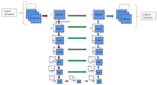
Figure 1.
Schematic of the CNN architecture. Each blue box represents a multichannel feature map generated by the last convolutional layer. The generating matrix size is denoted in the box. Green arrows denote “skip-connections” via concatenation.
The U-net architecture used in this paper is symmetrical, which means the encoding and decoding processes have the same depth, and the corresponding blocks are identified. The left side of the architecture is the encoding process, in which the values of the temperature field are progressively down-sampled using convolutional calculations. The encoding process is used for recognizing the geometry and the boundary conditions of the physical input field to extract the necessary features using a convolution operation layer-by-layer. The square filters are applied to conduct the convolutional calculation layer-by-layer until the matrices with only one data point are obtained (see the block at the vertex of the triangle structure). In this approach, the large-scale information can be extracted as the feature channels, which increase through layers. The decoding part, which corresponds to the right side of the structure, is an inverse convolutional process and mirrors the operations of the encoding part. By decreasing the feature channel amounts and increasing spatial resolution, the solutions of the temperature field are reconstructed in the up-sampling layers. As shown in the Figure 1, the horizontal and vertical arrows concatenate the encoding and corresponding decoding blocks [44]. The motivation of these connections is doubling the feature channels of the decoding block, which are connected by green horizontal arrows, and making the neural networks consider the information from the encoding layers connected by red and blue vertical arrows.
To train the CNNs, stochastic gradient descent optimization is used, which needs a loss function to calculate the difference between the results and the ground truth. Furthermore, in each epoch, the weights of every convolutional block are updated with the Adam optimizer during the backpropagation process [48].
3.2. Physics-Driven Training Approach
Recently, the physics-driven training methods for deep learning have shown particular promise for the physical field prediction work for their advantages that reduce the heavy requirement of a large amount of training data [49]. In the typical data-driven method, the mathematical formulation of the loss function compares the difference between the prediction result and the ground truth as:
As shown in Equation (1), the subscript “data” denotes data-driven, and the , are output and true temperature fields, respectively. In this paper, the loss function is built based on Fourier’s law. The physics law of heat conduction can be expressed with a second-order PDE, the Laplace equation. The system assumes no inner heat source contribution, and the thermal conductivity is considered constant. Under this assumption, the physical law of heat conduction can be expressed with a second-order PDE Laplace equation. the two-dimensional form is defined as shown in Equation (2):
In the physics-driven method, the Laplace equation is used to drive the training process as the loss function, as shown in Equation (3):
The Dirichlet boundary conditions are applied in the temperature field, where the temperatures of the outer and inner of the plate are constant at zero degrees.
As proposed previously for simple PDEs [50], the Laplace equation can be calculated through finite differences using suitable convolutional filters. The backpropagation of the loss can be achieved with convolutions. The weights of the first- and second-order differential kernels are shown in Equation (4):
The multiple cases training is shown in Figure 2. Ten temperature fields and ten masks are the two inputs of the U-net architecture. Then, the backpropagation process calculates the loss function’s gradient and updates the multilayer CNN’s weights to satisfy the loss function, which is the residual of the Laplace equation. Finally, when the threshold of the loss function is reached, accurate field solutions are generated.
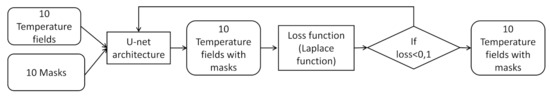
Figure 2.
The physics-driven training approach. One batch has ten layout masks.
3.3. PSO Algorithm
The particle swarm optimization (PSO) algorithm is inspired by groups of birds. The basic idea is to collaborate and share between individual birds in the group to find the optimal solution [51]. PSO has been selected in this research, which is a computational method that optimizes a problem by iteratively trying to improve a candidate solution with regard to a given measure of quality.
PSO is a new evolutionary algorithm developed in recent years. Similar to the simulated annealing algorithm, PSO starts from a random solution and finds the optimal solution through iteration. It also evaluates the quality of the solution through fitness but has simpler rules than the genetic algorithm. PSO does not have the “crossover” and “mutation” operations of the genetic algorithm. It finds the global optimum by following the current searched optimum value. The algorithm of PSO is easy to implement, has high precision, and has fast convergence. It is also a parallel algorithm, that is, a a neural network algorithm with great potential. The PSO algorithm was proposed because of its intuitive background, simplicity, easy implementation, and wide adaptability to different types of functions. The PSO algorithm has good performance in many fields, such as power systems, biological information, logistics planning, etc. At present, the standard particle swarm algorithm is very mature and has standard test functions in many different dimensions, ranging from accuracy (deviation from the optimal solution), success rate (probability of computing to the optimal solution), computational speed, stability (mean, median, variance), etc. The algorithms were tested and achieved good results [52,53,54].
The feasibility of this method has been proved in many scientific and industrial fields [55,56,57,58,59,60,61]. PSO requires a solution space conventionally achieved by discrete methods by optimizing the algorithms. There are multiple boundary conditions and multiple inputs when considering complex optimization goals. The effort of accompanying numerical simulations is usually prohibitive [62]. The particle swarm optimization (PSO) algorithm is an emerging optimization technology whose ideas originate from artificial life and evolutionary computing theory. Particle swarm optimization completes the optimization by the particles following the best solution found by themselves and the best solution of the entire swarm. Compared with other evolutionary algorithms, this algorithm is simple and easy to implement, has few adjustable parameters, has stronger global optimization ability, and has been widely studied and applied [63,64]. Similar to the simulated annealing algorithm, PSO starts from a random solution and finds the optimal solution through iteration. It also evaluates the quality of the solution through fitness but has simpler rules than the genetic algorithm. PSO does not have the “crossover” and “mutation” operations of the genetic algorithm. It finds the global optimum by following the currently searched optimum value.
In this paper, the PD-CNN surrogate model calculates the solutions inside the domain effectively. Given a precise layout and boundary condition, the model can directly output the corresponding temperature distribution, significantly reducing the computational workload. The PD-CNN replaces the numerical analysis tool by constructing a high-precision model and has achieved a compromise between calculation accuracy and computational cost, thereby improving the optimization’s efficiency. It is straightforward to guide the numerical algorithm to solve the optimization problem in a limited time.
The PSO process is shown in Figure 3. As introduced above, the birds involve placing several simple things called particles. Each particle evaluates the fitness at its present location in the space of a problem or function. By combining some aspect of the history of the swarm’s fitness values with those of one or more swarm members, each particle can determine its movement through the parameter space. Then, by the locations and processed fitness values of those other members, along with random perturbations, the swarm can move through the parameter space with a determined velocity. The swarm members can interact with their neighborhoods and the colonial neighborhoods of all particles in a PSO network.
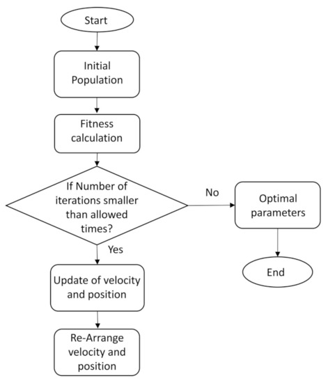
Figure 3.
Schematic of the PSO method.
The objective of the optimization is to minimize the mean temperature value through the whole precise domain. The machine learning methods can predict the temperature distribution of multiple cases simultaneously. So, in every epoch, ten initial temperature fields with ten different layouts are input into the U-net structure. The restriction condition is the total area of the hole. There are three different study cases as shown in Table 1:

Table 1.
Study cases.
In the first case, the hole position of the mask is located at the exact center of the entire computational domain, the coordinates are (64, 64), and the area of the hole is fixed as 400. The side length of the hole can be changed, ranging from 5 to 80. In the second case, the side length of the hole is fixed at 20 × 10. The area of the hole is 200. The center position of each hole can be moved up, down, left, and right, and the moving size is 1, 5, and 10 pixels in each epoch. For the third case, the side length of the hole is fixed at 10 × 10. The area of the hole is 100. The center position of each hole is defined as Case 2, which can be moved up, down, left, and right, and the moving size is 1, 5, and 10 pixels in each epoch. As described above, PSO simulates the predatory the behavior of a flock of birds. Imagine a scenario where a group of birds is randomly searching for food. There is only one piece of food in this area; the birds do not know where the food is, but they know how good the current location is (the closer the location to the food, the better). So, what is the optimal strategy for finding food? The easiest and most effective is to search the area around the bird that is currently closest to the food. During the whole search process, the birds pass their respective information to each other so that other birds know their position. In the end, the whole flock can gather around the food source; that is, the optimal solution is found. In PSO, the position of each bird is a solution in the solution space of the optimization problem. We call them “particles”. All particles have a fitness value determined by the function being optimized, and each particle also has a velocity that determines the direction and rate at which they fly. Then, the particles follow the current optimal particle to search in the solution space. In the initialization phase, PSO generates a group of random particles (i.e., random solutions) and then iteratively finds the optimal solution. In each iteration, the particle updates itself by tracking two “extremes”. The first extreme value is the historical optimal solution found by the particle itself, and this solution is called the individual extreme value pBest. The other extreme value is the historical optimal solution found by the entire population, and this extreme value is the global extreme value gBest.
4. PD-CNN Model Training
The CNN surrogate model, which is shown in Figure 4, is used for the optimization tasks described in the next section. The finite element method FEM model can provide an accurate temperature prediction for heat transfer. However, the optimization based on the FEM model could be infeasible, as discussed above. The FEM can only provide solutions with precise boundary conditions and layouts. Therefore, the result is not given in an explicit form. The PD-CNN model, in contrast, is an accurate mapping between the layouts and corresponding solutions and can predict the temperature distribution for any randomly given geometry. Therefore, a CNN surrogate model could be a suitable choice for layout optimization. Figure 4 shows the input and output of the CNN surrogate model in the case of four holes. Ten randomly generated masks are used as the input for the CNN surrogate model during every epoch. The masks also change with different epochs.
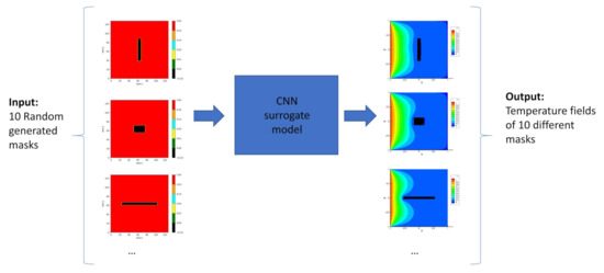
Figure 4.
The temperature distribution prediction using the trained PD-CNN surrogate model.
As shown in Figure 5a, the Laplace residual value drops exponentially in the beginning; after approximately 20 iterative steps, the convergence of the Laplace residual exhibits minor differences. When the iterative training step reaches 500k, the value decreases to be sufficiently small. After then, the Laplace residual oscillates around 0.35, as shown in Figure 5b, which is considered converged. The whole converge curve is very similar to the curve using the combined data- and physics-driven the method in Ref. [41]. The training process with 500,000 epochs requires around 9 h using the following device: Intel Core i5-10300H CPU and NVIDIA GeForce RTX 2060.
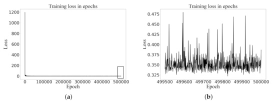
Figure 5.
Convergence curve. (a) Iterative steps: 1–500 k; (b) Iterative steps: 499,500–500 k.
The training process is shown in Figure 6. Here, 100,000 are set as the maximal epochs, In each generation, the GPU trains ten different cases as one batch, and the learning rate is specified as 0.001. The positions of masks in each epoch are randomly generated. The PD-CNN is used to obtain the solutions to multiple cases with a unique surrogate model. The input masks are varied in a moderate range in the training stage. The fixed network can generate the corresponding temperature field. The setup of the mask position is shown in Table 1, as discussed earlier. Training loss is relatively significant at the beginning of the training process, and there are many errors in local temperature fields. These inconsistency errors show a significant Laplace loss, which cannot predict the temperature field very well. As the epochs increase, the inconsistency of the temperature field decreases, and the results seem to be more reasonable, shown in Figure 6 The training loss decreases very fast at first and then keeps stable. Although the loss does not decrease, the results keep becoming better after 10,000 epochs. In the end, the model adapts to the random size of different masks, which completely covers the surrogate model’s range.
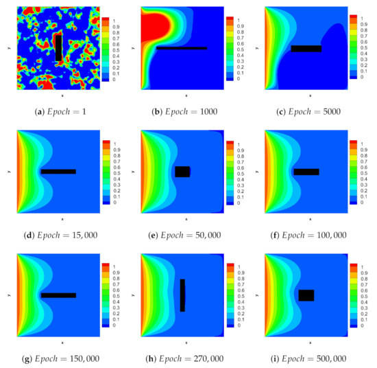
Figure 6.
The training evolution of temperature field solution from epoch 0 to 500,000 for the single hole case.
As shown in Figure 6, the mask changes in every epoch in the learning process, and the contours of the temperature field become smoother. As the advantage of physics-driven learning, the relation of adjacent points is constrained by the Laplace equation. For this reason, the values do not vary dramatically. Then in epoch 1000, a significant error spot appears, denoted as a peak in which the value is round 3, see Figure 6b, and the residuals near the domain’s boundaries are negative. The whole temperature field is much different from the proper solution. Finally, from epoch 15,000, the global structure is stable and very similar to the proper solution after the gradual disappearance of the peaks. However, there are still residuals near the boundaries of holes, which is a specific numerical solution to an unsteady heat conduction problem with a Dirichlet boundary condition [41]. In the validation phase, the surrogate model can predict the temperature field immediately. As the results presented in the next section, the prediction of the PD-CNN surrogate model is almost identical to numerical simulation results.
5. Prediction and Optimization
This section shows the prediction results of the temperature field with a single-hole mask and multiplied holes mask. Then, the optimization results are shown and discussed in detail in this section. Finally, the results from the PD-CNN method are compared with FEM simulation results.
5.1. Shape Optimization in the Single-Hole Case
The single mask dimension is optimized with the PSO method, and the corresponding temperature field is shown and discussed.
The area of every hole is fixed as 400, and every side length of the hole is variable in the range from 5 to 80. The mask is at the central position of the whole domain. After the PSO optimization process using a PD-CNN surrogate model, the temperature field with the optimized mask is shown in Figure 7a. The width of the optimized mask is 5, and the height is 80. The mask has divided the temperature field into upper and lower parts. According to Table 2, the mask’s width should be as small as possible to reduce the heat transfer from the left to the right. With this optimized mask, the mean temperature of the whole area is at a minimum. Figure 7b is the result from FEM, which is considered as the proper reference. The result of the PD-CNN has shown significant performance.
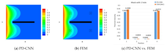
Figure 7.
Comparison between surrogate model prediction and FEM result for the one-hole case: (a): temperature field with an optimized mask using a CNN surrogate model; (b): temperature field with an optimized cover using the FEM method; (c): quantitative comparison of the two results.
Table 2.
The shape optimization of the 1-hole case.
For quantitative analysis, four square sampling areas are marked in the temperature field obtained by the two methods. The length of each side of the square is 5, and the distance from the center point to the boundary is 20. The temperature values in each square are averaged. The difference between the two results can be intuitively observed and compared, as shown in Figure 7c. It can be seen from the histogram that the difference between the results obtained by the PD-CNN method and the FEM method in sampling areas one and four is more significant than that in sampling areas two and three. The possible reason is that the heat source is located on the left boundary, the temperature is transmitted from the left to the right, the value changes significantly in the area close to the left, and the calculation results are slower to converge, which leads to more significant errors. The results of sampling areas two and three are on the right. Again, the difference between the numerical and reference numerical values is slight. The reason is that the heat source propagation is blocked due to the blocking of the hole so that the numerical value on the right side of the cavity changes less, the calculation converges more quickly, and the difference is minor.
5.2. Position Optimization in the Multiple-Holes Cases
For the temperature field with two masks, each area is fixed as , and the central position of each hole is movable from the center of the whole domain, which is . The movement of both coordinates, x and y, is from −10 to 10.
Figure 8a shows the temperature field with two optimized masks. The area of each mask is fixed as 20 × 10. The central coordinate of each mask is movable inside the domain. Before optimization, two masks were in the same position (64, 64). The movement of each mask’s coordinate x and y ranges from −10 to 10. Table 3 shows the coordinate of masks after optimization. One mask was moved to the left upper part, while another was moved to the left lower part. In this situation, the square plate has the minimum mean temperature. Figure 8b is the result from FEM, which is defined as the proper reference. Analyzing from a qualitative perspective, the result from the PD-CNN has a good agreement with that of FEM.
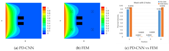
Figure 8.
Comparison between surrogate model prediction and FEM result for the two-holes case. (a): Temperature field with an optimized mask using a CNN surrogate model; (b): Temperature field with an optimized cover using the FEM method; (c): quantitative comparison of the two results.
Table 3.
The position optimization of the two-holes case.
We can observe a similar result in this case compared with the one-hole case. The difference between the sampling area near the heat source and the reference value is greater than the difference between the sampling area on the right side of the mask.
Figure 9a shows the temperature field with four optimized masks using the PD-CNN method. The area of each hole is fixed as 10 × 10, and the central position of each hole is movable from the center of the plate. Four masks were in the same position, which means they were coincident initially. The movement of each mask’s coordinate x and y ranges from −20 to 20. We notice that three holes are arranged vertically in the middle and left part of the entire domain, and the fourth mask is located on the right and upper of the whole field as shown in Table 4. Considering the symmetry of the computational domain, we can easily infer the distribution of another solution: the top hole is on the right upper side. In addition, in this case, we can see the numerical difference distribution similar to the previous two instances from Figure 9c. The only difference is that the temperature values obtained by the PD-CNN have residuals in the four corners. The reason is that the calculation is more complicated in the case of four holes, and the convergence speed will decrease. Still, as the number of training increases, this residual will gradually disappear.
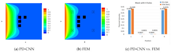
Figure 9.
Comparison between surrogate model prediction and FEM result for four-holes case: (a): temperature field with an optimized mask using a CNN surrogate model; (b): temperature field with an optimized cover using the FEM method; (c): quantitative comparison of the two results.
Table 4.
The position optimization of the four-holes case.
In the above three cases, the results obtained by the traditional FEM method were used as the references, and the difference between results obtained by the PD-CNN method and the results obtained by the FEM method were compared, which proved from a qualitative point of view the high effectiveness of the new process. From a quantitative point of view, the article compares the difference in the numerical average of the results obtained by the two methods in four different specific areas, which verifies the high accuracy of the new method. The numerical simulation method based on a finite element is widely used in the analysis and evaluation of the temperature field. However, if the analysis program is called repeatedly during the optimization design process, the calculation cost will be too high, and the optimization cost will be huge, and even the design task cannot be completed in a limited time. Our new method mainly replaces the high-precision model by constructing an approximate model (also called a surrogate model) to achieve a compromise between computational accuracy and computational cost, thereby improving the solution efficiency. The computational cost problem is solved.
6. Discussion
This paper investigates the approximate modeling task of the temperature field in the process of heat-conduction-temperature field optimization, focusing on exploring the approximate modeling method of building a surrogate model based on a deep neural network, realizing near real-time prediction of the temperature field, and forming a complete set of heat conduction data sets, benchmark models, and evaluation criteria for temperature field prediction studies. At the same time, an optimization approach was employed to forecast heat transmission. This approach is projected to be used to approximate modeling problems in other physical disciplines (force, electromagnetic, etc.) in the future and has extensive application potential. The physics-driven approach is significantly quicker than the conventional data-driven method for approximating real solutions. This approach decreases the high data generation cost of data-driven approaches, since the objectives only comprise a limited number of examples and are used throughout the whole training process. The reference objectives in practical engineering applications may be simply selected from existing data, such as experimental and numerical data. The training samples used in the loss function may be difficult to obtain for complicated actual engineering situations. In contrast, the physics-driven method trains the model to solve the physics field without using labeled data. Two significant scientific topics were chosen to examine the physics-driven technique in papers [37,41]. In [37], the physical constraints are applied to the preliminary flow field derived from the U-net CNN generator for the flow around a cylinder issue.
7. Conclusions
In this paper, we proposed an optimization framework based on the PSO algorithm and the PD-CNN surrogate model for the layout of a heat conducting plate. The Laplace equation was utilized as a loss function during the learning process. The U-net structure CNN was trained to predict the accurate temperature solution of the precise layouts without any training data. The PSO algorithm was used to obtain the optimized shape and position of the heat insulation holes in the single and multiple holes optimization. The solution predictions have significant similarities with the FEM results. The proposed approach achieved promising results for thermal intensity. This optimization framework is helpful for practical application when the training data are not accurate. It is noteworthy that the U-net architecture using CNN is suitable for general physics laws, which can be expressed as PDEs. As a result of applying the physics-driven-based approach, the learning process may be significantly accelerated even with relatively unrestricted selections of reference targets, which is important for practical application when an accurate reference is unavailable. It is worth mentioning that the associated CNN architecture and heat conduction problem are universal, and the PD-CNN approach applies to various physical laws written as PDEs. Further study will be conducted to anticipate complicated flow fields using the current method. In the future, multiscale CNN architecture will be investigated for complicated prediction. Indeed, challenging aerodynamic optimization will be studied to improve the research results. In addition to that, we will compare the proposed approach with different methods to validate the performance and reliability of the architecture.
Author Contributions
Methodology, Y.S., A.E., H.M. and M.R.C. All authors have read and agreed to the published version of the manuscript.
Funding
This research received no external funding.
Informed Consent Statement
Not applicable.
Data Availability Statement
Not applicable.
Acknowledgments
Hao Ma (No. 201703170250) was supported by China Scholarship Council when he conducted the work this paper represents. Yang Sun is supported by the Europe Erasmus Exchange Program at the Technical University of Munich (TUM), Germany. We thank the Islamic Development Bank for their support to the Ph.D. work of A. Elhanashi. The author thanks the colleagues of TUM and the University of Pisa (UNIPI) for the beneficial discussions.
Conflicts of Interest
The authors declare no conflict of interest.
References
- Bendsoe, M.P.; Sigmund, O. Topology Optimization: Theory, Methods, and Applications; Springer Science & Business Media: Berlin, Germany, 2003. [Google Scholar]
- Chen, K.; Wang, S.; Song, M. Optimization of the heat source distribution for two-dimensional heat conduction using the bionic method. Int. J. Heat Mass Transf. 2016, 93, 108–117. [Google Scholar] [CrossRef]
- Hughes, T.J. The Finite Element Method: Linear Static and Dynamic Finite Element Analysis; Courier Corporation: North Chelmsford, MA, USA, 2012. [Google Scholar]
- Gu, Y.; Wang, L.; Chen, W.; Zhang, C.; He, X. Application of the meshless generalized finite difference method to inverse heat source problems. Int. J. Heat Mass Transf. 2017, 108, 721–729. [Google Scholar] [CrossRef]
- Chen, X.; Chen, X.; Zhou, W.; Zhang, J.; Yao, W. The heat source layout optimization using deep learning surrogate modeling. Struct. Multidiscip. Optim. 2020, 62, 3127–3148. [Google Scholar] [CrossRef]
- Lei, X.; Liu, C.; Du, Z.; Zhang, W.; Guo, X. Machine learning-driven real-time topology optimization under moving morphable component-based framework. J. Appl. Mech. 2019, 86, 011004. [Google Scholar] [CrossRef]
- Brunton, S.L.; Noack, B.R.; Koumoutsakos, P. Machine learning for fluid mechanics. Annu. Rev. Fluid Mech. 2020, 52, 477–508. [Google Scholar] [CrossRef]
- Ma, H.; Zhang, Y.x.; Haydn, O.J.; Thuerey, N.; Hu, X.y. Supervised learning mixing characteristics of film cooling in a rocket combustor using convolutional neural networks. Acta Astronaut. 2020, 175, 11–18. [Google Scholar] [CrossRef]
- Ma, H.; Zhang, B.; Zhang, C.; Haidn, O.J. Generative adversarial networks with physical evaluators for spray simulation of pintle injector. AIP Adv. 2021, 11, 075007. [Google Scholar] [CrossRef]
- Hughes, M.T.; Kini, G.; Garimella, S. Status, challenges, and potential for machine learning in understanding and applying heat transfer phenomena. J. Heat Transf. 2021, 143, 120802. [Google Scholar] [CrossRef]
- Farimani, A.B.; Gomes, J.; Pande, V.S. Deep learning the physics of transport phenomena. arXiv 2017, arXiv:1709.02432. [Google Scholar]
- Tanaka, A.; Tomiya, A.; Hashimoto, K. Deep Learning and Physics; Springer: Berlin/Heidelberg, Germany, 2021. [Google Scholar]
- Bourilkov, D. Machine and deep learning applications in particle physics. Int. J. Mod. Phys. A 2019, 34, 1930019. [Google Scholar] [CrossRef]
- Carleo, G.; Cirac, I.; Cranmer, K.; Daudet, L.; Schuld, M.; Tishby, N.; Vogt-Maranto, L.; Zdeborová, L. Machine learning and the physical sciences. Rev. Mod. Phys. 2019, 91, 045002. [Google Scholar] [CrossRef]
- Saponara, S.; Elhanashi, A.; Gagliardi, A. Exploiting R-CNN for video smoke/fire sensing in antifire surveillance indoor and outdoor systems for smart cities. In Proceedings of the 2020 IEEE International Conference on Smart Computing (SMARTCOMP), Bologna, Italy, 14–17 September 2020; pp. 392–397. [Google Scholar] [CrossRef]
- Saponara, S.; Elhanashi, A.; Zheng, Q. Recreating fingerprint images by convolutional neural network autoencoder architecture. IEEE Access 2021, 9, 147888–147899. [Google Scholar] [CrossRef]
- Bekkerman, R.; Bilenko, M.; Langford, J. Scaling Up Machine Learning: Parallel and Distributed Approaches; Cambridge University Press: Cambridge, UK, 2011. [Google Scholar]
- Mitchell, T.; Buchanan, B.; DeJong, G.; Dietterich, T.; Rosenbloom, P.; Waibel, A. Machine learning. Annu. Rev. Comput. Sci. 1990, 4, 417–433. [Google Scholar] [CrossRef]
- Yan, W.; Lin, S.; Kafka, O.L.; Lian, Y.; Yu, C.; Liu, Z.; Yan, J.; Wolff, S.; Wu, H.; Ndip-Agbor, E.; et al. Data-driven multi-scale multi-physics models to derive process–structure-property relationships for additive manufacturing. Comput. Mech. 2018, 61, 521–541. [Google Scholar] [CrossRef]
- Zhang, Z.J.; Duraisamy, K. Machine learning methods for data-driven turbulence modeling. In Proceedings of the 22nd AIAA Computational Fluid Dynamics the conference, Dallas, TX, USA, 22–26 June 2015; p. 2460. [Google Scholar]
- Kirchdoerfer, T.; Ortiz, M. Data-driven computational mechanics. Comput. Methods Appl. Mech. Eng. 2016, 304, 81–101. [Google Scholar] [CrossRef]
- Christelis, V.; Mantoglou, A. Physics-based and data-driven surrogate models for pumping optimization of coastal aquifers. Eur. Water 2017, 57, 481–488. [Google Scholar]
- Kim, M.; Pons-Moll, G.; Pujades, S.; Bang, S.; Kim, J.; Black, M.J.; Lee, S.H. Data-driven physics for human soft tissue animation. ACM Trans. Graph. (TOG) 2017, 36, 1–12. [Google Scholar] [CrossRef]
- Schmid, P.J. Dynamic mode decomposition of numerical and experimental data. J. Fluid Mech. 2010, 656, 5–28. [Google Scholar] [CrossRef]
- Anzai, Y. Pattern Recognition and Machine Learning; Elsevier: Amsterdam, The Netherlands, 2012. [Google Scholar]
- Sosnovik, I.; Oseledets, I. Neural networks for topology optimization. Russ. J. Numer. Anal. Math. Model. 2019, 34, 215–223. [Google Scholar] [CrossRef]
- Müller, J.; Park, J.; Sahu, R.; Varadharajan, C.; Arora, B.; Faybishenko, B.; Agarwal, D. Surrogate optimization of deep neural networks for groundwater predictions. J. Glob. Optim. 2020, 81, 203–231. [Google Scholar] [CrossRef]
- There, N.; Weißenow, K.; Prantl, L.; Hu, X. Deep learning methods for Reynolds-averaged Navier–Stokes simulations of airfoil flows. AIAA J. 2020, 58, 25–36. [Google Scholar] [CrossRef]
- Bhatnagar, S.; Afshar, Y.; Pan, S.; Duraisamy, K.; Kaushik, S. Prediction of aerodynamic flow fields using convolutional neural networks. Comput. Mech. 2019, 64, 525–545. [Google Scholar] [CrossRef]
- Chen, J.; Viquerat, J.; Hachem, E. U-net architectures for fast prediction of incompressible laminar flows. arXiv 2019, arXiv:1910.13532. [Google Scholar]
- Tao, J.; Sun, G. Application of deep learning-based multi-fidelity surrogate model to robust aerodynamic design optimization. Aerosp. Sci. Technol. 2019, 92, 722–737. [Google Scholar] [CrossRef]
- del Rio-Chanona, E.A.; Wagner, J.L.; Ali, H.; Fiorelli, F.; Zhang, D.; Hilliard, K. Deep learning-based surrogate modeling and optimization for microalgal biofuel production and photobioreactor design. AIChE J. 2019, 65, 915–923. [Google Scholar] [CrossRef]
- Eismann, S.; Bartzsch, S.; Ermon, S. Shape optimization in laminar flow with a label-guided variational autoencoder. arXiv 2017, arXiv:1712.03599. [Google Scholar]
- Li, J.; Zhang, M.; Martins, J.R.; Shu, C. Efficient aerodynamic shape optimization with deep-learning-based geometric filtering. AIAA J. 2020, 58, 4243–4259. [Google Scholar] [CrossRef]
- Chen, L.W.; Cakal, B.A.; Hu, X.; Thuerey, N. Numerical investigation of minimum drag profiles in laminar flow using deep learning surrogates. J. Fluid Mech. 2021, 919, A34. [Google Scholar] [CrossRef]
- Wang, Y.; Wang, W.; Tao, G.; Li, H.; Zheng, Y.; Cui, J. Optimization of the semi-sphere vortex generator for film cooling using the generative adversarial networks. Int. J. Heat Mass Transf. 2022, 183, 122026. [Google Scholar] [CrossRef]
- Ma, H.; Zhang, Y.; Thuerey, N.; Hu, X.; Haidn, O.J. Physics-driven learning of the steady Navier-Stokes equations using deep convolutional neural networks. arXiv 2021, arXiv:2106.09301. [Google Scholar] [CrossRef]
- Raissi, M.; Perdikaris, P.; Karniadakis, G.E. Physics informed deep learning (part i): Data-driven solutions of nonlinear partial differential equations. arXiv 2017, arXiv:1711.10561. [Google Scholar]
- Zhu, Y.; Zabaras, N.; Koutsourelakis, P.S.; Perdikaris, P. Physics-constrained deep learning for high-dimensional surrogate modeling and uncertainty quantification without labeled data. J. Comput. Phys. 2019, 394, 56–81. [Google Scholar] [CrossRef]
- Geneva, N.; Zabaras, N. Modeling the dynamics of PDE systems with physics-constrained deep auto-regressive networks. J. Comput. Phys. 2020, 403, 109056. [Google Scholar] [CrossRef]
- Ma, H.; Hu, X.; Zhang, Y.; Thuerey, N.; Haidn, O.J. A Combined Data-driven and Physics-driven Method for Steady Heat Conduction Prediction using Deep Convolutional Neural Networks. arXiv 2020, arXiv:2005.08119. [Google Scholar]
- Lu, L.; Meng, X.; Mao, Z.; Karniadakis, G.E. DeepXDE: A deep learning library for solving differential equations. SIAM Rev. 2021, 63, 208–228. [Google Scholar] [CrossRef]
- Sun, L.; Gao, H.; Pan, S.; Wang, J.X. Surrogate modeling for fluid flows based on physics-constrained deep learning without simulation data. Comput. Methods Appl. Mech. Eng. 2020, 361, 112732. [Google Scholar] [CrossRef]
- Ronneberger, O.; Fischer, P.; Brox, T. U-net: Convolutional networks for biomedical image segmentation. In Proceedings of the International Conference on Medical image Computing and Computer-Assisted Intervention, Munich, Germany, 5–9 October 2015; Springer: Berlin/Heidelberg, Germany, 2015; pp. 234–241. [Google Scholar]
- Paszke, A.; Gross, S.; Massa, F.; Lerer, A.; Bradbury, J.; Chanan, G.; Killeen, T.; Lin, Z.; Gimelshein, N.; Antiga, L.; et al. Pytorch: An imperative style, high-performance deep learning library. Adv. Neural Inf. Process. Syst. 2019, 32, 8026–8037. [Google Scholar]
- Yamashita, R.; Nishio, M.; Do, R.K.G.; Togashi, K. Convolutional neural networks: An overview and application in radiology. Insights Imaging 2018, 9, 611–629. [Google Scholar] [CrossRef]
- Ruder, S. An overview of gradient descent optimization algorithms. arXiv 2016, arXiv:1609.04747. [Google Scholar]
- Kingma, D.P.; Ba, J. Adam: A method for stochastic optimization. arXiv 2014, arXiv:1412.6980. [Google Scholar]
- Lim, J.; Psaltis, D. MaxwellNet: Physics-driven deep neural network training based on Maxwell’s equations. APL Photonics 2022, 7, 011301. [Google Scholar] [CrossRef]
- Sharma, R.; Farimani, A.B.; Gomes, J.; Eastman, P.; Pande, V. Weakly-supervised deep learning of heat transport via physics informed loss. arXiv 2018, arXiv:1807.11374. [Google Scholar]
- Kennedy, J.; Eberhart, R. Particle swarm optimization. In Proceedings of the ICNN’95-International Conference on Neural Networks, Perth, WA, Australia, 27 November–1 December 1995; Volume 4, pp. 1942–1948. [Google Scholar]
- Yang, X.S.; Deb, S. Cuckoo search via Lévy flights. In Proceedings of the 2009 World Congress on Nature & Biologically Inspired Computing (NaBIC), Coimbatore, India, 9–11 December 2009; pp. 210–214. [Google Scholar]
- Li, X.l. An optimizing method based on autonomous animats: Fish-swarm algorithm. Syst. Eng.-Theory Pract. 2002, 22, 32–38. [Google Scholar]
- Zhang, H.; Yuan, M.; Liang, Y.; Liao, Q. A novel particle swarm optimization based on prey-predator relationship. Appl. Soft Comput. 2018, 68, 202–218. [Google Scholar] [CrossRef]
- Sterling, A. Review of handbook of nature-inspired and innovative computing by Albert Y. Zomaya. ACM SIGACT News 2011, 42, 23–26. [Google Scholar] [CrossRef]
- Kennedy, J. Swarm intelligence. In Handbook of Nature-Inspired and Innovative Computing; Springer: Berlin/Heidelberg, Germany, 2006; pp. 187–219. [Google Scholar]
- Eberhart; Shi, Y. Particle swarm optimization: Developments, applications, and resources. In Proceedings of the 2001 Congress on Evolutionary Computation (IEEE Cat. No. 01TH8546), Seoul, Korea, 27–30 May 2001; Volume 1, pp. 81–86. [Google Scholar]
- Sigmund, O. A 99-line topology optimization code written in Matlab. Struct. Multidiscip. Optim. 2001, 21, 120–127. [Google Scholar] [CrossRef]
- Bendsøe, M.P.; Kikuchi, N. Generating optimal topologies in structural design using a homogenization method. Comput. Methods Appl. Mech. Eng. 1988, 71, 197–224. [Google Scholar] [CrossRef]
- Mlejnek, H.P.; Schirrmacher, R. An engineer’s approach to optimal material distribution and shape finding. Comput. Methods Appl. Mech. Eng. 1993, 106, 1–26. [Google Scholar] [CrossRef]
- Huang, X.; Xie, M. Evolutionary Topology Optimization of Continuum Structures: Methods and Applications; John Wiley & Sons: Hoboken, NJ, USA, 2010. [Google Scholar]
- Mueller, L.; Verstraete, T. Adjoint-based multi-point and multi-objective optimization of a turbocharger radial turbine. Int. J. Turbomach. Propuls. Power 2019, 4, 10. [Google Scholar] [CrossRef]
- Milani, A.; Santucci, V.; Leung, C. Optimizing web content presentation: A online PSO approach. In Proceedings of the 2009 IEEE/WIC/ACM International Joint Conference on Web Intelligence and Intelligent Agent Technology, Milan, Italy, 15–18 September 2009; Volume 3, pp. 26–29. [Google Scholar]
- Niasar, N.S.; Shanbezade, J.; Perdam, M.; Mohajeri, M. Discrete fuzzy particle swarm optimization for solving traveling salesman problem. In Proceedings of the 2009 International Conference on Information and Financial Engineering, Singapore, 17–20 April 2009; pp. 162–165. [Google Scholar]


Publisher’s Note: MDPI stays neutral with regard to jurisdictional claims in published maps and institutional affiliations. |
© 2022 by the authors. Licensee MDPI, Basel, Switzerland. This article is an open access article distributed under the terms and conditions of the Creative Commons Attribution (CC BY) license (https://creativecommons.org/licenses/by/4.0/).