Similarity-Based Malware Classification Using Graph Neural Networks

Abstract

This work proposes a novel malware identification model that is based on a graph neural network (GNN). The function call relationship and function assembly content obtained by analyzing the malware are used to generate a graph that represents the functional structure of a malware sample. In addition to establishing a multi-classification model for predicting malware family, this work implements a similarity model that is based on Siamese networks, measuring the distance between two samples in the feature space to determine whether they belong to the same malware family. The distance between the samples is gradually adjusted during the training of the model to improve the performance. A Malware Bazaar dataset analysis reveals that the proposed classification model has an accuracy and area under the curve (AUC) of 0.934 and 0.997, respectively. The proposed similarity model has an accuracy and AUC of 0.92 and 0.92, respectively. Further, the proposed similarity model identifies the unseen malware family with approximately 70% accuracy. Hence, the proposed similarity model exhibits better performance and scalability than the pure classification model and previous studies.

1. Introduction

G DATA’s 2020 Threat Analysis Report [1] stated that cybercriminals have relied on malicious software for many years, and such software is being continuously developed. According to AV Test’s 2019/2020 Security Report [2], of 114 million pieces of new malware, 78.64% were distributed on Windows systems. In 2019, Microsoft reported over 660 Windows vulnerabilities in the CVE^® database. The COVID-19 pandemic increased the need to work remotely, and the proportion of malware that has been distributed on Windows systems has increased to 83.45% in the last year. Most methods of malware identification involve reverse engineering to analyze the features of the malware. The reverse engineering of malware involves decompiling and disassembling a software program. In these processes, binary object files are converted to higher-level constructs so that engineers can look at the program’s function and extract important information provided by embedded resources in the malware, encryption keys, details of the loader, header, metadata, and so on. Usually, analyzing a program inside a file by reverse engineering takes considerable time. Additionally, some files may be incomplete or grammatically incorrect code snippets that cannot be compiled, greatly increasing the time required to investigate a file. Analysis of an obfuscated file and inability to disassemble binary files are difficult problems to solve in reverse engineering. Therefore, determining whether each file is good or bad by reverse engineering takes a long time and requires many human resources to complete. In this work, graph neural networks (GNN) with function embedding techniques are used to classify malware into families. Similarity analyses between malware codes must typically be conducted as part of the malware analysis to determine the relationship between two malware samples. However, malicious codes within a single malware family can greatly differ, such that they are treated as different categories in feature space. Therefore, this research proposes the training of a similarity model using a Siamese network to merge the features of codes in the same malware family into a single group of features. This procedure can reduce the time that must be spent by an expert in analyzing a malware sample.

The GNN model and the Siamese model both have the feature vector after data construction as inputs. Although both models can classify malware, these two approaches have different purposes and applications. The GNN classification model is limited to classifying malware with which it has been trained; the model must be retrained to recognize malware of a new category. In contrast, the similarity model calculates the similarity between samples. The category that is most similar to that of a new sample can be determined by calculating the distance between two feature vectors.

The main contributions of this research are summarized as follows:

• We proposed a method for transforming malware behavior into a graph data structure; the transforming method disassembles raw execution files into code and then transforms the functions into nodes to build a graph.
• We developed graph neural network models to identify malware families; the generated graphs are fed into a graph neural network so that the network learns the code structure to identify malware families.
• We visualized graph embedding of a similarity model; the graph is visualized to prove that after the malware is trained, the malware families can be grouped.
• Compared with previous studies, experimental results reveal that this research can effectively identifies malware.

The first section of the paper explores the statistics about the cyberattacks landscape, malware detection, and malware distribution. The second section introduces malware concept, malware analysis, and malware detection-related studies. The third section is the architecture of the malware family classification and similarity system. The fourth section describes system implementation and performance analysis. The last section is the conclusions of this study.

2. Malware Detection and Classification Techniques

Malware is a contraction of malicious software, which refers to a program that intentionally damages computers or steals confidential information over the Internet or from a portable device. Pieces of malware have various behaviors and purposes. They include viruses, Trojan horses, and ransomware, among other types. After malware infects a computer, many abnormal behaviors typically follow, such as slowing of the computer, an increase in network activity, or the inaccessibility of encrypted files. Malware families are collections of malicious programs with similar signatures and behaviors, commonly because they have the same author or code base. A family refers to a set of samples with a common origin. Even though malware has many variants, a family thereof exhibits some internal consistency [3].

Malware analyses can be divided into static and dynamic, with advantages and disadvantages [4]. The most commonly used malware detection techniques include signature-based techniques and heuristic-based techniques. Signature-based methods scan files and match them to virus signatures in a virus database to identify malware by family. These signatures are a few representative fragments that are obtained from malware samples. Most anti-virus software uses a signature-based technique, which is also known as string or template scanning [5]. The hash function also plays a supporting role in identifying malware. The hash function compresses data into a summary, producing something like a fingerprint of the malware sample. The fuzzy hash was developed to identify homologous files to make matching more flexible. Widely used fuzzy hash tools include ssdeep, TrendMicro Locality Sensitive Hash (TLSH), and sdhash [6,7,8]. Heuristic-based techniques can identify unknown malware by inferring its targets by applying rules [9]. Static heuristic methods decompile and analyze the sequence of instructions that attempt to restore the behavior of the malware [10]. Dynamic heuristic methods are also known as anomaly-based or behavior-based methods, and they create an isolated virtual environment in which the suspicious behavior of the program is simulated and monitored [11,12].

Machine learning has flourished in recent years because it detects known malware and obtains knowledge from so doing that enables it to detect unknown malware. A machine learning model learns the important representative features from the data, which dominate learning performance. Han et al. [13] proposed the MalDAE framework for detecting and identifying malware. They used different algorithms to train phishing detection models, including random forest, decision tree, k-nearest neighbors (KNN), and extreme gradient boosting (XGBoost). The framework extracts the dynamic and static application programming interface call sequences of malware, and then trains multiple detection models.

Some studies leverage deep learning methods on malware detection. Vasan et al. [14] proposed a novel classification model to detect variants of malware families that used a convolutional neural network (CNN)-based deep learning architecture, called IMCFN. They converted the malware binary code into images, used the fine-tuned CNN model to train the detection model, and thus identified the malware family. To handle the imbalance training dataset during the fine-tuning process, they utilized data augmentation methods. Cui et al. [15] proposed a deep learning model for detecting malicious code variants. They converted malicious binary code into a grayscale image. The image is trained and classified using a convolutional neural network that can extract its effective features. Hsiao et al. [16] used one-shot learning with Siamese networks to train a malware image classification model. They generated the malware detection model in three main stages: pre-processing, training, and testing. In the pre-processing stage, malware samples were transformed into resized grayscale images and classified into families by average hash. In the subsequent training and testing stages, Siamese networks are trained to rank similar samples and the accuracy is calculated by perform one-shot learning tasks. The authors claimed that their networks were more suitable for malware image one-shot learning than typical deep learning models. Vasan et al. [17] proposed an image-based malware classification model to identify malware, called IMECE. They used a novel ensemble convolutional neural network to detect both packed and unpacked malware. They fine-tuned the VGG16 and ResNet-50 pre-trained model and extracted the effective features of these two models; they appended these two feature vectors to a one-dimensional vector and trained this feature vector using a back-propagation model. The authors claimed that their proposed system was efficient and flexible as it takes only 1.18 s on average to identify a malware sample.

Some research utilized multiple machine learning and deep learning methods to train a malware classification model. Jain et al. [18] used convolutional neural networks and extreme learning machines (ELM) to train malware detection models. They converted malware samples into images and applied image analysis techniques to two-dimensional and one-dimensional images. Finally, they experimentally showed that the ELM has a similar accuracy to CNN, and the training time of an ELM was less than 2% of that of a CNN model. Singh et al. [19] used different machine learning methods to train a malware detection model; these included support vector machine, hidden Markov modeling, simple substitution distance, and opcode graph methods. Finally, they claimed that support vector machine (SVM) outperforms other algorithms. Prajapati et al. [20] used several deep learning techniques to perform malware detection, including multilayer perceptron (MLP), convolutional neural networks, long short-term memory (LSTM), and the gated recurrent units (GRU) VGG19 and ResNet-152. Their dataset contains 20 malware families, including Adload, Agent, Alureon, and others. They converted the binary executable files into images, which they input to a deep learning algorithm to train the detection model and evaluate its performance. Ultimately, the detection efficiency of transfer learning exceeds that of other algorithms. Li et al. [21] used various machine learning algorithms for identifying the advanced persistent threat (APT) malware in IoT, including KNN, decision tree, XGBoost, and synthesized minority oversampling technique (SMOTE) with random forest. They carried out feature extraction and selection based on APT data that had been obtained from IoT devices. Their framework selected the features by using the term frequency–inverse document frequency (TF-IDF) and trained the classification model. SMOTE-RF can solve imbalanced and multi-class problems more effectively than other algorithms. Li et al. [22] proposed a classification model for detecting malicious mining code in cloud platforms. They used boosting and bagging to train and improve their detection model. Their proposed method was more accurate and robust than traditional algorithms. Ma et al. [23] performed a thorough empirical study of learning-based PE malware identification methods using four datasets. They used nine methods, including image-based, binary-based, and disassembly-based methods in their experiment. Or-Meir et al. [24] proposed an improved method for classifying malware, which was based on analyzing sequences of system calls that were invoked by the malware in a dynamic analysis environment. They added an attention mechanism to an LSTM model to improve its accuracy in malware classification, such that it outperformed the state-of-the-art algorithm by up to 6%.

In recent years, the graph neural network has been widely used due to its superior power in modeling structural information and it has been studied in relation to social networks and recommendation systems [25,26]. The GNN uses a graph to represent relationships between nodes and can also be used to represent the structure of code. Since malware is an executable file that runs function by function to execute its malicious behavior, each function can be transformed into a node in a graph, and the execution flow between the functions can form the connection and relationship between nodes.

In order to transform the function codes into a vector that can be learned by the machine learning model, a code embedding solution is proposed. Asm2vec was an assembly representation model designed by Ding et al. [27], and it was a function embedding solution based on the distributed memory model of paragraph vectors (PV-DM) [28] model. PV-DM model is a natural language processing task that learns document representation using the tokens inside the document. Asm2vec trains assembly instructions like an article to learn the latent semantic of the instructions. Therefore, this research used Asm2vec to convert function codes into vectors graph and leverages the GNN to learn malicious code and categorize malware.

3. Proposed Problem-Solving Mechanism

Classification model and similarity model are widely used in security related applications. The classification model identifies new observables based on the data it was trained on. During the training, the model learns from a given dataset and then classifies the test data. For example, the model can identify whether the given sample is malware or not. The similarity model learns to output embedding, projecting items into a vector space where similar items will be close and dissimilar items will be farther away. When threat hunting, threat researchers need to select meaningful data from the massive dataset and perform some analysis on it. Therefore, the interactive use of classification and similarity model is needed. Threat researchers leverage the classification model to perform preliminary classification and filtering, and use the probability provided by the classification model to prioritize, while the similarity model helps the researcher to understand the similarity between files to reduce the review time.

Figure 1 presents an overview of the proposed mechanism for identifying malware families. The four main stages are data collection, dataset construction, classification model and prediction, and similarity model and measurement.

In data collection, malware samples and family signatures are downloaded from Malware Bazaar [29]. The corresponding function is then embedded into a vector as the related node feature in the call graph. For the classification and prediction, a GNN model is used to embed the graph that is extracted from the malware samples. Then, the embedding vector is input to the Softmax function to predict the probability that the malware belongs to each family. The similarity model integrates the classification model with a Siamese network [30]. Two of the same models in the Siamese network embed the given input data, and the distance between the given input data is then measured. The embedding vector should be close to that of another vector if the data are similar.

3.1. Data Collection

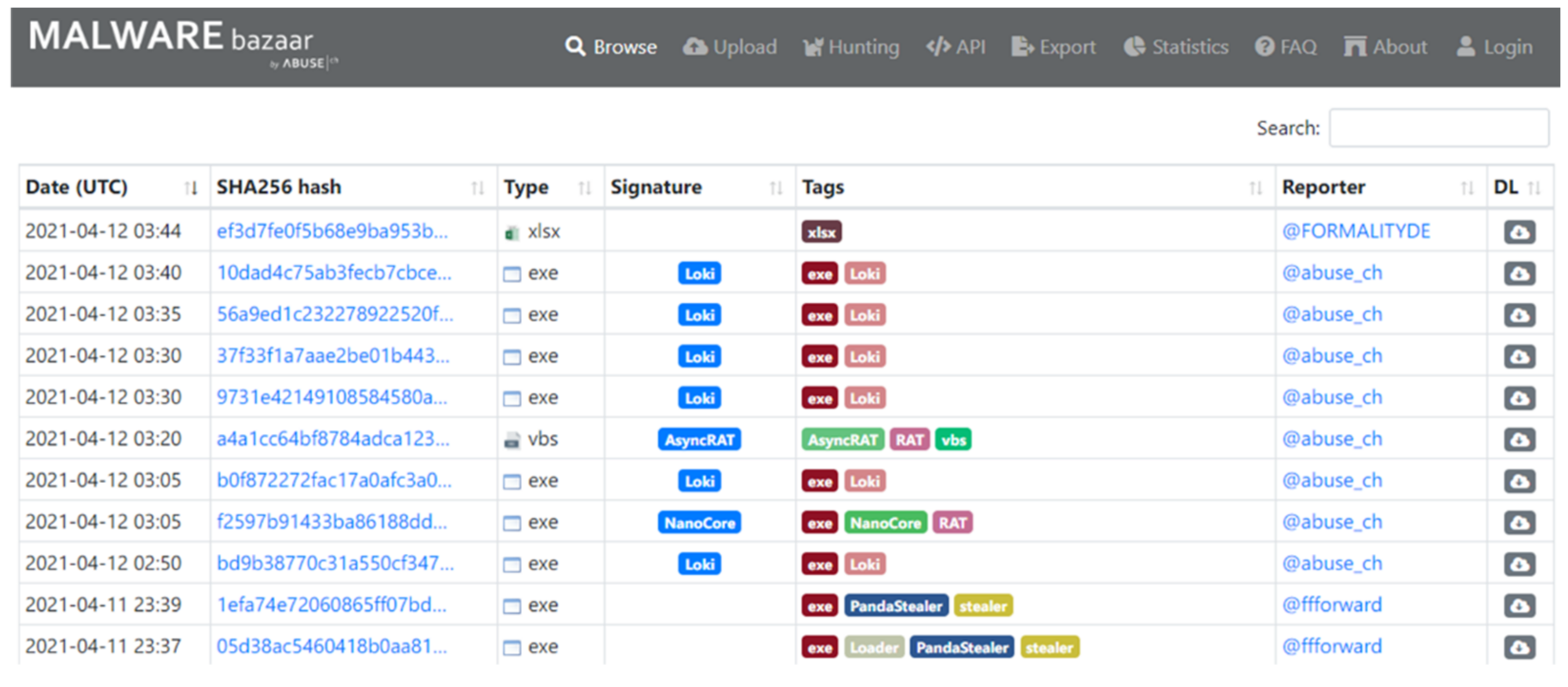
Malware Bazaar is a project of abuse.ch in Switzerland. Its purpose is to share malware samples to help communities resist cyber threats. It saves malware samples that are contributed by the security community and provides the SHA256 hash, file type, and family signature for each. In this work, 10,000 Windows PE samples were downloaded from Malware Bazaar; they comprised 1000 samples in each of ten malware families. Figure 2 presents the sample data.

Additional malware samples were obtained from VirusTotal. The data for the second half of 2020 cover 13,740 PE samples. Since VirusTotal’s sample data do not contain family signatures, these samples are left for use as the corpus for training the Asm2vec model [27].

Malware Bazaar provides the malware family of each sample, but VirusTotal provides each sample without malware family information. Since the purpose of this research is to classify malware, the family of each sample must be known. Therefore, most of the samples that were used in the experiments herein were taken from Malware Bazaar. However, in the data construction in Section 3.2, an Asm2vec model is trained to embed the latent semantics of a binary function into a vector as a feature of each node in the function call graph. The Asm2vec model required only the corpus without the label information. To improve the generalizability of the Asm2vec model, additional samples from VirusTotal are used in this step.

3.2. Dataset Construction

Figure 3 shows the steps of the dataset construction. The first step is to extract the function call graph and function assembly code using Radare2 [31]. Then an Asm2vec model is trained to embed the latent semantics of a binary function into a vector as a feature of each node in the function call graph.

Radare2, also called r2, is a set of libraries and tools for analyzing binary files. Therefore, r2 is used herein to disassemble malware samples to obtain a function call graph. Then, the assembly code for each function is obtained by traversing each function in the graph. The function call graph is thus a directed graph G that comprises a pair G = {V, E}. V is a vertex set that consists of functions V = {v_1, v_2, v_3, …, v_n}, and E is the dependency edge set E = {(x, y)|(x, y) ∈ V²}. Notably, the direction of the dependent edge between functions is determined by the global call graph in r2. Since Windows contains many dynamic-link library (DLL) files, and each DLL file performs many functions, the number of total functions of the Windows DLL is large. For example, user32.dll contains MessageBox, MessageBoxA, MessageBoxW, and other functions. Therefore, all of the functions of a particular DLL file are merged into its DLL file name when transforming into nodes.

The function assembly code that r2 decompiles specifies the function that determines its behavior. Therefore, the Asm2vec model is used to obtain the embedding vector of assembly code as the feature of the function node. Behaviors that are based on the latent semantics of functions can better capture the structure and behavior of samples than those based on the relationship between functions. If only a structural relationship exists between functions, then a misjudgment may be made when they have the same function structure, but they behave extremely differently.

This study uses the open-source tool of asm2vec-pytorch [32] to implement function embedding. Asm2vec is trained using assembly instructions such as an article to learn their latent semantics. The model corpus is established from VirusTotal and Malware Bazaar samples, of which 24,000 are used to generate 800,000 functions as the corpus. Since Windows DLL functions cannot extract assembly code from a sample, the assembly code of the DLL function is replaced by the name of the DLL. Finally, the training model parameters are trained over ten epochs, with 64 training function embedding dimensions, and 128 output function embedding dimensions.

The samples, which have widely varying numbers of function nodes, are converted into graphs. While converting malware samples to graphs, there are some samples that cannot be resolved to function nodes because there are differences in program implementation, or the sample is protected by the packer. The successfully extracted function nodes can further be grouped into two categories. One category is used function node which is called by entry function and export function. The other category is unused function node which does not have entry or export connection to other nodes. Those unused function nodes are pruned from the call graph in the data construction in this study. As shown in Figure 4, the x-axis is the number of function nodes in each sample. The y-axis is the number of the malware sample. The red bars are the count of nodes after trimming, which equals the count of used function nodes in each malware sample. The blue bars are the count of all extracted function nodes in each malware sample, also named full node in the legend, which contains both used function nodes and unused function nodes. The blue bar and red bar at x-axis zero elaborate that the function cannot be extracted from the sample and there is no entry point in that sample, respectively. There are over 2000 samples that cannot be resolved into function nodes which have no full nodes, and over 1000 samples are resolved into over 1000 function nodes, as a result of the use of different programming languages (C/C++, C#, Visual Basic, and others), different compilers (MinGW, MSVC, Borland, and others), and many development frameworks (MFC, .Net Framework, and others). Moreover, the packer protected sample needs to be unpacked first to obtain the correct function structure. Therefore, the call graph is pruned, and functions that are not called by the entry and export functions are excluded. Finally, samples between 10 and 500 are selected as a dataset.

One thousand malware samples for each family were originally corrected. However, in the conversion of samples to graphs, some samples cannot be resolved into function nodes, causing the dataset to contain different numbers of samples of each family.

Table 1. Dataset distribution.

No.	Family	Number of Samples
1	Heodo	775
2	Dridex	749
3	Quakbot	542
4	TrickBot	654
5	AveMariaRAT	286
6	RemcosRAT	330
7	MassLogger	226
8	Gozi	785
9	CobaltStrike	225
10	IcedID	675

presents the distribution of the dataset. The ten malware families are Heodo, Dridex, Quakbot, TrickBot, AveMariaRAT, RemcosRAT, MassLogger, Gozi, CobaltStrike, and IcedID. The total number of samples is 5227.

A training dataset, a validation dataset, and a test dataset that are associated with these samples are used in an experiment. For the investigation of the classification model, 50 samples in each family are selected at random to generate a test dataset and the remaining samples are then split 90% into a training dataset and 10% into a validation dataset. In the experiment on the similarity model, a pair-wise dataset is required, which is generated by the following method. Randomly pair off separately with one same family sample and one different family sample for each sample. The paired dataset has double the original number of samples and is balanced.

3.3. Graph Neural Networks (GNN)

This section introduces the general core concepts on which the GNN model is based [33]. Modern GNN models are based on these core concepts and have various characteristics. Let $G=\left(V,E\right)$ denote a graph with node feature vectors $X_v$ for $v\in V$. $h_r\in \left\{G,V\right\}$ denotes a vector that represents a node or entire graph. GNNs learn a representation vector $h_r$ from the graph structure, and node features $X_v$. $h_v^{\left(k\right)}$ is a representation vector $v$ in the k-th layer; $N\left(v\right)$ are neighboring nodes of $v$, and $u$ are neighboring nodes $\in N\left(v\right)$.

Figure 5 presents the learning strategy of the GNN, which incorporates the aggregate, combine, and readout functions. First, the aggregate and combine functions are used to update the representation vector of the target node by aggregating the representations of its neighbors and combining them with the vector. The updating of the node features reflects graph structures and the relationship between nodes. Similarly, as in the convolution of the CNN, values of neighboring pixels are summed to update a particular pixel. In the graph classification task, the model uses the feature of nodes in the graph to generate a vector that represents the entire graph’s feature. Hence, GNNs apply a readout function that outputs a representation of the whole graph. The readout function aggregates node features from the final layer and is like the flattening and pooling of the CNN. Various GNN models differ primarily in their aggregation schemes. GNNs aggregate the features of collected nodes. GNNs also update a node feature by combining the feature that aggregates from its neighbors with its feature. Accordingly, after the aggregation of k, the representation of each node captures the graph structure and features from its neighbors, and this representation can be used in downstream tasks.

This study uses PyTorch Geometric [34], a geometric deep learning extension library for PyTorch, to construct training models. PyG has implemented many state-of-the-art methods for quickly building GNNs. In the proposed models, first, the GraphSAGE model [35] is used to aggregate and combine the neighborhood features, and then the Set2Set model [36] is used to readout the graph into a fixed size embedding vector.

3.4. Classification Model

First, the classification model uses GraphSAGE, and the aggregate and combine functions for learning the code structural information, as shown in Figure 6 [37]. Second, it uses Set2Set, a readout function that outputs a graph feature, to convert the sample graph into an embedding vector [38]. Then, linear transformations are used to transform the embedding vector into ten dimensions. Finally, the vector is input into to the Softmax function to calculate the distribution of probabilities among malware. GNNs use back-propagate to update model weights based on the prediction error in the learning period to improve the performance. The Softmax function in the classification model is executed in the output layer, predicting the probability that the input sample belongs to each malware family. The family that is associated with the highest probability is ultimately predicted to be the family of the malware.

3.5. Similarity Model

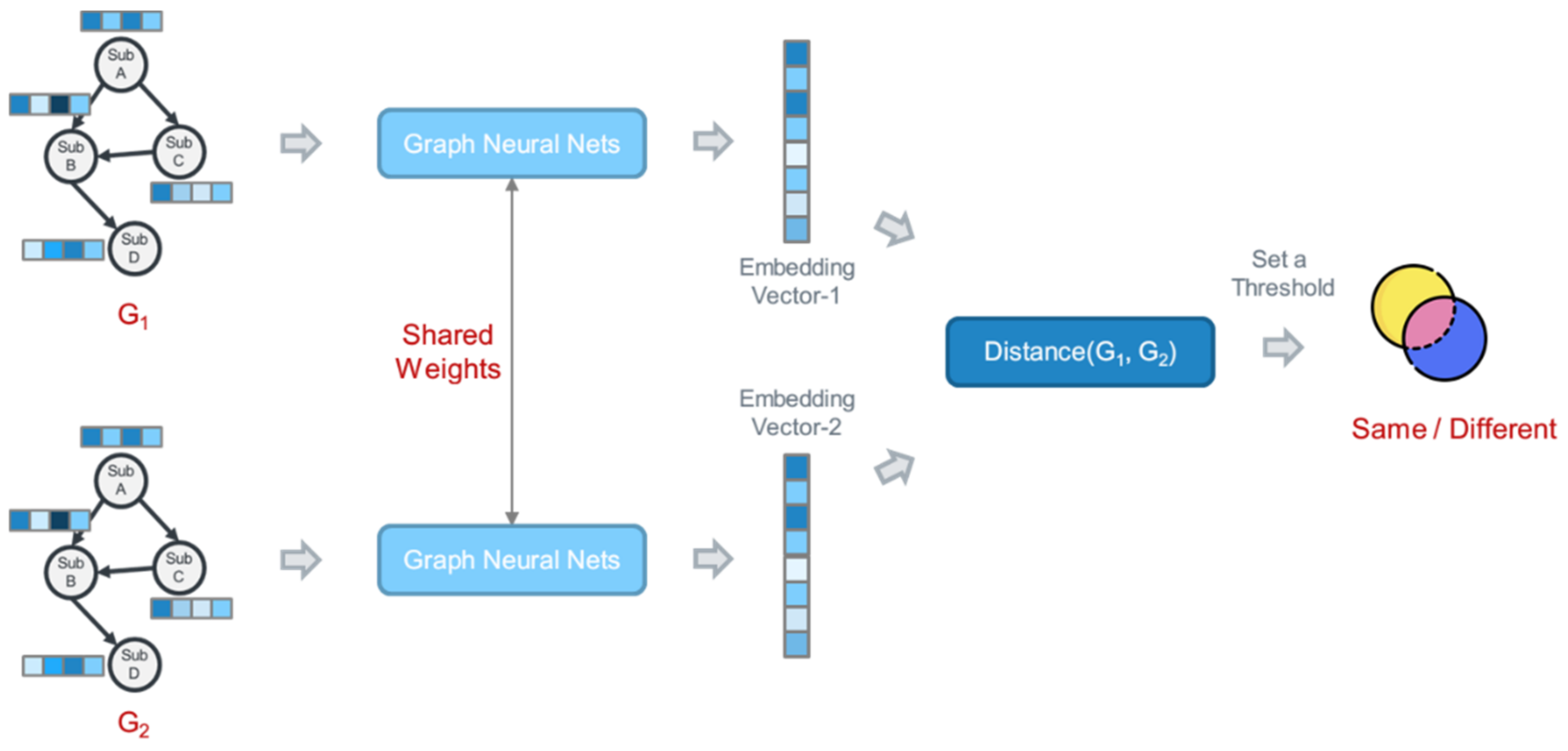
The similarity model is based on the Siamese network, whose inputs are paired and which consists of two graph neural networks with the same parameters and weights. Malware sample pairing firstly involves GraphSAGE to learn the structural information. Secondly, the Set2Set layer calculates the graph feature of the sample graph. Thirdly, the vector is passed into the linear transformation layer and converted into a 32-dimensional vector. Then, the contrastive loss function yields the loss value as the distance between the embedding vectors of two samples [39]. When the two samples are of the same family, a shorter distance between them corresponds to a smaller loss value. When the samples are in different families, a longer distance between them corresponds to a smaller loss value; the loss is zero when the distance exceeds the margin. Finally, the GNN weights are updated using contrastive loss backpropagation to make the model more accurate. Ultimately, after the similarity model training has been completed, the distances between the embedding vectors of the samples can be measured to determine whether the samples are of the same family.

3.5.1. Siamese Networks

The Siamese network refers to a class of neural network architectures that contain numerous unanimous subnetworks. The subnetworks are mirrors of each other, having the same architecture, parameters, and weights. Traditionally, neural networks learn to predict multiple classes, but they must change and be retrained using all available data to change their prediction targets. A Siamese network learns a function that measures the similarity of its inputs by comparing their embedding vectors. Therefore, it can identify whether two inputs are the same or not and face the new class data without being entirely retrained. Figure 7 displays the Siamese network architecture.

The Siamese network usually makes pair-wise learning that does not use cross-entropy loss of learning. The loss function of the Siamese network involves contrastive loss [40], a distance-based loss, rather than a more conventional error prediction loss. This loss is used to learn embedding in the same classes and different classes are far away from each other. Equation (1) defines contrastive loss; Y is zero when the pair are of the same class; otherwise, Y is one. Dw represents the distance between the subnet’s outputs in the Siamese network. The value m is greater than zero’s margin value that distinct classes outside this margin will not contribute to the loss. This means the loss for different classes only exists between zero and the margin.

$$Contrastive Loss=\left(1-Y\right)\frac{1}{2}{\left(Dw\right)}^2+\left(Y\right)\frac{1}{2}{\left\{max\left(0,m-Dw\right)\right\}}^2$$

(1)

Figure 8 presents an example of contrastive loss, in which the colors of the circles represent a class. The class associated with the red circles differs from that of the blue circles. Contrastive loss is high when the blue circles are far from each other or the red circles are close to the blue circles. The loss is low when the blue circles are close to each other or the red circles are far from the blue circles. Therefore, the model depends on the contrastive loss to update its weights by backpropagation, learning how to reduce loss as in the example.

3.5.2. Similarity Model Architecture

This study traverses each sample and randomly selects one sample of the same family and a sample of one other family to form a pair. In conclusion, it generates one same family pair and one different family pair. Therefore, the number of sample pairs is twice the original sample number, and the pairs of the same family and other families each account for half. As shown in Figure 9, the similarity model has two graph neural networks with the same parameters and weights in the Siamese network. Malware sample pairing first uses GraphSAGE to learn the structural information. Secondly, Set2Set calculates the graph feature of the sample graph. Thirdly, the vector is passed into the linear transformation layer and converted into a 32-dimensional vector. Then, the contrastive loss function yields the loss value as the distance between the embedding vectors of two samples. When the two samples are of the same family, a smaller distance between them corresponds to a smaller loss value. When the two samples are of different families, a greater distance between them correspond to a smaller loss value, which is zero when the distance exceeds the margin. Finally, the weights of GNNs are updated using contrastive loss backpropagation to make the model more accurate.

The similarity model is constructed, and the distances between the embedding vectors of the samples can be evaluated to determine whether the samples are of the same family.

Table 2. Parameters of similarity model.

Layer	(Input, Output)	Activation	Remark
GraphSAGE	(128, 64)	Relu	Convolution
GraphSAGE	(64, 64)	Relu	Convolution
GraphSAGE	(64, 64)	Relu	Convolution
Set2Set	(64, 128)		Processing steps = 4
Linear	(128, 64)	Relu
Linear	(64, 32)	Relu	Convolution

presents the parameters of the similarity model in this study. The training learning rate is 10-3, the batch size is 64; the optimization function is Adam; and the Euclidean distance is used to calculate the distance in contrastive loss. Notably, the margin’s condition is set to 1; the distance is 0.5 as the threshold value. Thus, a margin less than or equal to 0.5 belongs to the same family; otherwise, greater than 0.5 belongs to different families.

4. Performance Analysis

Performance analyses using the classification and similarity models are discussed and analyzed. The performance of the similarity model is evaluated by visualizing embedding vectors as an image, and it is compared with previously developed models.

This study introduced the early stopping mechanism during the training process, which can avoid over-fitting of the model. It tracks the validation loss of each epoch, and training stops if the loss stops decreasing for several consecutive epochs. At the same time, the checkpoint of the model will be saved every time when validation loss is a new low.

4.1. Classification Model

The prediction result is drawn as a confusion matrix and measures the performance using evaluation metrics. These evaluation metrics are used to measure the performance of binary classification tasks. However, the classification model performs a multi-classification task, the macro average of the classification model for each class is calculated. In addition, the receiver operating characteristic (ROC) curve is drawn separately for each class and calculates the area under the ROC curve. Finally, the macro-AUC is also one of the comprehensive evaluation metrics of the classification model. The indicators mentioned before are shown in Figure 10 and

Table 3. Performance of classification model.

Accuracy	Precision	Recall	F1-Score	AUC
0.934	0.938	0.934	0.935	0.963

. The classification model has a macro accuracy and macro recall of 0.934, a macro precision of 0.938, a macro f1-score of 0.935, and a macro-AUC of 0.997 on a test dataset.

4.2. Similarity Model

The similarity model predicts whether the pair-wise data is in the same family and thus it is unnecessary to calculate the average of metrics. Figure 11 and

Table 4. Performance of similarity model.

Accuracy	Precision	Recall	F1-Score	AUC
0.920	0.929	0.910	0.919	0.920

show the performance result of the similarity model using a confusion matrix, an ROC curve, and evaluation metrics. The similarity model has an accuracy of 0.92, a precision of 0.929, a recall of 0.91, a f1-score is 0.919 and an AUC of 0.92 on a test dataset.

A Siamese network uses contrastive loss to cluster data in the same class and keeps data in distinct classes far from each other. Hence, samples are mapped into vector space using the similarity model, and principal component analysis (PCA) is used to reduce the dimensionality of the embedding vector of the samples. Each sample is transformed into a 32-dimensional vector by the model. This 32-dimensional vector is mapped to a two-dimensional space using PCA, and a scatterplot is generated, as shown in Figure 12. The ten families of samples are clustered by family and distributed among various locations. Accordingly, the similarity model has effectively learned the relationships between samples.

4.3. Performance Comparison

The ssdeep and TLSH techniques are based on fuzzy hash algorithms, and they are widely used to identify malware. Consequently, fuzzy hash algorithms are compared and used to generate a baseline. If the similarity score output by ssdeep is greater than zero, then the malware pair are in the same family; else, they are in different families. The threshold of the TLSH is set to 100, as recommended in Reference [39]. The malware pair are in different families when the distance score of the TLSH exceeds 100; otherwise, the pair are in the same family.

Although ssdeep and TLSH are mainly used for comparing the similarity, they can also perform the classification function by transforming samples into related hash values and mapping to related categories. First, the sample is transformed into hash values. Then, the hash values are mapped with the training dataset. When the sample is similar to a specific category in the training dataset, the input sample can be classified as that category. Therefore,

Table 5. Classification model performance comparison with previous works.

Technique	Test Dataset (Accuracy)	Test Dataset (Precision)
Ssdeep [6]	0.627	0.572
TLSH [7]	0.634	0.593
Proposed method	0.934	0.938

compares the performance of the classification model with ssdeep and TLSH. From the experimental result, the method proposed by this study is higher than traditional fuzzy hash methods. This is because fuzzy hash methods transform whole files into hashes, while the graph classification method caches the relationship between the executed functions.

Reference [25] proposed the MSM_GCN strategy, based on a study of similarity matching of malware families based on a graph similarity metric using graph convolutional networks. However, they did not provide sufficient experimental details concerning, for example, data pre-processing and model hyper-parameters. Therefore, the MSM_GCN that is used for comparison is consistent with the original concept but may have been differently implemented. Herein, a fixed feature value of one is added to each node and the graph feature is obtained from global_max_pool.

Table 6. Similarity model performance comparison with previous works.

Technique	Test Dataset (Accuracy)	Test Dataset (Precision)	Unseen Dataset (Accuracy)	Unseen Dataset (Precision)
Ssdeep [6]	0.605	0.559	0.519	0.510
TLSH [7]	0.619	0.568	0.541	0.522
MSM_GCN [25]	0.764	0.776	0.547	0.560
Proposed method	0.920	0.929	0.704	0.695

compares the performances of the similarity model herein with the ssdeep, TLSH, and MSM_GCN techniques. With respect to the similarity among malware families, finding variants that belong to the same family is costlier than finding those that belong to different families. Hence, the precision is more important than the recall in this study. The widely used fuzzy hash method takes the raw malware sample as input, which does not contain the relation of function call graph and therefore has lower precision compared with graph methods. The precision of the proposed method is 0.196 higher than that of MSM_GCN technique, and the proposed method performs best among the four compared methods. The families in the test dataset are considered during model training. Therefore, an unseen dataset is used herein to test the effectiveness of family verification; it contains three new families and 500 samples that did not appear in the training dataset d. The function call relationship and the function assembly content are obtained by analyzing the malware to generate a graph that represents its functional structure during the model training period. The proposed model’s overall performance decreases by about 0.2 when tested on the unseen dataset, similar to the MSM_GCN technique. Even when the model predicts a malware family that has never been seen before, it can still verify around 70% of the malware families in the unseen dataset. Hence, the similarity model has better performance and scalability than the classification model with unseen data.

From the performance results in Table 5, although the performance on unseen dataset can reach 70%, it is still lower than the performance on the test dataset. Therefore, prediction using the similarity model with the unseen dataset is visualized using PCA to observe the embedding performance on an unseen dataset. There are three families, NanoCore, Loki, and njrat in the unseen dataset. As shown in Figure 13, NanoCore and Loki have grouped as clusters and hence the similarity model can determine whether various pieces of malware are similar using graph data structures. However, some samples of njrat and Loki are close to each other. The results reveal that the similarity model easily misidentifies the two families of Loki and njrat.

5. Conclusions

This work proposes a novel method for identifying malware families that is based on GNNs. The behavior of malware is represented by a graph data structure that is based on the call relationship and the potential semantics of the malware function. GNNs are used to aggregate the nodes on the graph and update the feature of specified nodes. Then, the readout function is used to output a fixed-size graph-level embedding. In this work, a similarity model that is based on Siamese networks is implemented to measure the distance between two samples in the feature space, and thus to determine whether they belong to the same class. Finally, the proposed similarity model was tested using an unseen dataset and a test dataset from Malware Bazaar. The accuracies of the model with a test dataset and an unseen dataset were 0.920 and 0.704, respectively. The similarity model outperformed previously developed techniques.

This study has three goals worthy of further research and improvement in the future. First, add more sample data. More malware families can be collected, and benign software can also be added to the dataset to make the model more versatile. Second, work on anti-obfuscate research. Some malware interferes with the analysis by adding packs and obfuscations which make the decompiler unable to parse the function call graph and assembly code content correctly. The third is to improve the method of transforming malware into a graph. Improve the processing of DLL functions and study how to find the key functions and ignore the general functions generated by the compiler.