Abstract
Supervised image denoising methods based on deep neural networks require a large amount of noisy-clean or noisy image pairs for network training. Thus, their performance drops drastically when the given noisy image is significantly different from the training data. Recently, several unsupervised learning models have been proposed to reduce the dependence on training data. Although unsupervised methods only require noisy images for learning, their denoising effect is relatively weak compared with supervised methods. This paper proposes a two-stage unsupervised deep learning framework based on deep image prior (DIP) to enhance the image denoising performance. First, a two-target DIP learning strategy is proposed to impose a learning restriction on the DIP optimization process. A cleaner preliminary image, together with the given noisy image, was used as the learning target of the two-target DIP learning process. We then demonstrate that adding an extra learning target with better image quality in the DIP learning process is capable of constraining the search space of the optimization process and improving the denoising performance. Furthermore, we observe that given the same network input and the same learning target, the DIP optimization process cannot generate the same denoised images. This indicates that the denoised results are uncertain, although they are similar in image quality and are complemented by local details. To utilize the uncertainty of the DIP, we employ a supervised denoising method to preprocess the given noisy image and propose an up- and down-sampling strategy to produce multiple sampled instances of the preprocessed image. These sampled instances were then fed into multiple two-target DIP learning processes to generate multiple denoised instances with different image details. Finally, we propose an unsupervised fusion network that fuses multiple denoised instances into one denoised image to further improve the denoising effect. We evaluated the proposed method through extensive experiments, including grayscale image denoising, color image denoising, and real-world image denoising. The experimental results demonstrate that the proposed framework outperforms unsupervised methods in all cases, and the denoising performance of the framework is close to or superior to that of supervised denoising methods for synthetic noisy image denoising and significantly outperforms supervised denoising methods for real-world image denoising. In summary, the proposed method is essentially a hybrid method that combines both supervised and unsupervised learning to improve denoising performance. Adopting a supervised method to generate preprocessed denoised images can utilize the external prior and help constrict the search space of the DIP, whereas using an unsupervised method to produce intermediate denoised instances can utilize the internal prior and provide adaptability to various noisy images of a real scene.
1. Introduction
Image denoising is an essential issue in the field of image processing that aims to recover a clean image from a noisy image. A noisy image is generally formulated as follows:
where y is the observed noisy image, x is the corresponding clean image for recovery, and n is the additive noise. Here, n is typically assumed to satisfy the zero-mean normal Gaussian distribution, where the standard deviation reflects the level of image interference by noise.
While traditional image denoising models (e.g., BM3D [1], NLM [2], and WNNM [3]) have achieved state-of-the-art peak signal-to-noise ratio (PSNR) performance, deep neural network (DNN)-based methods have achieved great success. In the past few years, DNN-based image denoising methods have shown a strong capability to learn natural image priors from a large number of example images, thereby significantly improving the denoising effect. Numerous DNN-based image denoisers have been proposed, such as DnCNN [4], FFDNet [5], GANID [6], and CBDNet [7]. In DnCNN [4], Zhang et al. introduced batch normalization and residual learning to enhance the network training performance and speed up the training process. DnCNN achieved superior performance compared with traditional non-learning-based methods for additive white Gaussian noise (AWGN) removal. Subsequently, numerous modified representative neural networks have been proposed for image denoising, such as U-Net [8], non-local networks [9], and wavelet transform networks [10]. FFDNet provides a flexible solution for dealing with spatially variant noise and AWGN with different noise levels. FFDNet uses both the noisy image and its tunable noise level map as the network input and achieves satisfactory results on both synthetic and real noisy images. Although the denoising performance of the aforementioned methods is significantly improved compared with non-learning-based methods [1,2,3], they generally suffer from the limitation of convolution operations. Convolution kernels cannot flexibly adapt to different image contents because of their static filter weights, and the convolution operator has a small receptive field, which limits its applicability to long-range dependency modeling. Therefore, transformer-based denoising models have been proposed to mitigate the shortcomings of DNN-based methods [11,12]. SwinIR [11] employs a convolution layer to extract shallow features and a stack of residual Swin transformer blocks to extract deep features. Restormer [12] is also a transformer-based image restoration method that can process high-resolution images and model the global context using self-attention across channels instead of the spatial dimension to alleviate the computational bottleneck. The supervised learning studies mentioned above [4,5,11,12] have improved the image denoising performance to some extent. However, these denoisers critically depend on the quantity and diversity of noisy-clean image pairs, which are extremely difficult and expensive to collect in real-world scenarios. For example, collecting high-quality noiseless images as training datasets is essential for medical image processing. However, high-quality labels are often derived from long scan durations and high doses, which are limited in clinical practice. Moreover, most supervised DNN methods learn the denoising model using abundant training data and only lead to promising denoising performance on specific datasets. The performance of these denoisers drops dramatically once the unseen noisy images are reconstructed.
Compared with supervised methods, unsupervised learning is much more valuable for many real-world applications where no ground-truth image is available [13,14]. Recently, several unsupervised [15,16,17,18,19,20,21,22,23] approaches have been proposed to eliminate the dependence on clean images. Rather than using noisy-clean pairs for training, the Noise2Noise method [15] uses multiple noisy images of the same scene to train a denoising DNN. Its performance is close to that of DNNs trained on noisy-clean pairs. Subsequently, Noise2Void [16] and Noise2Self [17] were proposed to train DNNs using only unorganized noisy image pairs. To avoid learning identity mapping, the blind-spot networks proposed in Noise2Void only utilize the neighboring pixels to predict each pixel. Similar strategies were used in the parallel work of Noise2Self. Although Noise2Noise, Noise2Void, and Noise2Self achieved good denoising results, the noisy images used for model training were heavily correlated to the observed noisy image. Collecting such noisy images is also challenging and costly in practice. Unlike blind-spot methods, the training pairs used in Noisier2Noise [18] and Noisy-as-Clean [19] are generated by adding synthetic noise to the observed noisy image. However, it is difficult to specify a noise-generating model for real-world scenarios. Similar to Noiser2Noise and Noisy-as-Clean, R2R [20] corrupts noisy images with specific noise levels to generate training pairs. However, prior knowledge of the noise levels required in R2R is difficult to collect in real-world scenarios. Another method, Self2Self [21], proposed a dropout denoiser that was trained on Bernoulli sampled noisy image pairs. Self2Self generates multiple recovered images and uses the average of the recovered images as the final reconstructed result. This method has achieved better performance in real-world image denoising; however, it still cannot handle low-illumination images. To improve denoising performance, Neighbor2Neighbor [22] constructs a noisy pair by subsampling a given noisy image. However, its performance still relies heavily on a large-scale training dataset to a great extent.
In contrast to the aforementioned unsupervised image-denoising methods, deep image prior (DIP) [23] has received much attention. DIP adopts a generator network to capture low-level image statistics prior without the need for pretraining or additional data. The network parameters were optimized by considering the given noisy image as the learning target with a random noise input. Although the DIP demonstrated that the trained DNN can represent a well-recovered image, its performance is relatively weak compared with state-of-the-art supervised methods, especially for synthetic image denoising. The main reason for this is that the image quality of the DIP learning target is relatively low, which leads to a large search space and slow convergence. Moreover, the two DIP learning methods cannot generate identical denoised images even given the same network input and the same targeting noisy image due to the randomly initialized network weights. For different noisy images, the reconstruction processes lead to more diverse recovery results.
In this study, aiming at improving the denoising performance of DIP, we propose a two-stage unsupervised image denoising framework that achieves better performance than state-of-the-art supervised models. In contrast to DIP, which generates only one denoised image, we try to reconstruct a set of intermediate denoised images across the image space using multiple DIP learning processes and take the fusion of the intermediate images as the final denoised image. In our study, we first propose a two-target DIP learning strategy to improve the denoising effect. A preliminary image, together with the given denoised image, is taken as a DIP learning target. Through the proposed up- and down-sampling strategy, multiple sampled images of a denoised image, which is generated by a supervised denoising method, can be obtained. These preliminary images were learned by several two-target DIP optimization processes to generate multiple intermediate denoised instances. The intermediate denoised images, which contain different recovered details, are complementary. To further improve the denoising effect, we developed an unsupervised image fusion network to generate weight maps for the intermediate denoised instances, which we used to fuse the DIP-recovered instances into a single denoised image. We show that superior denoising results can be achieved using our method compared to the standard DIP method and state-of-the-art supervised image denoising methods.
2. Related Work
The image denoising problem can often be represented as an energy minimization problem of
where y is a given noisy image, is used to compare the generated image to y, and is a regularizer. In [23], Ulyanov et al. proposed a randomly initialized DNN called DIP to solve image-denoising problems. In the DIP framework, the optimization problem is expressed as follows:
where f denotes the DNN model, is the random initialized network parameter, z denotes the random noise input of the network, is the learned network parameter, and is the result of the recovery process. Given a noisy image y, the DIP learning process attempts to find the proper value of that can reproduce the noisy image. It has been demonstrated that a DIP network contains prior knowledge, such as the low-level structure of natural images. It can remove noise from corrupted images with a certain number of iterations. However, the denoising performance of DIP is not as satisfactory as that of state-of-the-art methods; that is, a single run leads to a far lower PSNR value than state-of-the-art methods, such as BM3D [1], especially for synthetic noisy image denoising. This is because the DIP optimization process can be considered a process of finding the best-quality instance in the image space. The distance between the low-quality target image and the clean image was larger than that between the high-quality target image and the clean image. Figure 1 shows the variation in the PSNR values of the two denoised images generated from the DIP optimization processes versus the number of training iterations. The two DIP optimization processes used two different images as learning targets. One is a preliminary image, and the other is a noisy image. The preliminary image was a denoised image generated using a pre-trained supervised image denoising method. As shown in Figure 1, DIP achieves a PSNR of 28.93 dB after 3083 iteration steps when using the preliminary image or the noisy image as the learning target. The PSNR is increased to 30.16 dB in iteration 8999 when using the preliminary image as the learning target; however, the PSNR decreases to 23.59 dB in iteration 8999 when using the noisy image as the learning target. This implies that the denoised image generated from the DIP gradually converges to the target image as the number of iterations increases. Therefore, using images with better quality as the DIP learning target can avoid overfitting and help achieve a better denoising result.
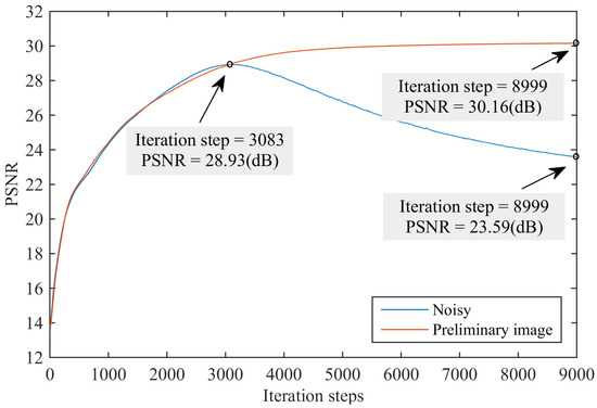
Figure 1.
Learning curves for the reconstruction task using natural and noise images. PSNR of a natural looking image is higher compared to that of the noise image.
DIP shows that the unsupervised DNN is capable of capturing low-level image statistics. However, given the same network input and learning target, DIP cannot generate identical denoised images owing to the randomly initialized network weights. To illustrate its uncertainty, we compared two denoised images generated from the DIP optimization processes. Figure 2 shows the variations in mean square error (MSE) between the network outputs of the two DIP optimization processes as the number of DIP iterations increases. In the two DIP learning procedures, we used the same noisy image as the learning target and the same random noisy image as the input. We can see from Figure 2 that MSEs show a downward trend before 4000 iterations, whereas MSEs remain to after 4000 iterations. It is apparent that different DIP optimization processes generate different denoising results. It is impossible to obtain the same network output at the same iteration steps, even when given the same network input z and the same learning target. To investigate the detailed difference between the denoised images generated from different DIP learning processes, we conducted experiments on noisy images, as shown in Figure 3. The PSNR of the two instances generated from DIP is 27.40 and 27.43 dB, respectively. Although the PSNR of the two denoised instances is similar, the contents of these instances are different. To measure the reconstruction error (RE) r, we calculated the difference between the denoised instance and clean image c with respect to the pixel
where and are the pixel indices, W and H are the width and height of the denoised instance, respectively, and T is the threshold for visualization.
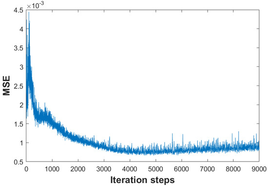
Figure 2.
Variations in the MSE between the network outputs obtained from two DIP optimization processes along iteration steps.
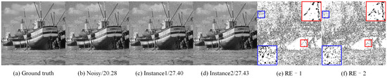
Figure 3.
Visual comparison of the denoised instances generated from two different DIP optimization processes. The quantitative PSNR results are listed behind the noisy image and two instances.
Figure 3 shows a visual comparison of two denoised instances generated from two DIP optimization processes with the same network input and the same target noisy image. As shown in Figure 3c,d, the two denoised instances are similar. However, from Figure 3e,f, there are evident differences between the two denoised instances. In Figure 3e,f, we also zoom in on two regions for a better view. Clearly, the blue rectangle of RE–1 contains more black points () than that in the blue rectangle of RE–2, whereas the black points in the red rectangle of RE–1 are fewer than those in RE–2. The black points indicate that the pixel at this point in the denoised instance has the same or similar intensity as the pixel at the corresponding position in the clean image. We can conclude that the denoised images generated from the different DIP learning processes are complementary to each other.
3. Methodology
To utilize the diversity and complementation of denoised images generated from DIP to obtain better denoising results, we propose certain preprocessing strategies to generate a set of intermediate denoised instances of the noisy image and then fuse them into the final denoised image. An overall flowchart of the proposed method is shown in Figure 4. As shown in Figure 4, the proposed method comprises two main steps. In the first step, we propose a two-target DIP learning strategy to produce an intermediate denoised image, . Specifically, we first used the given noisy image and preliminary image as the learning targets of the DIP network. Using two targets in DIP learning can constrict the image search space and improve the denoised result. Then, we repeat the two-target DIP optimization process n times with different network inputs and different preliminary images to generate n intermediate denoised images . To generate the preliminary images, the given corrupted image y is fed into a pre-trained denoising model, such as FFDNet, to generate a cleaner image p. Then, we employ an up- and down-sampling strategy to generate diverse sampled images of p. In the second step, we develop an unsupervised image fusion network to fuse intermediate denoised images with a single denoised image . These intermediate denoised images, which have similar image quality and different local details, complement each other. Fusing these into a denoised image can further improve the denoising effect.
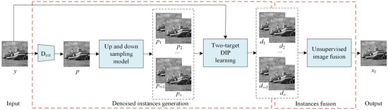
Figure 4.
The overall flowchart of the proposed method.
3.1. Preliminary Images Generation
According to the analysis in Section 2, it is important to collect a set of cleaner images such that the denoised instances obtained from the DIP can have diverse reconstruction effects. To this end, we first adopt a pre-trained state-of-the-art image denoising method, FFDNet, to reconstruct the given corrupted image y. FFDNet is one of the best DNN-based denoising models and has obtained remarkable denoising results for real-time noisy images. Clearly, reconstructed image p generated by FFDNet has a higher image quality than y, and using p as the learning target of DIP can achieve a much better denoising effect. However, in the proposed method, we use only p to produce more diverse, cleaner instances. We develop an up- and down-sampling strategy to obtain diverse instances of p. Specifically, we first employ the up-sampling method proposed by [24] to obtain a super-resolution version of p, denoted by . The up-sampler can reshape the input image of size into . Where H and W are the image height and width, respectively, and C denotes the number of channels, that is, for the color image and for the grayscale image. Then, we adopted a randomly selected down-sampler to generate multiple down-sampled instances of . The details of using a randomly selected down-sampler to generate a set of down-sampled images from image are as follows. First, image is divided into cells with size . Here . Subsequently, one location is randomly selected in the -th cell n times. The points corresponding to n locations are taken as the -th point of the down-sampler . For all cells, the random location selection is repeated, n down-sampled images of size are derived. We provide a visual example of generating instances with a randomly selected down-sampler in Figure 5. In Figure 5, image contains pixels and is divided into cells. For each cell, one point was randomly selected to generate a down-sampled image. For example, we select point “26” in the (1,3)-th cell and point "66" in the (3,3)-th cell as the (1,3)-th pixel and the (3,3)-th pixel of down-sampled image 1, respectively. The randomly selected down-sampled process was repeated six times, and six down-sampled images were obtained.
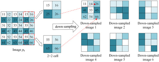
Figure 5.
Example of the down-sampling images with the randomly selected down-sampled generator.
3.2. Two-Target DIP Learning
In Section 3.1, we obtained multiple preliminary images from the given noisy image to generate recovered intermediate images. In this section, we introduce our unsupervised training scheme that uses these preliminary images. Our method uses different random noise image as the network input and uses both the given noisy image and preliminary image as learning targets. As discussed in Section 2, using a cleaner preliminary image as the DIP learning target can restrict the DIP searching space and improve the denoising effect. However, much useful information is still contained in the given noisy image. To further improve the denoising effect, we propose a two-target DIP learning strategy that uses both the given noisy image and the preliminary image as learning targets to generate intermediate denoising images. Figure 6 shows the framework of two-target DIP learning.
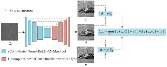
Figure 6.
Framework of the intermediated denoising image generation.
The unsupervised two-target denoising model can be described as
where y denotes the given noisy image, is the preliminary image generated by the cleaner intermediate image-generation approach, and . The loss function is defined as follows:
where the term measures the MSE between the generated image and given noisy image y
and the term measures the MSE between the generated image and intermediate image
The loss function was used to constrain the range of DIP output. Using can effectively prevent overfitting and improve the reconstruction results. We conduct the ablation experiments to demonstrate the effectiveness of the two-target DIP learning strategy and describe the experimental results in Section 4.2.
3.3. Unsupervised Image Fusion
Given a set of intermediate denoising images , the final denoised image for the pixel positioned at () is computed as a weighted average of pixels in the same position in denoised instances
where the weight map is generated from the proposed unsupervised fusion network, and k is the index of the denoised instances, . The family of weights satisfies conditions and . Figure 7 shows the weighted fusion scheme of the intermediate denoising images. The fusion network has a symmetric encoder–decoder architecture with skip connections. We denote as n feature maps from a single image. We first concatenate along the channel axis as , and then D is taken as the learning target of the fusion network. The output of the fusion network contains n channels, and the feature map of each channel is used as the weight map of .
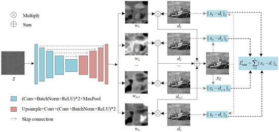
Figure 7.
Unsupervised intermediate denoising images fusion network.
The fusion network is learned in an unsupervised manner, and the loss function measures the sum of the MSEs between the fusion image and each intermediate denoised instance
In Equation (10), to minimize the loss , the sum of the differences between pixels in and the pixels of the corresponding position in the intermediate denoised images should be the smallest. This means that the fusion image preserves the common details in the intermediate denoised images so that it can achieve a better image quality.
4. Experiments
4.1. Experimental Setting
In this section, we demonstrate the denoising performance of our proposed method by comparing it with state-of-the-art methods, such as BM3D [1], WNNM [3], DnCNN [4], FFDNet [5], DAGL [25], DeamNet [26], DRUNet [27], IRCNN [28], DIP [23], N2V [16], and SwinIR [11]. Three datasets were utilized for the performance comparison: Set5 [29], Set12 [4], and BSD68 [30]. The Set12 dataset consists of 12 grayscale images that are widely used for image denoising tests. The BSD68 dataset contains 68 grayscale images randomly selected from the BSD500 dataset. The Set5 dataset comprises traditionally used color images for comparing image denoising methods. The images in the three databases are corrupted by AWGN with noise levels . We used PSNR as an evaluation metric. A better method is expected to yield a higher PSNR value.
4.2. Ablation Experiments
In the proposed method, we employed a two-target DIP learning strategy to generate intermediate denoising images. To compare the performance of different images as learning targets, we conducted ablation experiments on the Set12 dataset. Table 1 lists the average PSNR results for Set12. In Table 1, the columns “Noisy” and “”, correspond to the results of using the given noisy image and a single preliminary image as the learning target, respectively. Column “Noisy+” indicates the use of the proposed two-target learning strategy. It is clear that simply using a preliminary image as the DIP learning target can improve the PSNR. Moreover, the use of a two-target learning strategy can further improve denoising performance. Compared with the PSNR result of using noisy images as the DIP learning target, the PSNR result of the two-target DIP learning method was significantly improved (more than 1.6 dB). The reason behind this is because the preliminary image, which has a higher image quality than that of the given corrupted image, is generated from a supervised image denoising method. Some pixels in the preliminary image are inevitably over-smoothed. Meanwhile, the corresponding pixels in the noisy image may be clean pixels that can be used as complementary information to the preliminary image. Therefore, using both preliminary and noisy images can provide more useful information for image denoising.

Table 1.
The PSNR (dB) performance of the Set12 dataset while taking different images as the learning target of the DIP optimization process.
During the intermediate image fusion process, the number of instances used for image fusion is an important factor. To explore the impact of the instance numbers on the denoising results, ablation experiments were performed on Set12 with noise level . Table 2 shows the average PSNR using two to eight intermediate instances for image fusion on Set12. As presented in Table 2, using eight instances achieves the highest PSNR value, whereas using four instances can reach a PSNR value above 31 dB. Considering that generating four instances is much more efficient, and the PSNR result of using four instances is only 0.09 dB lower than that of using eight instances, we finally used four instances to generate a denoised image.
Table 2.
Averaged PSNR (dB) of the Set12 dataset while using different numbers of intermediate instances for image fusion.
4.3. Gray Image Denoising
The averaged PSNR results of the different metrics on the Set12 and BSD68 datasets are reported in Table 3, and the best three performances are highlighted in boldface. Table 4 also reports the PSNR values of the different methods for 12 Gy images in the Set12 dataset, and the best two performances are highlighted in bold font. Evidently, the proposed method shows a good performance on two datasets with three noise levels. Specifically, the proposed method has an average PSNR gain of approximately 1 dB over BM3D on both Set12 and BSD68 datasets. It also surpasses the DnCNN and the FFDNet by an average PSNR of 0.5 dB on the Set12 dataset and 0.25 dB on the BSD68 dataset. Compared with unsupervised methods DIP and N2V, the PSNR performance of the proposed method is about 2 dB higher than that of DIP and N2V. This is because DIP and N2V utilize only the internal prior, whereas the proposed method can learn both the internal and external priors. Moreover, the proposed method can utilize the uncertainty of the DIP to obtain multiple denoised instances that are complementary to each other so that the fused image can have a better denoising effect.
Table 3.
Comparison of the averaged PSNR (dB) of different methods on the Set12 and BSD68 datasets. The best three performances are highlighted in boldface.
Table 4.
PSNR (dB) values of different methods on 12 gray images in the Set12 dataset with noise level at 15, 25, and 50. The best two performances are highlighted in boldface.
As presented in Table 3, compared with the newly proposed supervised method SwinIR, our method outperforms SwinIR with noise levels of 15 and 25 on both the Set12 and BSD68 datasets. These results indicate that our method can handle more complex corrupted images and achieve better performance than the existing models. It can be seen from Table 3 and Table 4 that the proposed method achieves relatively low performance on “Barbara”, which makes the average PSNR with noise level 50 of the proposed method lower than that of DAGL, DeamNet, DRUNet, and SwinIR. A possible reason is that DIP-based methods are not good at learning non-local self-similarity prior when images at high noise levels contain rich textures and repetitive structures. One possible solution to this problem is to improve the quality of the preliminary image. As discussed in Section 2, the image quality of the DIP learning target can constrict the search space. Using a learning target with better quality can avoid overfitting and help achieve a better denoising result. In the proposed method, FFDNet is first employed to preprocess the given noisy image, after which the two-target DIP and unsupervised fusion network are employed to generate the final denoised image. If other supervised denoisers with better denoising performance, such as DRUNet and SwinIR, are utilized to preprocess the given noisy image, the final denoising performance can be further improved.
In Table 3, we also compare the performance of two methods proposed in our previous works [31,32]. In [31], we first employed a set of state-of-the-art image denoisers to preprocess the given noisy image and obtain multiple intermediate denoised images. These intermediate denoised images were then concatenated and fed into an unsupervised deep fusion network to generate the final denoised image. In [32], we utilized two state-of-the-art denoisers to generate the preliminary denoised images and proposed an unsupervised fusion network to fuse the two preliminary denoised images into the final denoised image. As shown in Table 3, the performance of the proposed method is slightly lower than that of our previous methods. The main reason for this is that the proposed method employs only FFDNet to generate multiple intermediate denoised images. The diversity of the intermediate denoised images is not as high as that of the intermediate denoised images generated in our previous studies. The two methods we previously proposed achieved very good performance on synthetic noisy image denoising. However, it should be noted that the denoiser proposed in [32] did not improve the performance of real-world noisy images, and the method proposed in [31] cannot be used for real-world image denoising.
4.4. Color Image Denoising
To test our proposed method on color image denoising, we conducted experiments on the Set5 dataset and compared its denoising results with those of the DIP, FFDNet, VDNet [33], SwinIR, CBM3D, DRUNet, DnCNN, and N2V methods. Table 5 reports the color image denoising performance of different methods with noise levels on the Set5 dataset. The three best methods are highlighted in bold font. One can observe that the proposed method significantly outperforms the unsupervised methods DIP and N2V and achieves a higher PSNR than most of the supervised methods.
Table 5.
Comparison of the averaged PSNR (dB) of different methods on the Set5 dataset. The best three performances are highlighted in boldface.
4.5. Visual Comparison
To provide a direct visual comparison of the denoised images, Figure 8 shows the ground truth of a grey image, its noisy image (), and denoised images generated using different methods: BM3D [1], WNNM [3], DnCNN [4], DRUNet [27], DIP [23], FFDNet [5], SwinIR [11], N2V [16], and the proposed method. As shown in Figure 8, our proposed method achieves the best PSNR value on the "Couple" image. By observing the enlarged areas of the recovered images generated by different competing methods, we can see that the denoised images generated by FFDNet, DRUNet, and SwinIR lost some edge information and over-smoothed the image, whereas our proposed method preserved more image details. Visual images of denoising results can be found at https://github.com/chenxiaojun0101/Learning-from-multiple-instances-for-Image-denoising (accessed on 10 September 2022).
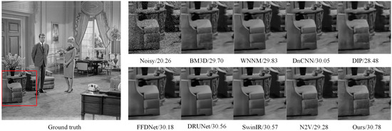
Figure 8.
Visual comparison of our proposed method against the competing methods with the quantitative PSNR results listed behind the noisy and denoised images.
Figure 9 shows the color image denoising results of different methods with a noise level . Compared with grayscale images, color images contain more complex texture details, which is conducive to testing the robustness of denoising methods. As shown in Figure 9, the structural information and texture details in the ground truth are well preserved in the denoised image generated by the proposed method. The PSNR result of our proposed method is significantly higher than that of DIP and N2V and is very close to that of the newly proposed supervised SwinIR method. This indicates that our proposed method can effectively recover the noisy image while preserving the image details to the extent possible.
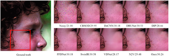
Figure 9.
Visual comparison of the denoised results on the color image dataset. The quantitative PSNR results are listed behind the noisy and denoised images.
4.6. Real-Image Denoising
In real-world applications, the distribution of real noise is often unknown. Therefore, the performance of state-of-the-art denoising methods degrades sharply when denoising noisy real-world images. To further demonstrate the effectiveness of our proposed method, we tested it on real-world noisy images and compared its denoised results with those of CBM3D [1], LIME [34], FFDNet, Restormer [12], VDNet [33], Yu2022 [32], and DIP. Figure 10 shows one low-light image from the SCIE [35] dataset and its denoised versions generated using different methods. As shown in Figure 10, most denoising methods enhance low-light images with a large amount of noise remaining at the edge of the text. However, the proposed method can preserve the texture details of the edge while removing noise. In Figure 11, we compare the denoised results of a RAW camera image from the Nam [36] dataset. Clearly, the PSNR of the proposed method is 3.41 dB higher than that of the DIP method. Compared with VDNet, which was developed for real-world noisy image denoising, our proposed method achieves a 2.83 gain over VDNet. Moreover, the PSNR of the supervised Restormer method is significantly lower than that of our proposed method. This indicates that our proposed method integrates the advantages of both internal and external priors and demonstrates the robustness and generalization capability of our proposed method. Digital X-ray imaging is widely used in clinical diagnoses [37]. To ensure the safety of patients, the radiation dose in computed tomography (CT) clinical practice is essentially reduced, which often introduces noise and artifacts to the image. As the distribution of noise and artifacts in low-dose CT images is extremely irregular and closely related to the position of human tissues, employing an unsupervised denoising method for low-dose CT-image denoising is a better choice. As shown in Figure 12, we additionally tested our proposed method for low-dose CT-image denoising. A full-dose CT image was used as a clean image to compare the denoising results. Evidently, the denoised image generated by the DIP method loses detailed information, and denoised images generated by the supervised methods VDNet and Restormer still contain noise and artifacts. The proposed method can effectively reconstruct the structure and texture information and achieve the best denoising effect.
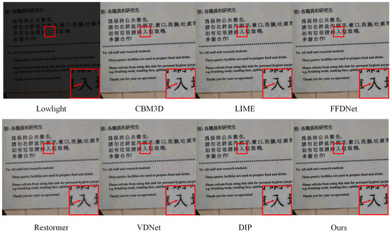
Figure 10.
Visual comparison of the denoised images generated from different methods on the low-light image.
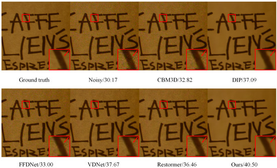
Figure 11.
Visual comparison of the denoised images for the camera RAW image. The quantitative PSNR results are listed behind the noisy and denoised images.
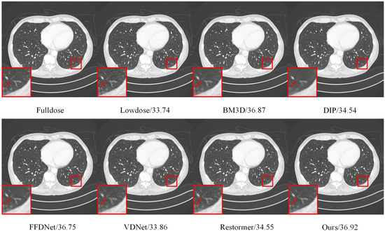
Figure 12.
Visual comparison of the denoised images for the low-dose X-ray image. The quantitative PSNR results are listed behind the noisy and denoised images.
5. Conclusions
This paper proposed a two-stage unsupervised DIP-based denoising method. Unlike the DIP method that uses a given noisy image as the learning target, the proposed method developed a two-target DIP learning strategy to generate intermediate denoised images. The cleaner preliminary image used in two-target DIP learning can help reduce the search space, thereby improving the denoising result. Furthermore, to utilize the uncertainty of the DIP learning, an up- and down-sampling strategy was adopted to generate multiple cleaner preliminary images, which were used to produce multiple intermediate denoised images that were complementary to the image details. Finally, this paper proposed an unsupervised fusion network to fuse the intermediate denoised images into one denoised image to further improve the denoising effect. Extensive experiments on public datasets indicate that the proposed method can considerably improve the denoising effect and perform significantly better than state-of-the-art denoising methods, particularly in real-world image denoising. The proposed method used both external and internal priors. The external prior can recover the general contents of the given noisy image, and the internal prior can effectively restore specific details. Therefore, the proposed method can significantly improve the denoised effect and provide a flexible solution for various noisy images of real scenes.
Author Contributions
Conceptualization, S.X.; Funding acquisition, S.X. and Y.T.; Methodology, S.X. and S.J.; Software, X.C. (Xiaojun Chen) and N.X.; Validation, X.C. (Xiaojun Chen) and X.C. (Xiaohui Cheng); Supervision, S.X.; Writing—original draft, Y.T.; Writing—review and editing, Y.T. and S.X. All authors have read and agreed to the published version of the manuscript.
Funding
This work was funded by the National Natural Science Foundation of China under Grant No. 62162042 and No. 62162043, and in part by the Jiangxi Postgraduate Innovation Special Fund Project under Grant YC2022-s033.
Institutional Review Board Statement
Not applicable.
Informed Consent Statement
Not applicable.
Data Availability Statement
Data sharing not applicable to this article as no datasets were generated during the current study.
Conflicts of Interest
The authors declare that they have no conflict of interest. The manuscript was written with contributions from all authors. All authors have approved the final version of the manuscript.
References
- Dabov, K.; Foi, A.; Katkovnik, V.; Egiazarian, K. Image denoising by sparse 3-D transform-domain collaborative filtering. IEEE Trans. Image Process. 2007, 16, 2080–2095. [Google Scholar] [CrossRef] [PubMed]
- Buades, A.; Coll, B.; Morel, J.M. A non-local algorithm for image denoising. In Proceedings of the IEEE Conference on Computer Vision and Pattern Recognition, San Diego, CA, USA, 20–25 June 2005; pp. 60–65. [Google Scholar]
- Gu, S.; Zhang, L.; Zuo, W.; Feng, X. Weighted nuclear norm minimization with application to image denoising. In Proceedings of the IEEE Conference on Computer Vision and Pattern Recognition, Columbus, OH, USA, 23–28 June 2014; pp. 2862–2869. [Google Scholar]
- Zhang, K.; Zuo, W.; Chen, Y.; Meng, D.; Zhang, L. Beyond a gaussian denoiser: Residual learning of deep CNN for image denoising. IEEE Trans. Image Process. 2017, 26, 3142–3155. [Google Scholar] [CrossRef] [PubMed]
- Zhang, K.; Zuo, W.; Zhang, L. FFDNet: Toward a fast and flexible solution for CNN-based image denoising. IEEE Trans. Image Process. 2018, 27, 4608–4622. [Google Scholar] [CrossRef]
- Zhong, Y.; Liu, L.; Zhao, D.; Li, H. A generative adversarial network for image denoising. Multimed. Tools Appl. 2020, 79, 16517–16529. [Google Scholar] [CrossRef]
- Guo, S.; Yan, Z.; Zhang, K.; Zuo, W.; Zhang, L. Toward convolutional blind denoising of real photographs. In Proceedings of the IEEE/CVF Conference on Computer Vision and Pattern Recognition (CVPR), Long Beach, CA, USA, 15–20 June 2019; pp. 1712–1722. [Google Scholar]
- Ronneberger, O.; Fischer, P.; Brox, T. U-Net: Convolutional networks for biomedical image segmentation. In Proceedings of the International Conference on Medical Image Computing and Computer-Assisted Intervention (MICCAI), Munich, Germany, 5–9 October 2015; pp. 234–241. [Google Scholar]
- Liu, D.; Wen, B.; Fan, Y.; Loy, C.C.; Huang, T.S. Non-local recurrent network for image restoration. In Proceedings of the 32nd Conference on Neural Information Processing Systems (NeurIPS), Montreal, PQ, Canada, 2–8 December 2018; pp. 1673–1682. [Google Scholar]
- Liu, P.; Zhang, H.; Zhang, K.; Lin, L.; Zuo, W. Multi-level wavelet-CNN for image restoration. In Proceedings of the IEEE/CVF Conference on Computer Vision and Pattern Recognition Workshops (CVPRW), Salt Lake City, UT, USA, 18–22 June 2018; pp. 886–895. [Google Scholar]
- Liang, J.; Cao, J.; Sun, G.; Zhang, K.; Gool, L.V.; Timofte, R. SwinIR: Image restoration using swin transformer. arXiv 2021, arXiv:2108.10257. [Google Scholar]
- Zamir, S.W.; Arora, A.; Khan, S.; Hayat, M.; Khan, F.S.; Yang, M.H. Restormer: Efficient transformer for high-resolution image restoration. arXiv 2021, arXiv:2111.09881. [Google Scholar]
- Jagatap, G.; Hegde, C. High dynamic range imaging using deep image priors. In Proceedings of the IEEE International Conference on Acoustics, Speech and Signal Processing (ICASSP), Barcelona, Spain, 4–8 May 2020; pp. 9289–9293. [Google Scholar]
- Sun, H.; Peng, L.; Zhang, H.; He, Y.; Cao, S.; Lu, L. Dynamic PET image denoising using deep image prior combined with regularization by denoising. IEEE Access 2021, 9, 52378–52392. [Google Scholar] [CrossRef]
- Lehtinen, J.; Munkberg, J.; Hasselgren, J.; Laine, S.; Karras, T.; Aittala, M.; Aila, T. Noise2noise: Learning image restoration without clean data. arXiv 2018, arXiv:1803.04189. [Google Scholar]
- Krull, A.; Buchholz, T.O.; Jug, F. Noise2void-learning denoising from single noisy images. In Proceedings of the IEEE Conference on Computer Vision and Pattern Recognition, Long Beach, CA, USA, 15–20 June 2019; pp. 2129–2137. [Google Scholar]
- Batson, J.; Royer, L. Noise2self: Blind denoising by self-supervision. In Proceedings of the International Conference on Machine Learning (ICML), Long Beach, CA, USA, 10–15 June 2019; pp. 524–533. [Google Scholar]
- Moran, N.; Schmidt, D.; Zhong, Y.; Coady, P. Noisier2noise: Learning to denoise from unpaired noisy data. In Proceedings of the IEEE/CVF Conference on Computer Vision and Pattern Recognition (CVPR), Seattle, WA, USA, 13–19 June 2020; pp. 12061–12069. [Google Scholar]
- Xu, J.; Huang, Y.; Cheng, M.M.; Liu, L.; Zhu, F.; Xu, Z.; Shao, L. Noisy-as-clean: Learning self-supervised from corrupted image. IEEE Trans. Image Process. 2020, 29, 9316–9329. [Google Scholar] [CrossRef] [PubMed]
- Pang, T.; Zheng, H.; Quan, Y.; Ji, H. Recorrupted-to-recorrupted: Unsupervised deep learning for image denoising. In Proceedings of the IEEE Conference on Computer Vision and Pattern Recognition, Nashville, TN, USA, 20–25 June 2021; pp. 2043–2052. [Google Scholar]
- Quan, Y.; Chen, M.; Pang, T.; Ji, H. Self2self with dropout: Learning self-supervised denoising from single image. In Proceedings of the 2020 IEEE/CVF Conference on Computer Vision and Pattern Recognition (CVPR), Seattle, WA, USA, 13–19 June 2020; pp. 1887–1895. [Google Scholar]
- Huang, T.; Li, S.; Jia, X.; Lu, H.; Liu, J. Neighbor2neighbor: Self-supervised denoising from single noisy images. In Proceedings of the IEEE Conference on Computer Vision and Recognition, Nashville, TN, USA, 20–25 June 2021; pp. 14781–14790. [Google Scholar]
- Ulyanov, D.; Vedaldi, A.; Lempitsky, V. Deep image prior. In Proceedings of the IEEE Conference on Computer Vision and Pattern Recognition, Salt Lake City, UT, USA, 18–23 June 2018; pp. 9446–9454. [Google Scholar]
- Haris, M.; Shakhnarovich, G.; Ukita, N. Deep back-projection networks for single image super-resolution. IEEE Trans. Pattern Anal. Mach. Intell. 2021, 43, 4323–4337. [Google Scholar] [CrossRef] [PubMed]
- Mou, C.; Zhang, J.; Wu, Z.Y. Dynamic attentive graph learning for image restoration. arXiv 2021, arXiv:2109.06620. [Google Scholar]
- Ren, C.; He, X.; Wang, C.; Zhao, Z. Adaptive consistency prior based deep network for image denoising. In Proceedings of the 2021 IEEE/CVF Conference on Computer Vision and Pattern Recognition (CVPR), Nashville, TN, USA, 20–25 June 2021; pp. 8592–8602. [Google Scholar]
- Zhang, K.; Li, Y.; Zuo, W.; Zhang, L.; Gool, L.V.; Timofte, R. Plug-and-play image restoration with deep denoiser prior. arXiv 2020, arXiv:2008.13751. [Google Scholar] [CrossRef]
- Zhang, K.; Zuo, W.; Gu, S.; Zhang, L. Learning deep CNN denoiser prior for image restoration. In Proceedings of the IEEE Conference on Computer Vision and Pattern Recognition, Honolulu, HI, USA, 21–26 July 2017; pp. 3929–3938. [Google Scholar]
- Bevilacqua, M.; Roumy, A.; Guillemot, C.; Alberi-Morel, M. Low-complexity single-image super-resolution based on nonnegative neighbor embedding. In Proceedings of the British Machine Vision Conference (BMVC), Guildford, UK, 3–7 September 2012; pp. 135.1–135.10. [Google Scholar]
- Martin, D.; Fowlkes, C.; Tal, D.; Malik, J. A database of human segmented natural images and its application to evaluating segmentation algorithms and measuring ecological statistics. Proceddings of the IEEE International Conference on Computer Vision, Vancouver, BC, Canada, 7–14 July 2001; pp. 416–423. [Google Scholar]
- Xu, S.; Chen, X.; Luo, J.; Cheng, X.; Xiao, N. An unsupervised fusion network for boosting denoising performance. J. Vis. Commun. Image Represent. 2022, 88, 103626. [Google Scholar] [CrossRef]
- Yu, L.; Luo, J.; Xu, S.; Chen, X.; Xiao, N. An unsupervised weight map generative network for pixel-level combination of image denoisers. Appl. Sci. 2022, 12, 6227. [Google Scholar] [CrossRef]
- Yue, Z.; Yong, H.; Zhao, Q.; Meng, D.; Zhang, L. Variational denoising network: Toward blind noise modeling and removal. In Proceedings of the 33rd Conference on Neural Information Processing Systems (NeurIPS), Vancouver, BC, Canada, 8–14 December 2019. [Google Scholar]
- Guo, X.; Yu, L.; Ling, H. LIME: Low-light image enhancement via illumination map estimation. IEEE Trans. Image Process. 2017, 26, 982–993. [Google Scholar] [CrossRef] [PubMed]
- Cai, J.; Gu, S.; Zhang, L. Learning a deep single image contrast enhancer from multi-exposure images. IEEE Trans. Image Process. 2018, 27, 2049–2062. [Google Scholar] [CrossRef] [PubMed]
- Nam, S.; Hwang, Y.; Matsushita, Y.; Kim, S.J. A holistic approach to cross-channel image noise modeling and its application to image denoising. In Proceedings of the IEEE Conference on Computer Vision and Pattern Recognition (CVPR), Las Vegas, NV, USA, 27–30 June 2016; pp. 1683–1691. [Google Scholar]
- Yang, Q.; Yan, P.; Zhang, Y.; Yu, H.; Shi, Y.; Mou, X.; Kalra, M.K.; Zhang, Y.; Sun, L.; Wang, G. Low-dose CT image denoising using a generative adversarial network with wasserstein distance and perceptual loss. IEEE Trans. Med. Imaging 2018, 37, 1348–1357. [Google Scholar] [CrossRef] [PubMed]


Publisher’s Note: MDPI stays neutral with regard to jurisdictional claims in published maps and institutional affiliations. |
© 2022 by the authors. Licensee MDPI, Basel, Switzerland. This article is an open access article distributed under the terms and conditions of the Creative Commons Attribution (CC BY) license (https://creativecommons.org/licenses/by/4.0/).