Article

Hybrid Genetic Algorithm−Based BP Neural Network Models Optimize Estimation Performance of Reference Crop Evapotranspiration in China

1
State Key Laboratory of Aridland Crop Science, Gansu Agricultural University, Lanzhou 730070, China
2
Institute of Farmland Irrigation, Chinese Academy of Agricultural Sciences, Key Laboratory of Crop Water Use and Regulation, Ministry of Agriculture and Rural Affairs, Xinxiang 453002, China
3
College of Software, Henan Normal University, Xinxiang 453007, China
*
Author to whom correspondence should be addressed.
Appl. Sci. 2022, 12(20), 10689; https://doi.org/10.3390/app122010689
Submission received: 15 September 2022 / Revised: 11 October 2022 / Accepted: 19 October 2022 / Published: 21 October 2022
(This article belongs to the Special Issue Advanced Plant Biotechnology in Sustainable Agriculture)

Abstract

:
Precise estimation of reference evapotranspiration (ET0) is of significant importance in hydrologic processes. In this study, a genetic algorithm (GA) optimized back propagation (BP) neural network model was developed to estimate ET0 using different combinations of meteorological data across various climatic zones and seasons in China. Fourteen climatic locations were selected to represent five major climates. Meteorological datasets in 2018–2020, including maximum, minimum and mean air temperature (Tmax, Tmin, Tmean, °C) and diurnal temperature range (∆T, °C), solar radiation (Ra, MJ m−2 d−1), sunshine duration (S, h), relative humidity (RH, %) and wind speed (U2, m s−1), were first subjected to correlation analysis to determine which variables were suitable as input parameters. Datasets in 2018 and 2019 were utilized for training the models, while datasets in 2020 were for testing. Coefficients of determination (r2) of 0.50 and 0.70 were adopted as threshold values for selection of correlated variables to run the models. Results showed that U2 had the least r2 with ET0, followed by ∆T. Tmax had the greatest r2 with ET0, followed by Tmean, Ra and Tmin. GA significantly improved the performance of BP models across different climatic zones, with the accuracy of GABP models significantly higher than that of BP models. GABP0.5 model (input variables based on r2 > 0.50) had the best ET0 estimation performance for different seasons and significantly reduced estimation errors, especially for autumn and winter seasons whose errors were larger with other BP and GABP models. GABP0.5 model using radiation/temperature data is highly recommended as a promising tool for modelling and predicting ET0 in various climatic locations.

1. Introduction

Reference crop evapotranspiration (ET0) is a predominant factor in hydrologic processes and a prerequisite for calculation of crop water requirements [1,2]. In recent years, model estimation of ET0 has been a major way to obtain ET0 due to its low cost and acceptable accuracy [3]. With solar radiation and aerodynamic factors considered, FAO Penman–Monteith (PM) model has been a reference method for computing ET0 [4]. However, access to full meteorological datasets (i.e., air temperature, solar radiation, sunshine hours, wind speed and vapor pressure etc.) is not always easy in numerous developing nations, making the practice of PM model limited in many countries [5]. Radiation and temperature data are the commonest meteorological data obtained by weather stations. Many studies also reported that radiation and temperature were the factors most correlated to ET0 [6,7]. How to efficiently obtain higher precision ET0 estimation models using less data has been an urgent problem to be solved.
ET0 estimation models are divided into two main categories: empirical models and machine learning models. Empirical models are site–specific, needing modifications for different locations [8]. In this context, it is difficult to select a broadly adopted empirical model suitable everywhere [9]. Recently, machine learning models have been successfully implemented to predict the ET0 [10]. Artificial neural network (ANN) uses the interconnected information processing units to turn meteorological inputs into ET0 outputs and has been regarded as one of the best approaches to predict ET0 [11]. For example, neural network models have been proposed to compute ET0 in the Beas–Sutlej basin, India [12] and in the Peloponnese Peninsula, Greece [13], based on different combinations of input data and they concluded that neural network models showed good performance in ET0 prediction. In the tropical climate of Brazil, neural networks performed better in ET0 prediction with limited meteorological data than support vector machine (SVM) models [14]. In Victoria, Australia, only temperature and wind speed data were adopted to predict ET0 using artificial and wavelet neural networks and it was reported that both models predicted ET0 with good accuracy [15].
The back propagation network (BP) model is one of the most popularly adopted neural network models due to its simple structure and easy implementation. Several studies have been adopting BP neural networks to predict ET0 [16,17]. In Florida, USA, regional ET0 was predicted using BP models in a continental climate and it had good consistency with the measured ET0 [18]. In India, the accuracy of BP models was verified in a subtropical monsoon climate and was proved effective in ET0 prediction [19]. However, the BP neural network has some drawbacks, which makes it easy to fall into local optimal solution [20]. Some scholars found that local extremum was easily produced by the BP neural network, yielding low applicability among various climatic locations [21,22]. Several studies have reported that climatic types exerted significant effect on the performance of BP models. For example, the accuracy of BP models for ET0 estimation was lower in the monsoon plateau than in subtropical climate due to its difference in sensitivity to radiation and temperature [23]. Furthermore, BP models were shown to have greater biases in ET0 estimation in cold seasons than in warm seasons [24,25]. The uncertainty in ET0 estimation across different climatic zones was probably due to the fact that in tropical regions wind speed was really slow, especially in rainy months, while it was very high in mountain plateau areas [15]. In addition, in tropical regions relative humidity was very high, whereas in arid and semi–arid areas relative humidity was extremely low [4]. All this affects accuracy of ET0 estimation. In data scarce areas, Chen et al. (2015) established ET0 estimation BP models with only temperature input in Hexi Corridor, Northwest China and found that their root mean square error (RMSE) was increased by 23%, compared with Hargreaves equation [26]. Zhang et al. (2015) found that the BP neural network method only with temperature data increased RMSE and mean absolute error (MAE) in the North China Plain (NCP) compared with support vector regression (SVR) models [27].
Recently, various optimized algorithms were developed to improve the performance of neural networks. Genetic algorithm (GA) is an optimized algorithm simulating the nature of biological genetics in a population to search for the best individuals as optimal weights and thresholds for neural networks [28]. GA has been shown to have the capacity to optimize learning machine model using limited data. In Gyeong Sangbuk, South Korea, GA optimized neural networks models were evaluated in predicting the daily ET0 and it was found that GA optimization methods were able to estimate daily ET0 from limited weather data [29]. In Southwest China, Liu et al. (2022) evaluated the performance of extreme learning machine (ELM), a new learning feedforward neural network, GA optimized ELM and empirical models for estimating daily ET0 and found that GA–ELM was the most efficient method for predicting daily ET0 using Tmax, Tmin and Ra data [30]. The accuracy of GA optimized BP model in ET0 prediction also proved higher than that of empirical models under the same parameter input combinations in Yangtze–Huaihe River Basin, China [31]. It is obvious that GA optimization models have been a hot spot in the application of machine learning.
China covers a variety of climate zones and has obvious alternation of seasons. Previous studies of ET0 estimation mainly concentrated on a specific time scale in particular regions of China. This paper used GA optimized BP neural network models to estimate ET0 from 14 locations across China over five climatic zones. Coefficients of determination between meteorological variables and ET0 were calculated. Data input combinations were determined based on r2 > 0.50 and r2 > 0.70, respectively. This study attempted to comprehensively compare BP and GABP models for modeling ET0 using different input combinations across various climatic zones and seasons in China. We hypothesized that GABP models significantly improved model performances across various climatic zones and seasons. This study aims to provide an optimized model for local farmers and policy–makers to accurately estimate and predict potential evapotranspiration and crop water consumption.

2. Materials and Methods
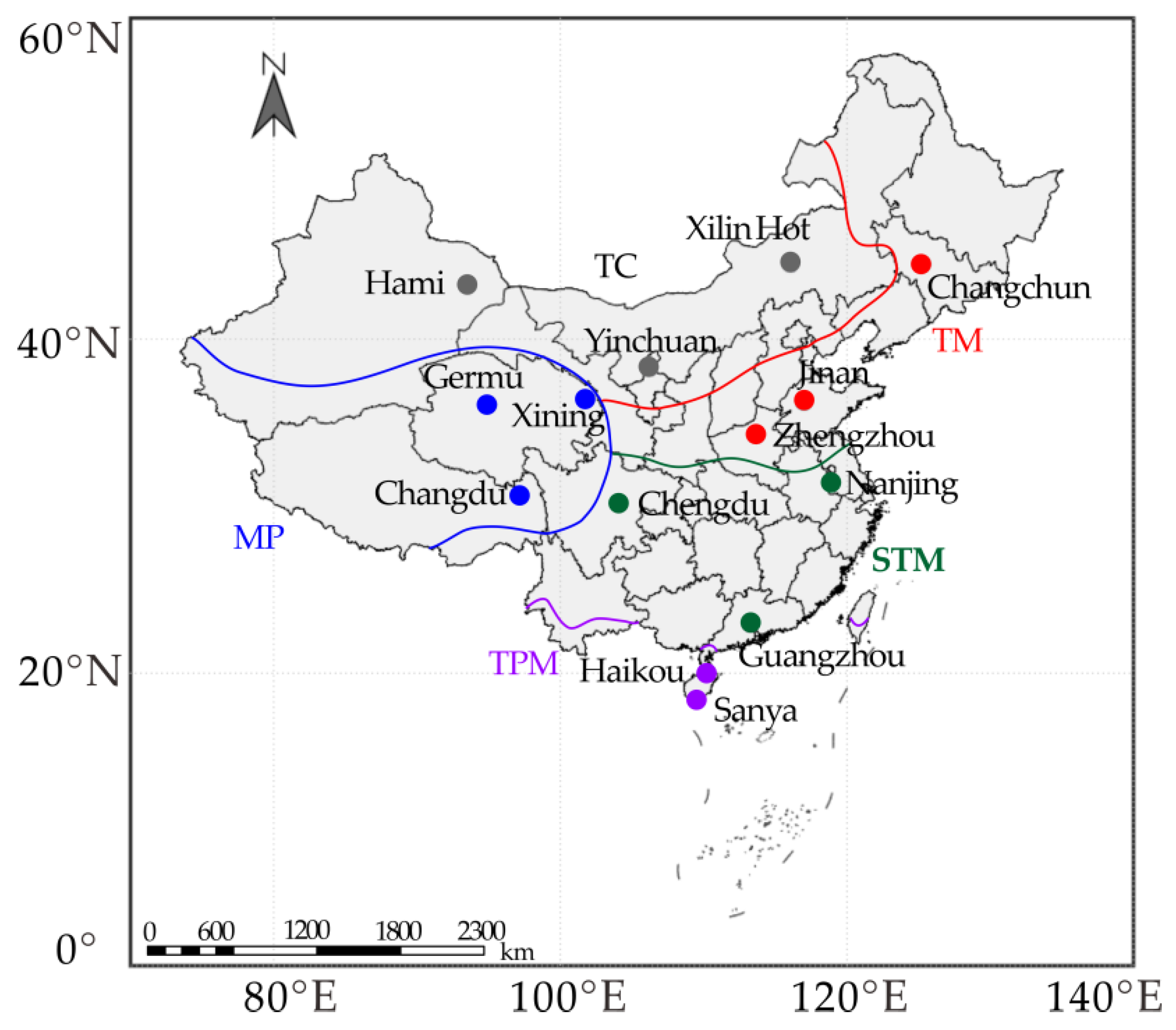
2.1. Study Area

China has an area of 9.6 million square kilometers in eastern Eurasia. According to the characteristics of precipitation, air temperature and solar radiation which markedly vary across China, five climatic zones are divided as follows: (I) temperate continental zone (TC), (II) temperate monsoon zone (TM), (III) mountain plateau zone (MP), (IV) subtropical monsoon zone (STM), (V) tropical monsoon zone (TM) [32]. The selection of climatic sites was based on a previous study by Fan et al. (2018) published in Agricultural and Forest Meteorology [23]. Taking the sites’ distribution in each climatic zone and the distance among locations in account, 14 national meteorological stations established by the China Meteorological Administration (CMA) were selected (Figure 1). The meteorological stations were distributed between latitudes 18°14′–43°56′ N and longitudes 93°31′–125°13′ E, with above sea levels ranging from 7.1 m to 3315 m (Table 1).

2.2. Data Collection and Analysis

In this study, data of daily maximum, minimum, mean temperature (Tmax, Tmin, Tmean, °C), diurnal temperature range (∆T, °C), total solar radiation (Ra, MJ m−2 d−1), actual sunshine duration (S, h), wind speed at 2 m height (U2, m s−1) and relative humidity (RH, %), during the period of 2018–2020 were collected. After the data quality check by the CMA, the datasets were proved to have good continuity and accuracy.

2.3. Models for Estimating Reference Crop Evapotranspiration

2.3.1. FAO Penman–Monteith Model

As a widely accepted model for estimating ET0, the FAO Penman–Monteith equation was employed in this study. It is also considered a standard method to compare the accuracy of other models. The P–M model is described as follows:
E T 0 = 0.408 Δ ( R n G ) + γ 900 T + 273 U 2 ( e s e a ) Δ + γ ( 1 + 0.34 U 2 )
where Δ is the slope of vapor pressure curve (kPa °C−1), Rn is surface net solar radiation (MJ m−2 d−1), G is soil heat flux density (MJ m−2 d−1) and γ is the psychrometric constant (kPa °C−1). T is mean air temperature (°C), a mean value of Tmax and Tmin, U2 is wind speed at 2 m height (m s−1), es is saturation vapor pressure (kPa) and ea is actual vapor pressure (kPa).

2.3.2. BP Neural Network Model

A neural network model with multi–layers is able to approximate any nonlinear continuous function [33]. BP neural network is a nonlinear adaptive learning system, containing lots of parallel interconnected neurons. The advantage of BP neural network is its feed–forward and feed–back structure. A feed–forward network contains an input layer, an output layer and several hidden layers, constructing multiple layers of perceptron network [26]. The BP output results can affect the inputs using the back propagation (BP) principle and, in turn, adjust the weights of the feedback neural network. In this study, we constructed an ‘n–7–1’ structure of a BP neural network. The letter ‘n’ was the number of input variables in different input combinations. Owing to the nature of back propagation, the BP model can feedback the input layers either in a positive or a negative direction, which increases or decrease the weights of networks [29].

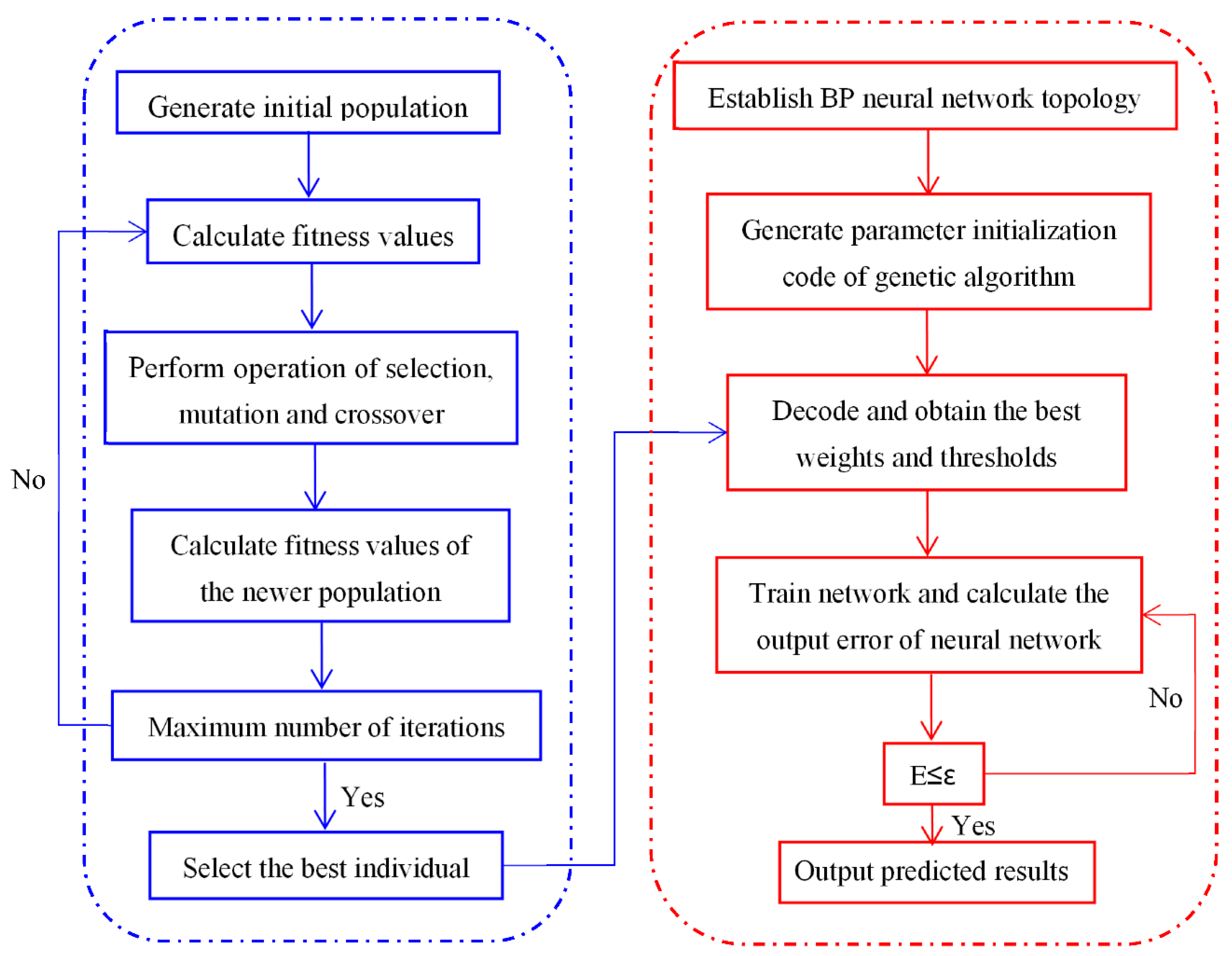
2.3.3. Genetic Algorithm Optimized BP Neural Network Model

Genetic algorithm (GA) makes use of the principle of population evolution and biological genetics in a natural environment [34]. First, GA generates initial population randomly and then performs a series of operations of selection, mutation and crossover to obtain the best fitness values for the populations (Figure 2). The accuracy of training convergence can be significantly improved using GA due to its merits in global searching, parallelism and generalization ability [35]. With fast learning and accurate convergence traits, the GABP neural network model can effectively obtain the optimal weights and thresholds of the network, finding out the global optimal solution with less computational costs [36]. The BP and GABP models were run in Matlab 2018b (MathWorks Inc., Natick, MA, USA).

2.4. Input Variables Selection

According to previous studies, eight variables, including maximum, minimum and mean air temperature (Tmax, Tmin, Tmean, °C), diurnal temperature range (∆T, °C), total solar radiation (Ra, MJ m−2 d−1), actual sunshine duration (S, h), relative humidity (RH, %) and wind speed at 2 m height (U2, m s−1), were initially selected [32,35]. Datasets were chosen from 2018–2020, in which 2018 and 2019 datasets were utilized for training models and datasets fir the year of 2020 were for testing. All the results reported referred to the testing phase. Published literature has shown that the effect of meteorological parameters on the performance of ET0 estimation models varied markedly across different climatic zones [7]. Therefore, correlation analysis was conducted before the variables were applied to neural network models. With the extent of determination coefficients (r2) ranging from 0.10 to 0.93, threshold values were determined using the median (r2 = 0.50) and third quartile (r2 = 0.70) values from a box chart after statistical distribution for training and testing models (Table 2).

2.5. Model Accuracy Evaluation

The accuracy of BP and GABP neural network models were evaluated using four statistical indices, namely the root mean square error (RMSE), correlation coefficient (R), mean absolute error (MAE) and mean bias error (MBE) [37]. Smaller MAE and RMSE suggest lower error between the predicted and measured values. R is used to indicate the correlation between the predictions and observations and is proposed to be sufficiently higher to indicate a better prediction performance [38]. The MBE values higher than 0 indicate over prediction, whereas MBE values lower than 0 mean under prediction. The mathematical equations of the four statistical indices are written as:
R M S E = i = 1 n ( O i P i ) 2 n
R = i = 1 n ( P i P ¯ ) ( O i O ¯ ) i = 1 n ( P i P ¯ ) 2 i = 1 n ( O i O ¯ ) 2
M A E = 1 n i = 1 n | O i P i |
M B E = 1 n i = 1 n ( O i P i )
where n is the number of measured values in testing phase. Pi is predicted values on day i and Oi is observed values on day i. P ¯ represents the mean values of Pi and  O ¯ the mean values of Oi in testing phase.

3. Results

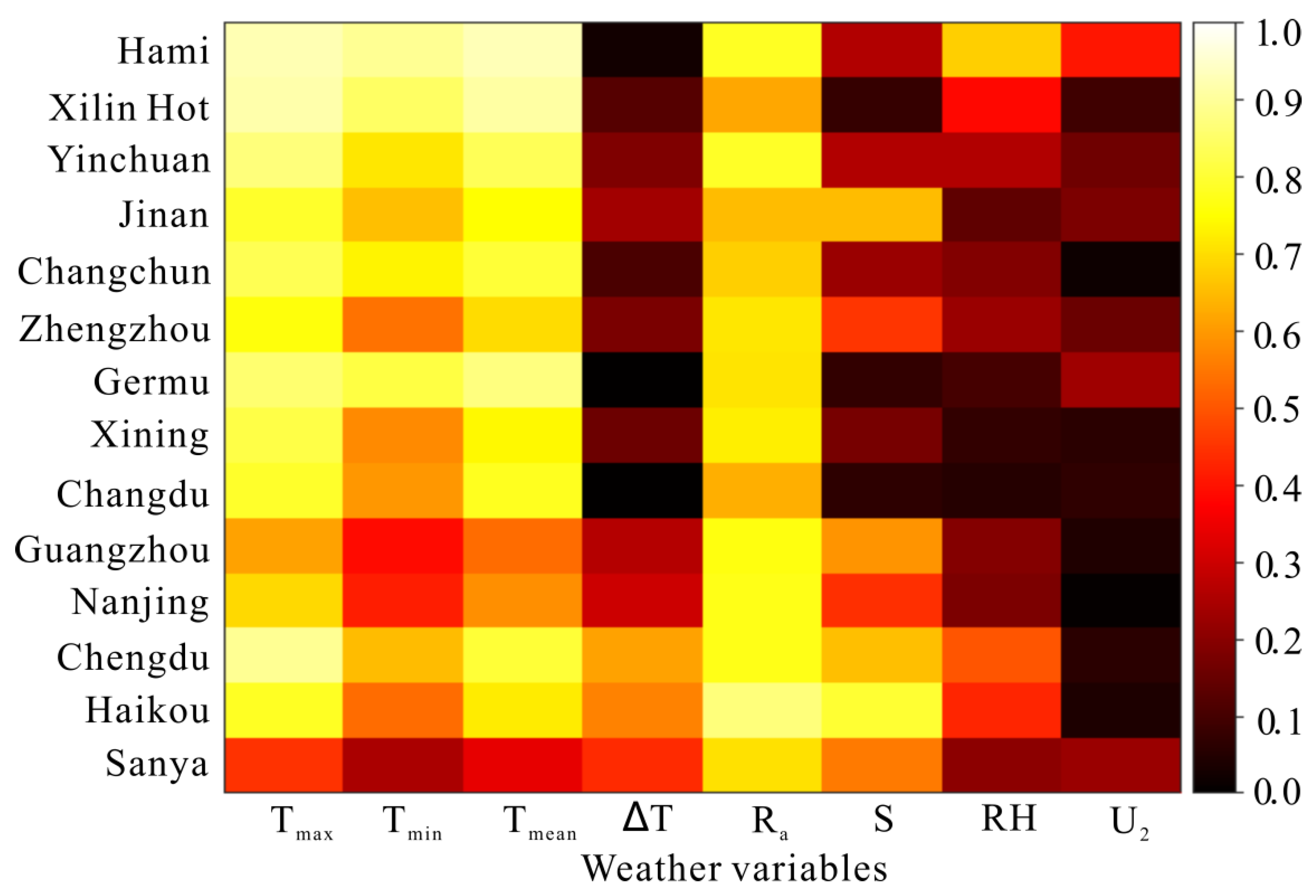
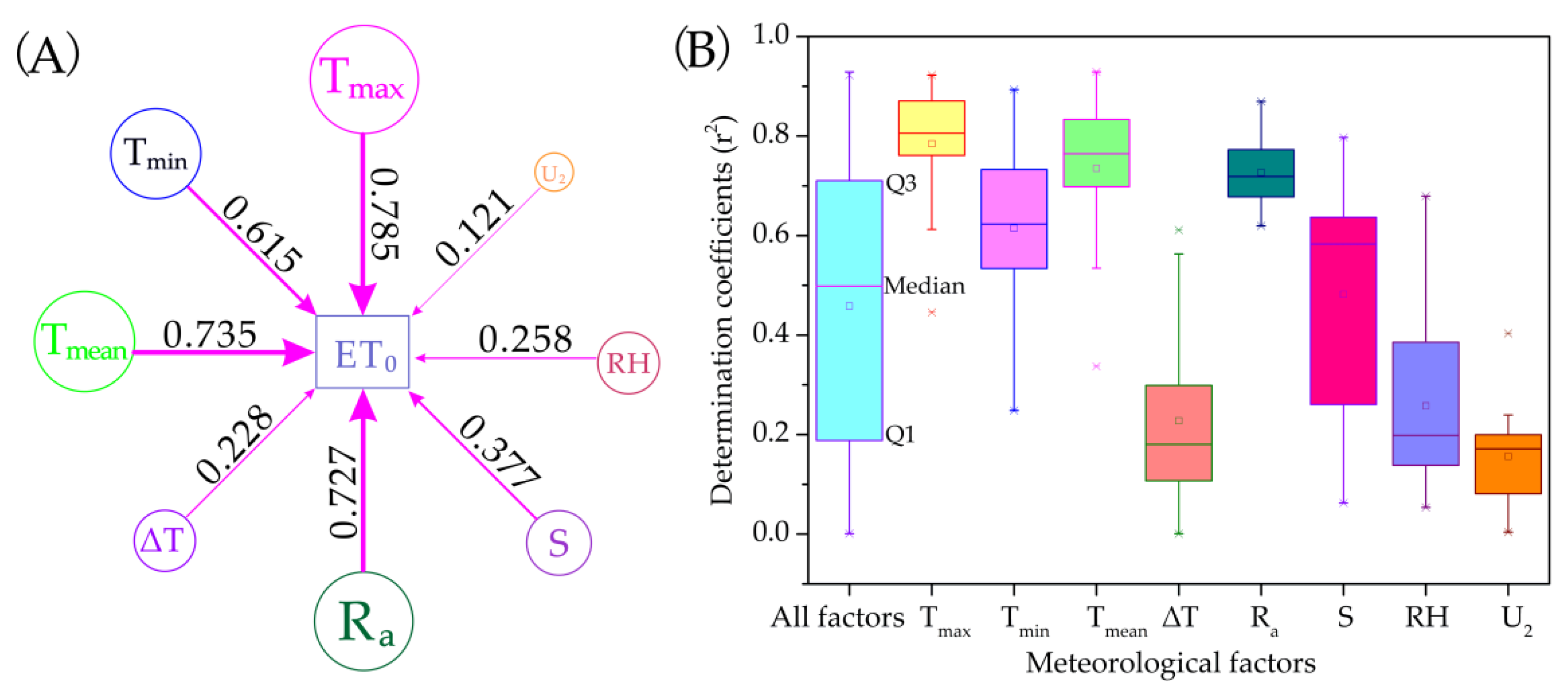
3.1. Correlation Analysis between ET0 and Meteorological Factors

Correlation analysis between FAO PM based ET0 estimates and each input meteorological variable was performed to help identify dominant variables contributing to ET0 variations (Figure 3). Results showed that Tmax had the greatest coefficient of determination (r2), averaging 0.785, followed by Tmean (r2 = 0.735), Ra (r2 = 0.727) and Tmin (r2 = 0.615). In contrast, U2 had the least r2 of 0.125, followed by ∆T (r2 = 0.228), RH (r2 = 0.258) and S (r2 = 0.377). Dataset of U2 were excluded as an input variable due to low r2 values (0.04–0.40). ∆T only correlated with ET0 for tropical and subtropical humid climate, with its r2 ranging from 0.501 (Sanya) to 0.611 (Chengdu). S showed significant correlation with ET0 for tropical, subtropical and temperate monsoon climate, with r2 ranging from 0.551 (Sanya) to 0.797 (Haikou).

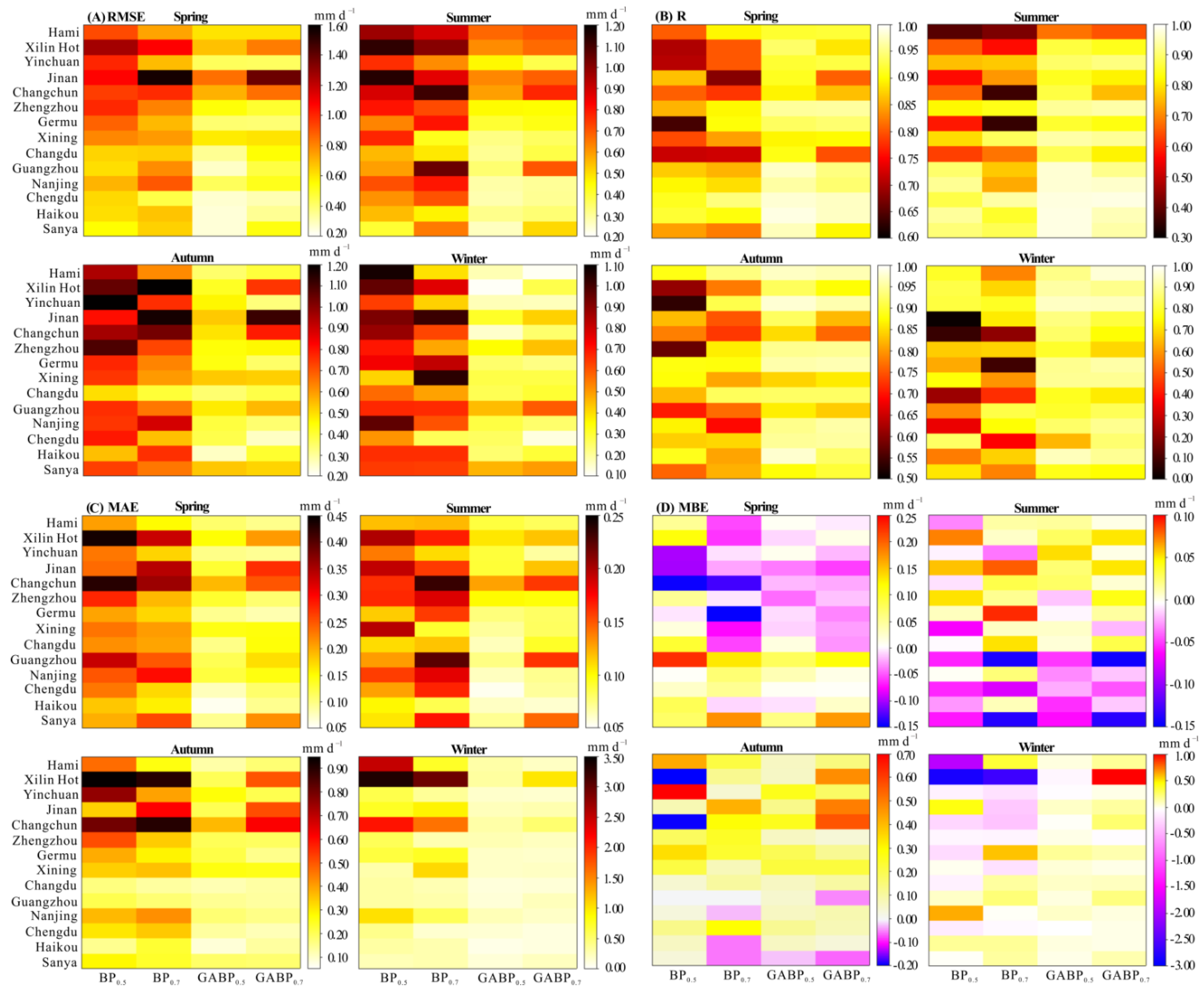
3.2. Comparison of Statistical Indices of BP and GABP Models

The statistical indices in testing phase for BP and GABP neural network models were presented in Figure 4. As indicated by RMSE, R, MAE and MBE, the accuracy for GABP estimation models was higher than that of BP models (Table S1). Mean values of RMSE, R, MAE and MBE were 0.755 mm d−1, 0.724, 0.404 mm d−1 and −0.023 mm d−1, respectively, for BP models and were 0.434 mm d−1, 0.894, 0.169 mm d−1 and 0.053 mm d−1, respectively, for GABP models. Generally, the performance of BP0.5 and BP0.7 models was best in tropical and subtropical monsoon zones, followed by the mountain plateau zone, and worst in temperate monsoon and temperate continental climates, respectively. However, GA significantly improved the performance of BP models for different climatic zones. For example, mean values of RMSE and MAE for GABP models were 0.434 and 0.169 mm d−1, or a decrease of 42% and 58%, respectively, compared to BP models. Mean R values of GABP models were 0.894, or an increase of 23%, compared to BP models. As for MBE values, GABP models significantly decreased the values for tropical, subtropical monsoon and temperate continental zones, but significantly increased MBE values for temperate monsoon zone. It was a surprise that GA showed a contradictory effect on MBE among climatic types. Low mean MBE may be a result of an average of both positive and negative values, which may not indicate an approximation of true values. In this study, mean MBE value was low for BP0.7 model but it was true that large difference existed in both negative and positive MBE values during different seasons for the BP0.7 model. On the contrary, more neutral values of MBE for the GABP0.5 model indicated a better estimation accuracy than did the BP0.5, BP0.7 and GABP0.7 models. In this study, seasonal factor was considered in the comparison of statistical indices. Mean value of R was lowest (0.690) for winter season, whereas it was 0.812 to 0.877 for the other three seasons. Mean values of MAE were highest for winter (0.529 mm d−1), intermediate for autumn (0.309 mm d−1) and least for spring and summer seasons. RMSE values followed a similar order to MAE. However, GA significantly reduced RMSE and MAE across different seasons. For example, averaged RMSE and MAE values of GABP models for winter season were 0.292 mm d−1 and 0.236 mm d−1, or a decrease of 57% and 71%, compared to BP models, whereas the R value of GABP models was 0.841, or an increase of 56%, compared to BP models.

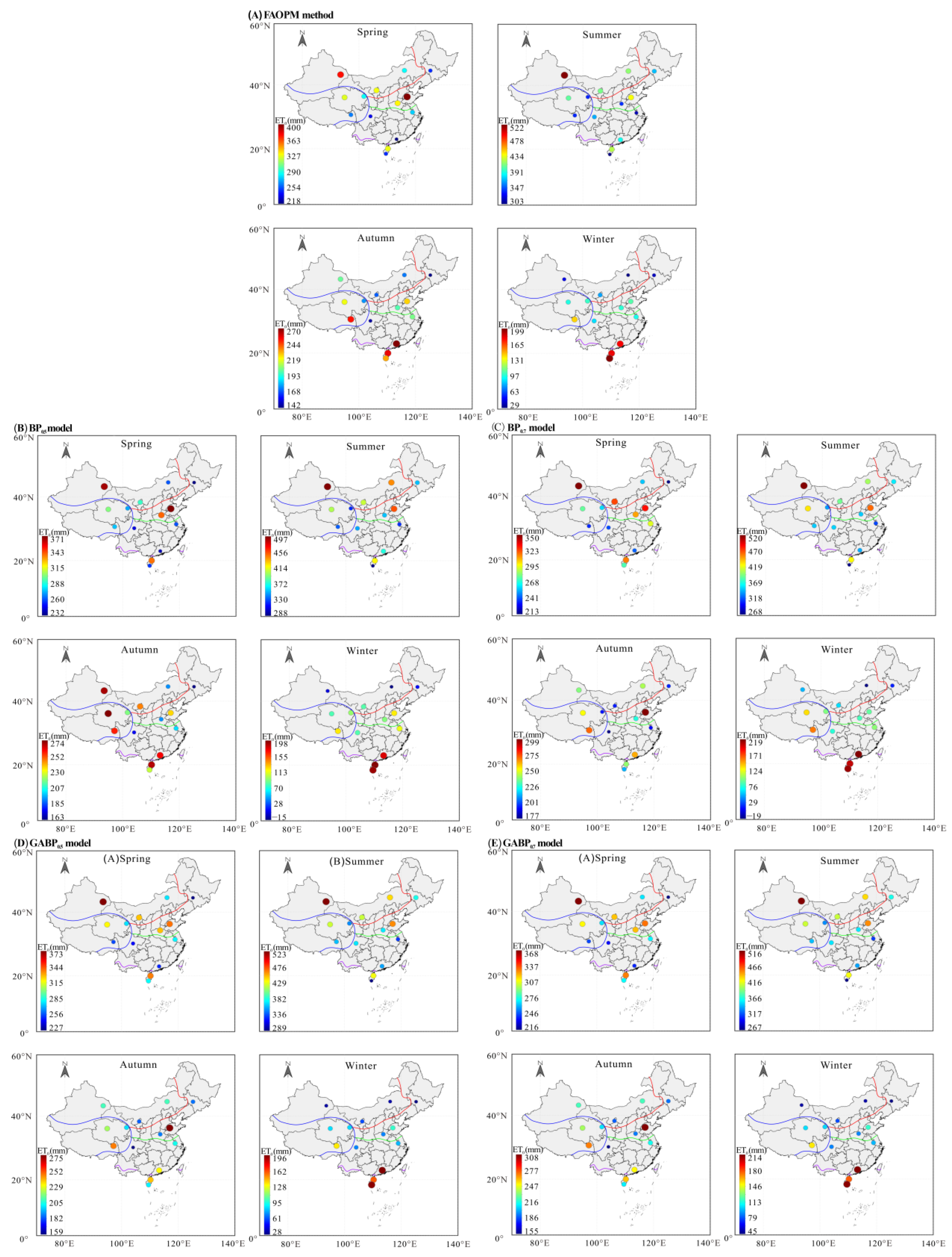
3.3. Comparison of Seasonal ET0 Estimates from FAO PM Equation, BP and GABP Models

During model training and testing phase, ET0 was estimated at a daily time step. Figures S1–S4 show the results of the daily ET0 trends of FAO PM equation vs. trends of BP and GABP models during testing phase. These daily estimated ET0 data were accumulated as seasonal ET0 data for comparison. Based on FAO PM equation, annual ET0 was greatest for TPM zone (1088 mm yr−1), intermediate for TC zone (1014 mm yr−1) and MP zone (1012 mm yr−1) and least for TM zone (984 mm yr−1) and STM zone (930 mm yr−1) (Table 3). Model performance in seasonal ET0 estimates varied markedly across various seasons (Figure 5). BP and GABP models underestimated seasonal ET0 in spring by −2.27% to −5.07%, overestimated ET0 in autumn by 6.05% to 10.1% and well estimated ET0 in summer (−1.50% to −0.66%). In winter season, BP0.5 model underestimated ET0 by −6.38% while GABP0.7 models overestimated ET0 by 6.69%. In contrast, GABP0.5 model well estimated seasonal ET0 in spring, summer and winter seasons (−0.55% to −1.27%). The greatest ET0 overestimation (by 10.1%) was observed in autumn for BP models, while GABP0.5 model appreciably decreased the overestimation to 6.05% in autumn. BP0.5 and BP0.7 models overestimated seasonal ET0 in autumn by 14.2% to 33.5% in TC zone, which was unacceptable. Through comparison, GABP0.5 model had the best model performance in seasonal ET0 estimation, especially for autumn and winter seasons, with large discrepancy for other models.

3.4. Result Analysis

In general, correlation analysis was the first step for ET0 estimation, because it determined which variables were qualified as an input factor. Our results showed that air temperature and solar radiation were the dominant factors contributing to ET0. Other factors such as ∆T, RH and S were only correlated with ET0 in specific climates or cities. The second step was to calculate threshold values of r2 for the selection of input variables. With no methodology to refer to, we subjected all r2 of meteorological factors to statistical distribution using a box chart (Figure 6) and then used median (r2 = 0.50) and third quartile values (r2 = 0.70) as thresholds. Correlated factors satisfying the thresholds were applied to BP and GABP models. Our study may provide a reference for the selection of input variables. Significant climatic and seasonal effects was observed on ET0 estimation. BP models performed worse in cold seasons and in arid to semi–arid climates. However, GABP models significantly improved model performance even with fewer input parameters. In general, GABP0.7 model was acceptable in annual ET0 estimation, while GABP0.5 performed best in seasonal ET0 estimation.

4. Discussion

4.1. Contribution of Meteorological Factors to ET0 Variations

Neural network models usually need a variety of meteorological factors to train and test [38]. However, adequate weather parameters are often inaccessible in many developing countries [3]. Determining dominant influencing factors helps improve model working efficiency and popularity. Previous studies showed that variables such as air temperature and solar radiation explained approximately 70% of the contribution to ET0 variations [39,40]. Our study showed that the correlation between ET0 and air temperature and between ET0 and solar radiation was highest, while ∆T, RH and U2 had significantly low r2 (Figure 6A). The result was consistent with the findings of Qiu et al. (2019), who regarded energy–related factors as the most influencing variables for ET0 [35]. In previous studies, several scholars considered diurnal temperature range (∆T, °C) a dominant input variable for calculating ET0 [7,41], which was inconsistent with our study. In this study, ∆T showed less correlation at most sites. The r2 between ∆T and ET0 was 0.50 in Sanya and Haikou, where their ∆T was less than 10 °C in most seasons due to a tropical climate [42]. Smaller ∆T usually indicates closer values to Tmax and Tmin. When ∆T becomes larger, ET0 shows more correlation with Tmax and Tmin but less with ∆T because large data fluctuation is considered undesirable in the correlation analysis [43,44]. In this study, U2 was the least correlated factor. The reason may be that wind speed is not a dominant factor in the atmospheric energy cycle [45,46,47]. Besides, U2 is further impacted by land use and topography, making accurate data difficult to obtain [48]. This is why several simplified ET0 models do not include U2 as an input variable [49,50].

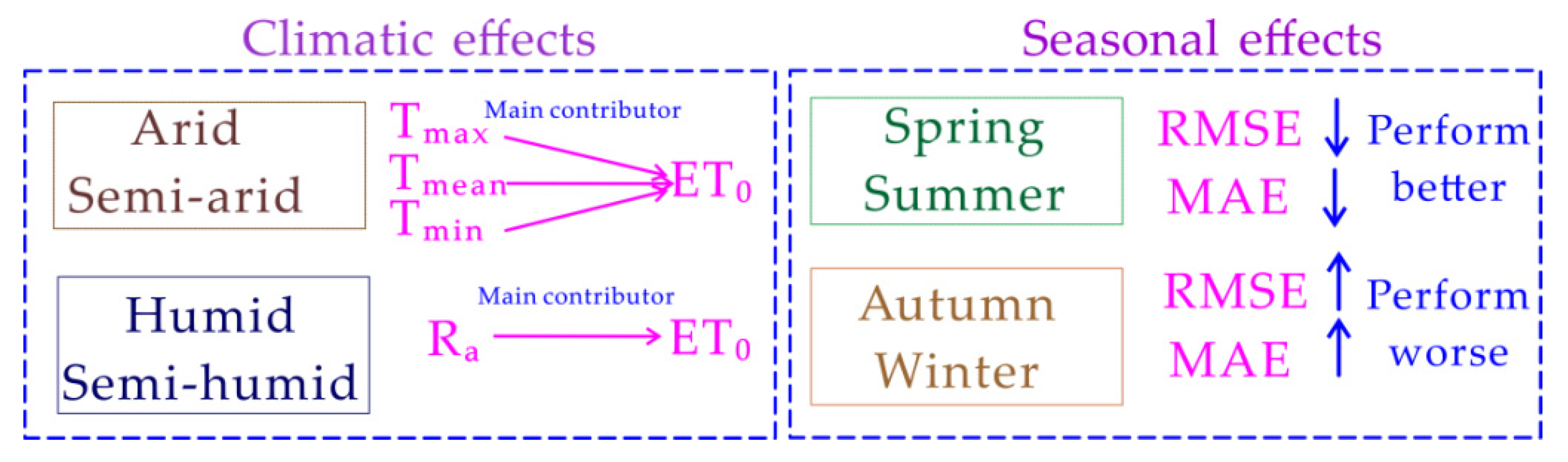
4.2. Seasonal and Climatic Effects on ET0 Estimation

Our study found that ET0 in arid and semi–arid climate was more affected by air temperature, while solar radiation affected ET0 more in humid and semi–humid climate (Figure 7). Several previous literature also found that the sensitivity of meteorological factors to ET0 varied across climatic types [51,52,53,54]. When seasonal ET0 was compared, the accuracy of ET0 estimation decreased in autumn and winter seasons, especially for BP models in TC and PM zones. In Shaanxi Province, Northwest China, six sites were selected to represent semi–humid to arid climates to compare the performance of BP models and similar results were observed to our study. It was found that average relative error (ARE) was greater than 12% in autumn and winter seasons, especially for arid climate in North Shaanxi province [55]. In central China, worse model performance was also found during autumn and winter seasons, while the ARE was smaller (<9%) for a subtropic monsoon climate whose air temperature and relative humidity were relatively higher [56]. The reason why ET0 estimates had greater discrepancy in cold seasons and areas might be attributable to its large ∆T as indicated by the extremely low correlation with ∆T (°C) in temperate continental and mountain plateau zones.

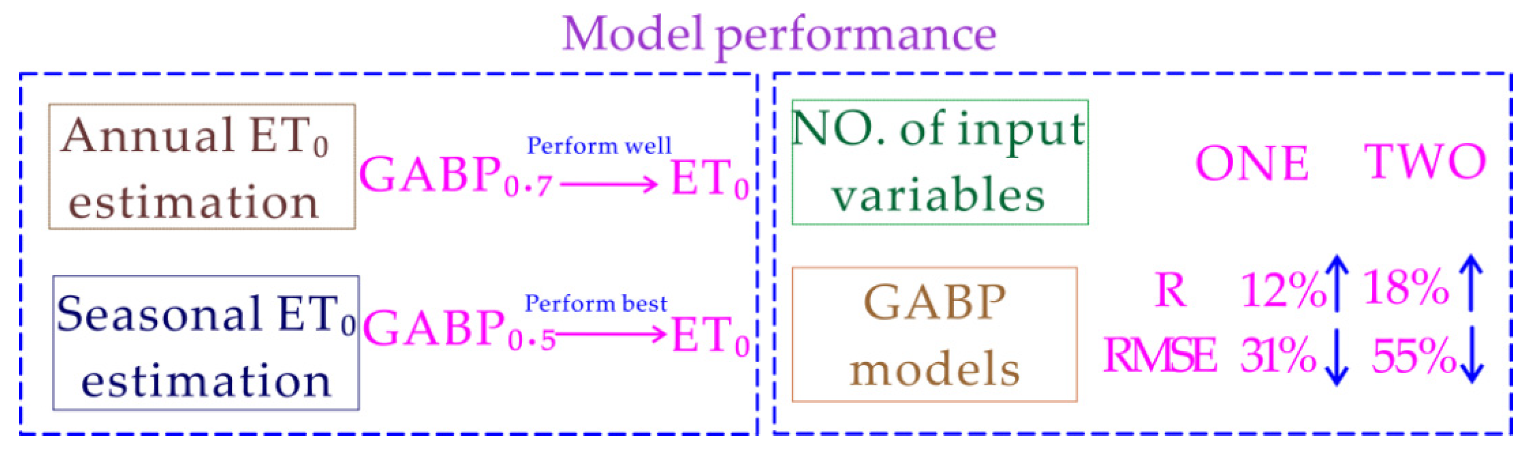
4.3. Genetic Algorithm Improves the Performance of Models

Previous studies reported that performance of neural network models became worse with limited input variables [57,58]. However, genetic algorithm (GA) was able to improve the performance of models with fewer input factors [59,60]. In northern Greece, it was found that ANN models with fewer inputs gave rise to lower accuracy than the GA optimized ANN model [61]. In South Korea, it was reported that GABP models estimated daily ET0 with acceptable accuracy using only temperature data [29]. In Yangtze River Basin, China, the accuracy of GABP models was also proved higher than that of empirical models with fewer parameter inputs [31]. When choosing r2 = 0.70 as a threshold value, the number of input variables for BP0.7 and GABP0.7 models were only one for Guangzhou (Ra) and Sanya (Ra) and two for Nanjing (Tmax and Ra) and Jinan (Tmax and Tmean), respectively. With the same input variables, R of GABP models was increased by 12–18% for the above mentioned cities. Moreover, RMSE of GABP models was decreased by 31–55% for Guangzhou and Sanya cities (Figure 8). Our results clearly indicated that GABP models obtained more accuracy than did the BP models with fewer parameters. Specifically, for annual ET0 estimation, the GABP0.7 model using less input variables performed well with acceptable accuracy, whereas the GABP0.5 model was preferable for seasonal ET0 estimation.

5. Conclusions

In this study, based on the collected datasets from the 14 national meteorological stations in China, BP and GABP models were developed to estimate daily ET0 across different climatic zones and seasons. Correlation analysis between ET0 and meteorological parameters helped determine the most commonly influencing variables applied to neural network models. U2 had the least r2 with ET0, followed by ∆T. Tmax had the greatest r2 with ET0, followed by Tmean, Ra and Tmin. Median and third quartile values of r2 = 0.50 and 0.70 were adopted as threshold values for the selection of input variables. The results showed that the GABP0.5 model using radiation and temperature data had a better performance than the GABP0.7 model in autumn and winter seasons and GABP models were superior to BP models in ET0 estimation. Although GABP0.7 model produced less accuracy than the GABP0.5 model, it outperformed both the BP0.5 and BP0.7 models. When seasonal differences were taken into account, the GABP0.5 model outperformed the GABP0.7 model. Our study clearly addressed the hypothesis that GABP models significantly improved model performance in annual ET0 estimation across various climatic zones and seasons. It was concluded that the GABP0.5 model can be used for irrigation engineers and agricultural practitioners to estimate ET0 for efficient crop water requirement calculation and can be a useful tool to be adopted in smart irrigation in different climatic zones in China.

Supplementary Materials

The following supporting information can be downloaded at: https://www.mdpi.com/article/10.3390/app122010689/s1. Figure S1: Comparison of daily ET0 estimates from BP0.5 model in testing phase to ET0 estimates from FAO PM equation; Figure S2: Comparison of daily ET0 estimates from BP0.7 model in testing phase to ET0 estimates from FAO PM equation; Figure S3: Comparison of daily ET0 estimates from GABP0.5 model in testing phase to ET0 estimates from FAO PM equation; Figure S4: Comparison of daily ET0 estimates from GABP0.7 model in testing phase to ET0 estimates from FAO PM equation; Table S1: Statistical indices of root mean square error (RMSE), correlation coefficient (R), mean absolute error (MAE), and mean bias error (MBE) for BP and BPGA models across different climatic zones.

Author Contributions

Conceptualization, A.Q.; methodology, Z.F.; software, L.Z.; validation, A.Q.; formal analysis, A.Q.; investigation, Z.F.; resources, L.Z.; data curation, L.Z.; writing—original draft preparation, A.Q.; writing—review and editing, Z.F.; visualization, L.Z.; supervision, A.Q.; project administration, Z.F.; funding acquisition, Z.F. All authors have read and agreed to the published version of the manuscript.

Funding

This research was funded by State Key Laboratory of Aridland Crop Science, Gansu Agricultural University (grant number GSCS-2020-03) and the Central Public-Interest Scientific Institution Basal Research Fund, Institute of Farmland Irrigation of CAAS (grant number FIRI2022-09).

Data Availability Statement

The data that support the findings of this study are available from the corresponding authors upon reasonable request.

Acknowledgments

The authors sincerely thank the anonymous reviewers who made valuable comments on this paper.

Conflicts of Interest

The authors declare no conflict of interest. The funders had no role in the design of the study; in the collection, analyses, or interpretation of data; in the writing of the manuscript, or in the decision to publish the results.

References

  1. Dold, C.; Heitman, J.; Giese, G.; Howard, A.; Havlin, J.; Sauer, T. Upscaling evapotranspiration with parsimonious models in a North Carolina Vineyard. Agronomy 2019, 9, 152. [Google Scholar] [CrossRef] [Green Version]
  2. Kumar, N.; Adeloye, A.; Shankar, V.; Rustum, R. Neural computing modelling of the crop water stress index. Agric. Water Manag. 2020, 239, 106259. [Google Scholar] [CrossRef]
  3. Chia, M.; Huang, Y.; Koo, C. Support vector machine enhanced empirical reference evapotranspiration estimation with limited meteorological parameters. Comput. Electron. Agric. 2020, 175, 105577. [Google Scholar] [CrossRef]
  4. Valiantzas, J. Simplified limited data Penman’s ET0 formulas adapted for humid locations. J. Hydrol. 2015, 524, 701–707. [Google Scholar] [CrossRef]
  5. Fan, J.; Wang, X.; Wu, L.; Zhou, H.; Zhang, F.; Yu, X.; Lu, X.; Xiang, Y. Comparison of support vector machine and extreme gradient boosting for predicting daily global solar radiation using temperature and precipitation in humid subtropical climates: A case study in China. Energy Convers. Manag. 2018, 164, 102–111. [Google Scholar] [CrossRef]
  6. Mehdizadeh, S.; Behmanesh, J.; Khalili, K. Using MARS, SVM, GEP and empirical equations for estimation of monthly mean reference evapotranspiration. Comput. Electron. Agric. 2017, 139, 103–114. [Google Scholar] [CrossRef]
  7. Fan, J.; Wu, L.; Zhang, F.; Cai, H.; Ma, X.; Bai, H. Evaluation and development of empirical models for estimating daily and monthly mean daily diffuse horizontal solar radiation for different climatic regions of China. Renew. Sustain. Energy Rev. 2019, 105, 168–186. [Google Scholar] [CrossRef]
  8. Patil, A.; Deka, P. Performance evaluation of hybrid Wavelet-ANN and Wavelet-ANFIS models for estimating evapotranspiration in arid regions of India. Neural Comput. Appl. 2015, 28, 275–285. [Google Scholar] [CrossRef]
  9. Tabari, H. Evaluation of reference crop evapotranspiration equations in various climates. Water Resour. Manag. 2010, 24, 2311–2337. [Google Scholar] [CrossRef]
  10. Saggi, M.; Jain, S. Reference evapotranspiration estimation and modeling of the Punjab Northern India using deep learning. Comput. Electron. Agric. 2019, 156, 387–398. [Google Scholar] [CrossRef]
  11. Antonopoulos, V.; Antonopoulos, A. Daily reference evapotranspiration estimates by artifcial neural networks technique and empirical equations using limited input climate variables. Comput. Electron. Agric. 2017, 132, 86–96. [Google Scholar] [CrossRef]
  12. Elbeltagi, A.; Nagy, A.; Mohammed, S.; Pande, C.; Kumar, M.; Bhat, S.; Zsembeli, J.; Huzsvai, L.; Tamás, J.; Kovács, E.; et al. Combination of limited meteorological data for predicting reference crop evapotranspiration using artificial neural network method. Agronomy 2022, 12, 516. [Google Scholar] [CrossRef]
  13. Dimitriadou, S.; Nikolakopoulos, K. Artificial neural networks for the prediction of the reference evapotranspiration of the Peloponnese Peninsula, Greece. Water 2022, 14, 2027. [Google Scholar] [CrossRef]
  14. Ferreira, L.; Cunha, F.; Oliveira, R.; Fernandes Filho, E. Estimation of reference evapotranspiration in Brazil with limited meteorological data using ANN and SVM—A new approach. J. Hydrol. 2019, 572, 556–570. [Google Scholar] [CrossRef]
  15. Falamarzi, Y.; Palizdan, N.; Feng, Y.; Shui, T. Estimating evapotranspiration from temperature and wind speed data using artificial and wavelet neural networks (WNNs). Agric. Water Manag. 2014, 140, 26–36. [Google Scholar] [CrossRef]
  16. Chen, Z.; Zhu, Z.; Jiang, H.; Sun, S. Estimating daily reference evapotranspiration based on limited meteorological data using deep learning and classical machine learning methods. J. Hydrol. 2020, 591, 125286. [Google Scholar] [CrossRef]
  17. Jiao, P.; Hu, S. Optimal alternative for quantifying reference evapotranspiration in Northern Xinjiang. Water 2022, 14, 1. [Google Scholar] [CrossRef]
  18. Granata, F. Evapotranspiration evaluation models based on machine learning algorithms–A comparative study. Agric. Water Manag. 2019, 217, 303–315. [Google Scholar] [CrossRef]
  19. Patil, A.; Deka, P. An extreme learning machine approach for modeling evapotranspiration using extrinsic inputs. Comput. Electron. Agric. 2016, 121, 385–392. [Google Scholar] [CrossRef]
  20. Meenal, R.; Selvakumar, A. Assessment of SVM, empirical and ANN based solar radiation prediction models with most influencing input parameters. Renew. Energy 2018, 121, 324–343. [Google Scholar] [CrossRef]
  21. Xu, T.; Guo, Z.; Xia, Y.; Ferreira, V.; Liu, S.; Wang, K.; Yao, Y.; Zhang, X.; Zhao, C. Evaluation of twelve evapotranspiration products from machine learning, remote sensing and land surface models over conterminous United States. J. Hydrol. 2019, 578, 124105. [Google Scholar] [CrossRef]
  22. Nourani, V.; Elkiran, G.; Abdullahi, J. Multi-station artificial intelligence based ensemble modeling of reference evapotranspiration using pan evaporation measurements. J. Hydrol. 2019, 577, 123958. [Google Scholar] [CrossRef]
  23. Fan, J.; Yue, W.; Wu, L.; Zhang, F.; Cai, H.; Wang, X.; Lu, X.; Xiang, Y. Evaluation of SVM, ELM and four tree-based ensemble models for predicting daily reference evapotranspiration using limited meteorological data in different climates of China. Agr. For. Meteorol. 2018, 263, 225–241. [Google Scholar] [CrossRef]
  24. Yang, Y.; Cui, Y.; Bai, K.; Luo, T.; Dai, J.; Wang, W.; Luo, Y. Short-term forecasting of daily reference evapotranspiration using the reduced–set Penman–Monteith model and public weather forecasts. Agric. Water Manag. 2019, 211, 70–80. [Google Scholar] [CrossRef]
  25. Kim, N.; Kim, K.; Lee, S.; Cho, J.; Lee, Y. Retrieval of daily reference evapotranspiration for croplands in South Korea using machine learning with satellite images and numerical weather prediction data. Remote Sens. 2020, 12, 3642. [Google Scholar] [CrossRef]
  26. Chen, S.; Li, M.; Chen, L.; Yang, Z.; Sun, K. Monthly reference crop evapotranspiration estimation model based on air temperature and DC-BP-NN in Hexi corridor. Trans. Chin. Soc. Agric. Mach. 2015, 46, 140–147, (In Chinese with English Abstract). [Google Scholar]
  27. Zhang, Q.; Duan, A.; Gao, Y.; Shen, X.; Cai, H. Analysis of reference evapotranspiration estimation methods using temperature data. Trans. Chin. Soc. Agric. Mach. 2015, 46, 104–109, (In Chinese with English Abstract). [Google Scholar]
  28. Gong, D.; Hao, W.; Gao, L.; Feng, Y.; Cui, N. Extreme learning machine for reference crop evapotranspiration estimation: Model optimization and spatiotemporal assessment across different climates in China. Comput. Electron. Agric. 2021, 187, 106294. [Google Scholar] [CrossRef]
  29. Kim, S.; Kim, H. Neural networks and genetic algorithm approach for nonlinear evaporation and evapotranspiration modeling. J. Hydrol. 2008, 351, 299–317. [Google Scholar] [CrossRef]
  30. Liu, Q.; Wu, Z.; Cui, N.; Zhang, W.; Wang, Y.; Hu, X.; Gong, D.; Zheng, S. Genetic algorithm–optimized extreme learning machine model for estimating daily reference evapotranspiration in Southwest China. Atmosphere 2022, 13, 971. [Google Scholar] [CrossRef]
  31. Zhang, Z.; Zeng, X.; Li, G.; Lu, B.; Xiao, M.; Wang, B. Summer precipitation forecast using an optimized artificial neural network with a genetic algorithm for Yangtze–Huaihe River Basin, China. Atmosphere 2022, 13, 929. [Google Scholar] [CrossRef]
  32. Liu, B.; Liu, M.; Cui, Y.; Shao, D.; Mao, Z.; Zhang, L.; Khan, S.; Luo, Y. Assessing forecasting performance of daily reference evapotranspiration using public weather forecast and numerical weather prediction. J. Hydrol. 2020, 590, 125547. [Google Scholar] [CrossRef]
  33. Tsakiri, K.; Marsellos, A.; Kapetanakis, S. Artificial neural network and multiple linear regression for flood prediction in Mohawk River, New York. Water 2018, 10, 1158. [Google Scholar] [CrossRef] [Green Version]
  34. Salem, H.; Attiya, G.; El-Fishawy, N. Intelligent decision support system for breast cancer diagnosis by gene expression profiles. In Proceedings of the 2016 33rd National Radio Science Conference (NRSC), Aswan, Egypt, 22–25 February 2016; pp. 421–430. [Google Scholar]
  35. Yan, B.; Yan, C.; Long, F.; Tan, X. Multi–objective optimization of electronic product goods location assignment in stereoscopic warehouse based on adaptive genetic algorithm. J. Intell. Manuf. 2016, 29, 1273–1285. [Google Scholar] [CrossRef]
  36. Atlam, M.; Torkey, H.; Salem, H.; El-Fishawy, N. A new feature selection method for enhancing cancer diagnosis based on DNA microarray. In Proceedings of the 2020 37th National Radio Science Conference (NRSC), Cairo, Egypt, 8–10 September 2020; pp. 285–295. [Google Scholar]
  37. Qiu, R.; Liu, C.; Cui, N.; Wu, Y.; Wang, Z.; Li, G. Evapotranspiration estimation using a modified Priestley–Taylor model in a rice–wheat rotation system. Agric. Water Manag. 2019, 224, 105755. [Google Scholar] [CrossRef]
  38. Priestley, C.; Taylor, R. On the assessment of surface heat flux and evaporation using large–scale parameters. Mon. Weather Rev. 1972, 100, 81–92. [Google Scholar] [CrossRef]
  39. Despotovic, M.; Nedic, V.; Despotovic, D.; Cvetanovic, S. Review and statistical analysis of different global solar radiation sunshine models. Renew. Sustain. Energy Rev. 2015, 52, 1869–1880. [Google Scholar] [CrossRef]
  40. Traore, S.; Luo, Y.; Fipps, G. Deployment of artificial neural network for short-term forecasting of evapotranspiration using public weather forecast restricted messages. Agric. Water Manag. 2016, 163, 363–379. [Google Scholar] [CrossRef]
  41. Hassan, G.; Youssef, M.; Mohamed, Z.; Ali, M.; Hanafy, A. New temperature-based models for predicting global solar radiation. Appl. Energy 2016, 179, 437–450. [Google Scholar] [CrossRef]
  42. Zhai, W.; Dai, M.; Cai, W.; Wang, Y.; Hong, H. The partial pressure of carbon dioxide and air–sea fluxes in the northern South China Sea in spring, summer and autumn. Mar. Chem. 2005, 96, 87–97. [Google Scholar] [CrossRef]
  43. Paredes, P.; Pereira, L. Computing FAO56 reference grass evapotranspiration PM–ET0 from temperature with focus on solar radiation. Agric. Water Manag. 2019, 215, 86–102. [Google Scholar] [CrossRef]
  44. Samani, Z. Estimating solar radiation and evapotranspiration using minimum climatological data. J. Irrig. Drain. Eng. 2000, 126, 265–267. [Google Scholar] [CrossRef]
  45. Marino, M.; Tracy, J.; Taghavi, S. Forecasting of reference crop evapotranspiration. Agric. Water Manag. 1993, 24, 163–187. [Google Scholar] [CrossRef]
  46. Traore, S.; Wang, Y.; Kerh, T. Artificial neural network for modeling reference evapotranspiration complex process in Sudano–Sahelian zone. Agric. Water Manag. 2010, 97, 707–714. [Google Scholar] [CrossRef]
  47. Shahid, F.; Zameer, A.; Muneeb, M. A novel genetic LSTM model for wind power forecast. Energy 2021, 223, 120069. [Google Scholar] [CrossRef]
  48. Shao, B.; Song, D.; Bian, G.; Zhao, Y.; Liu, W. Wind speed forecast based on the LSTM neural network optimized by the firework algorithm. Adv. Mater. Sci. Eng. 2021, 2021, 4874757. [Google Scholar] [CrossRef]
  49. Kisi, O. Modeling reference evapotranspiration using three different heuristic regression approaches. Agric. Water Manag. 2016, 169, 162–172. [Google Scholar] [CrossRef]
  50. Huang, G.; Wu, L.; Ma, X.; Zhang, W.; Fan, J.; Yu, X.; Zeng, W.; Zhou, H. Evaluation of CatBoost method for prediction of reference evapotranspiration in humid regions. J. Hydrol. 2019, 574, 1029–1041. [Google Scholar] [CrossRef]
  51. Ren, X.; Qu, Z.; Martins, D.; Paredes, P.; Pereira, L. Daily reference evapotranspiration for hyper–arid to moist sub–humid climates in Inner Mongolia, China: I. Assessing temperature methods and spatial variability. Water Resour. Manag. 2016, 30, 3769–3791. [Google Scholar] [CrossRef]
  52. Wu, H. Prediction of Reference Crop Evapotranspiration Based on Back Propagation Network. Master’s Thesis, Hohai University, Nanjing, China, 5 June 2006; pp. 42–48, (In Chinese with English Abstract). [Google Scholar]
  53. Ren, Y. Crop Water Requirements Model Based on Back Propagation Neural Network and IoT. Master’s Thesis, Kunming University of Science and Technology, Kunming, China, 16 May 2021; pp. 21–26, (In Chinese with English Abstract). [Google Scholar]
  54. Li, Y.; Lv, M.; Zhang, W.; Deng, Z.; Liu, C.; Jiang, M. Sensitivity Analysis of the Reference Crop Evapotranspiration to Meteorological Factors. J. Irrig. Drain. 2017, 36, 94–99, (In Chinese with English Abstract). [Google Scholar]
  55. Liu, Y.; Zhao, W.; Yang, P.; Ma, X.; Zhang, L. Reference Evapotranspiration Estimation Model Based on Temperature and Humidity. J. Irrig. Drain. 2016, 35, 35–39, (In Chinese with English Abstract). [Google Scholar]
  56. Zhang, Y. Change in ET0 and the model to estimate it: A case study for Xinxiang. J. Irrig. Drain. 2019, 38, 116–122, (In Chinese with English Abstract). [Google Scholar]
  57. Paredes, P.; Pereira, L.; Almorox, J.; Darouich, H. Reference grass evapotranspiration with reduced datasets: Parameterization of the FAO Penman–Monteith temperature approach and the Hargeaves–Samani equation using local climatic variables. Agric. Water Manag. 2020, 240, 106210. [Google Scholar] [CrossRef]
  58. Qiu, R.; Katul, G.; Wang, J.; Xu, J.; Kang, S.; Liu, C.; Zhang, B.; Li, L.; Cajucom, E. Differential response of rice evapotranspiration to varying patterns of warming. Agr. For. Meteorol. 2021, 298–299, 108293. [Google Scholar] [CrossRef]
  59. Quej, V.; Almorox, J.; Arnaldo, J.; Saito, L. ANFIS, SVM and ANN soft–computing techniques to estimate daily global solar radiation in a warm sub–humid environment. J. Atmos. Sol. Terr. Phys. 2017, 155, 62–70. [Google Scholar] [CrossRef]
  60. Momeni, E.; Nazir, R.; Armaghani, D.; Maizir, H. Prediction of pile bearing capacity using a hybrid genetic algorithm–based ANN. Measurement 2014, 57, 122–131. [Google Scholar] [CrossRef]
  61. Huang, R.; Li, Z.; Cao, B. A soft sensor approach based on an echo state network optimized by improved genetic algorithm. Sensors 2020, 20, 5000. [Google Scholar] [CrossRef]
Figure 1. Geographic locations of the 14 national meteorological stations across different climatic zones of China. TC, temperate continental zone; TM, temperate monsoon zone; MP, mountain plateau zone; STM, subtropical monsoon zone; TPM, tropical monsoon zone.
Applsci 12 10689 g001
Figure 2. Workflow of the proposed genetic algorithm optimized BP neural network models.
Applsci 12 10689 g002
Figure 3. Coefficients of determination (r2) between ET0 estimates (from FAO PM method) and models’ meteorological parameters from the 14 national meteorological stations. Tmax, Tmin and Tmean represent maximum, minimum and mean temperature (°C); ∆T is diurnal temperature range (°C), Ra stands for total solar radiation (MJ m−2 d−1), S, RH and U2 mean actual sunshine duration (h), relative humidity (%) and wind speed at wind speed at 2 m height (m s−1).
Applsci 12 10689 g003
Figure 4. ET0 estimation performance in testing phase as indicated by (A) root mean square error (RMSE), (B) correlation coefficient (R), (C) mean absolute error (MAE) and (D) mean bias error (MBE) of BP0.5, BP0.7, GABP0.5, GABP0.7 models for the 14 national meteorological stations.
Applsci 12 10689 g004
Figure 5. Spatial distribution of seasonal ET0 in testing phase predicted by (A) FAO PM method, (B) BP0.5, (C) BP0.7, (D) GABP0.5 and (E) GABP0.7 models for the 14 national meteorological stations in China.
Applsci 12 10689 g005
Figure 6. (A) Coefficients of determination (r2) between meteorological factors and ET0, (B) box chart showing the statistical distribution of r2 for meteorological factors.
Applsci 12 10689 g006
Figure 7. Graphic showing climatic and seasonal effects on ET0 estimation of models.
Applsci 12 10689 g007
Figure 8. Graphic showing GABP model performance for ET0 estimation compared with BP models.
Applsci 12 10689 g008
Table 1. Geographic characteristics of the 14 national meteorological stations located in different climate zones.
Climate TypeStation No.Station NameLatitude (N)Longitude (E)Elevation (m)
TC52,203Hami42°49′93°31′737.2
TC53,463Xilin Hot43°56′116°10′1065.2
TC53,614Yinchuan38°28′106°12′1110.9
TM54,823Jinan36°36′117°15′170.3
TM54,161Changchun43°54′125°13′236.8
TM57,083Zhengzhou34°43′113°39′110.4
MP52,818Germu36°25′94°55′2807.6
MP52,866Xining36°44′101°45′2295.2
MP56,137Changdu31°09′97°10′3315.5
STM59,287Guangzhou23°13′113°29′70.7
STM58,238Nanjing31°56′118°54′35.2
STM57,516Chengdu30°40′104°04′259.1
TPM59,758Haikou20°03′110°35′18.0
TPM59,948Sanya18°14′109°31′7.1
Note: TC, temperate continental zone; TM, temperate monsoon zone; MP, mountain plateau zone; STM, subtropical monsoon zone; TPM, tropical monsoon zone.
Table 2. The selection of input variables for BP and GABP models at the 14 national meteorological stations based on r2 > 0.50 and r2 > 0.70.
Station NameInput Variables Based on r2 > 0.50Input Variables Based on r2 > 0.70
TmaxTminTmean∆TRaSRHU2TmaxTminTmean∆TRaSRHU2
Hami
Xilin Hot
Yinchuan
Jinan
Changchun
Zhengzhou
Germu
Xining
Changdu
Guangzhou
Nanjing
Chengdu
Haikou
Sanya
Note: Tmax, Tmin, Tmean and ∆T (°C) represent the maximum, minimum and mean air temperature and diurnal temperature range, respectively. Ra, S, RH and U2 are the total solar radiation (MJ m−2 d−1), sunshine duration (h), relative humidity (%) and wind speed at 2 m height (m s−1), respectively.
Table 3. Mean seasonal ET0 (mm) in testing phase estimated from BP and GABP models for different climatic zones in China.
SeasonClimatic ZoneFAO PMBP0.5BP0.7GABP0.5GABP0.7
SpringTC 1330.8306.6310.6323.4319.0
TM 2327.1314.5285.6303.1289.6
MP 3292.1283.8258.1284.0275.0
STM 4244.2248.8259.5247.6248.6
TPM 5288.4297.7295.9290.5302.1
SummerTC449.7449.4438.2459.4452.5
TM383.4388.1391.1387.3390.9
MP360.9352.9373.9360.3362.4
STM356.9348.6336.6347.7335.0
TPM363.9353.9347.2347.6343.9
AutumnTC182.4236.4225.7201.2211.3
TM190.3197.6240.6202.4230.6
MP216.6250.2239.7238.1238.8
STM207.2212.9210.7217.8207.2
TPM245.3247.5227.1243.4235.2
WinterTC51.123.732.849.960.1
TM82.874.765.879.783.5
MP142.2133.2160.5146.1157.0
STM121.7125.5134.1121.3133.1
TPM190.4195.2209.1189.8195.8
Note: 1 TC, temperate continental zone; 2 TM, temperate monsoon zone; 3 MP, mountain plateau zone; 4 STM, subtropical monsoon zone; 5 TPM, tropical monsoon zone.
Publisher’s Note: MDPI stays neutral with regard to jurisdictional claims in published maps and institutional affiliations.

