A Mesoscale CFD Simulation Study of Basic Wind Pressure in Complex Terrain—A Case Study of Taizhou City

Featured Application

The method described in this paper has been applied to the wind pressure determination of building structure design in 44 streets and 85 townships in Taizhou, and the results have been included in the guidelines of the Housing and Urban—Rural Development Bureau of Taizhou.

Abstract

The basic wind pressure or the reference wind pressure for structural design varies greatly across complex terrain. Since only a few meteorological stations can provide adequate extreme wind speed records, it is very difficult to appropriately determine the basic wind pressure for a specific site without a long history of meteorological records. To solve this problem, a mesoscale CFD model was developed and optimized based on geographic information data for Taizhou and suitable turbulence models were selected for CFD simulation. The mean extreme wind speed and the corresponding direction at five main weather stations with long observation histories in Taizhou were used as the verification conditions to perform the CFD simulation of the extreme wind field. The maximum wind speeds of the rural areas, cities, and streets of Taizhou were obtained from the results of the mesoscale CFD simulations. Then, the 50-year return period reference wind pressures were calculated and could be used for the wind-resistant structural design of buildings for sites without a long history of meteorological records. The reliability of the results was verified by comparing the simulation results with the observation data at five main stations with a long history.

1. Introduction

Wind loads are the most critical environmental forces acting on building structures, particularly in a typhoon-prone area. The reference wind pressure associated with extreme wind events is the important parameter to determine the design wind load. In coastal and mountainous areas of Southeast China, the wind pressure is not only affected by typhoons, but also by the topography of mountains and valleys. Due to social economic development reasons, only a few meteorological stations have been deployed in those mountainous regions. It is difficult to determine the reference wind pressure for the design of building and bridge structures there. Although wind tunnel tests are effective to study wind effects, the size of the wind tunnel is limited to model a large area with natural terrain. CFD (computational fluid dynamics) has become an alternative numerical approach to carry out flow or wind simulations over a given computational domain. The CFD technique has been widely used in many research fields. In the design of a centrifugal compressor, Cravero et al. identified the differences in the performance of the centrifugal compressor with a ported shroud and compared them to the baseline case by a CFD simulation campaign using a simplified model [1]. In wind engineering fields, the CFD technique is mainly applied to simulate wind flow over an area and the wind effects on structures. To predict the wind flow, various k-ε and k-ω turbulence models have been commonly used [2,3,4]. Ricci et al. compared the mean wind speed, turbulent kinetic energy, and turbulence dissipation rate profiles from the wind tunnel measurements and CFD simulations at 25 positions and discussed the deviations between the experimental and numerical results [5]. Various meshing and visualizing methods have also been developed to improve the efficiency and accuracy of the CFD simulation by some researchers [6,7,8,9]. Some studies have focused on determining the appropriate size of the computational domain, which affects the blocking rate and in turn the computational accuracy [10,11,12].

The CFD simulation method also provides an important tool for wind field research over a large area. Li et al. coupled the WRF (weather research and forecast) model with a CFD model, and conducted a sensitivity analysis to evaluate which scheme provided the best boundary conditions for CFD [13]. Huang et al. carried out an urban wind field simulation under Typhoon Chan-hom based on WRF modeling and LES (large Eddy simulation) by CFD [14]. Urban-scale wind flow simulation has also been implemented by integrating CFD and the GIS (geographic information system) technique [15,16,17,18]. In the wind energy industry, great progress has been made in the research of wind farm site selection and wind resource assessment by CFD [19,20,21,22,23,24]. The mesoscale WRF mode based on the non-static-equilibrium Eulerian equation model was introduced for the high temporal-spatial resolution simulation of typhoon effects [25]. CFD simulations were also used for the wind environment assessment of individual buildings or clusters of buildings [26].

To sum up, the current CFD simulation of the wind environment mainly focuses on a relatively small computational domain covering several building blocks or building clusters. There are few wind field simulation studies for a region stretching over 100 km in a mesoscale. The optimization of the mesh scheme and the selection of turbulence models need to be further explored in the meso-scale CFD simulations. Specifically, a novel approach for the mesoscale CFD simulation of the wind field is proposed, and the simulation results are further used to determine the reference wind pressure for the structural design of buildings in a coastal and mountainous region.

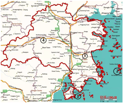
2. Wind Data in Taizhou

2.1. Reference Wind Pressure

Along the southeast coast of China, typhoon and tropical storm landfall are frequent, and the terrain is complex and mountainous. In the design of building structures, the value of the reference wind pressure has a great influence on the safety and economy of the structure. However, due to historical reasons, local weather stations with a long time history are few in number, so the reference wind pressure could not be determined only based on observation data.

In the “Load code for the design of building structures (GB50009-2012)”, only four reference wind pressures were given for Taizhou, Zhejiang Province. They were Kuocangshan in Linhai (the reference wind pressure is 0.90 kN/m²), Hongjia in Jiaojiang District (the reference wind pressure is 0.55 kN/m²), Xiadachen in Jiaojiang District (the reference wind pressure is 1.45 kN/m²), and Kanmen in Yuhuan County (the reference wind pressure is 1.20 kN/m²) (as shown in

Table 1. The reference wind pressure in the Chinese load code (GB50009-2012).

Site Name	Altitude(m)	Wind Pressure (kN/m2)
		R = 10	R = 50	R = 100
Kuocangshan	1383.1	0.60	0.90	1.05
Hongjia	1.3	0.35	0.55	0.65
Xiadachen	86.2	0.95	1.45	1.75
Kanmen	95.9	0.70	1.20	1.45

and Figure 1). The wind speed data of Xiadachen and Kanmen were collected on the island; the wind speed data of Kuocangshan were collected at the top of a mountain at an elevation of more than 1000 m above the sea level; the wind speed data of these three sites were of no reference significance to the structural design in urban areas of Taizhou. The only one that can be used for building structure design was reference wind pressure at Hongjia in Jiaojiang District. The geographical location and topography of Taizhou determine that the design wind pressure varies from countryside to the city center in Taizhou, and even from street to street in the same district. Therefore, it is of great importance to carry out CFD modeling tasks to simulate the wind velocity field associated with extreme wind events and in turn, the basic wind pressure of every county, city, district, and street in Taizhou.

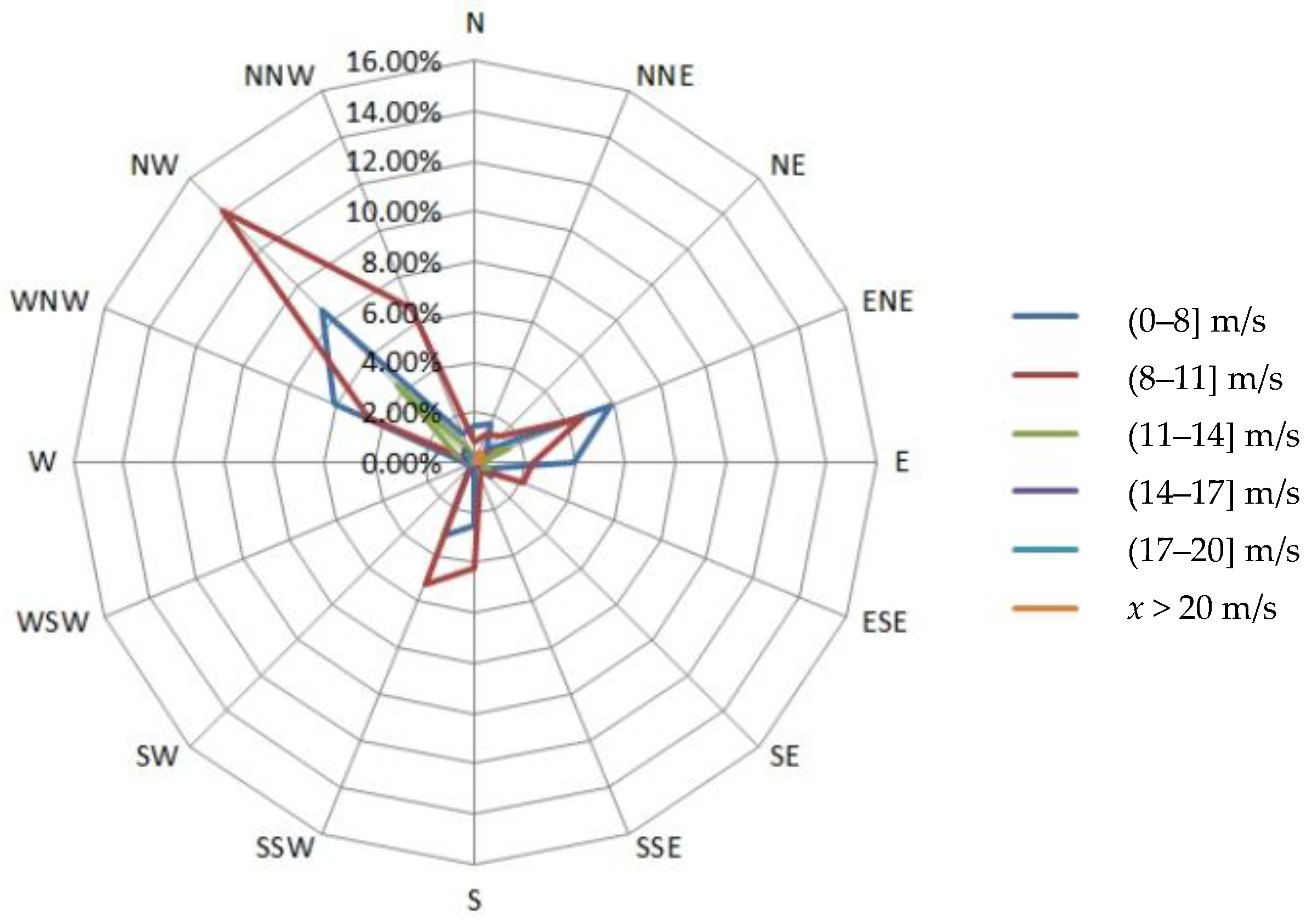
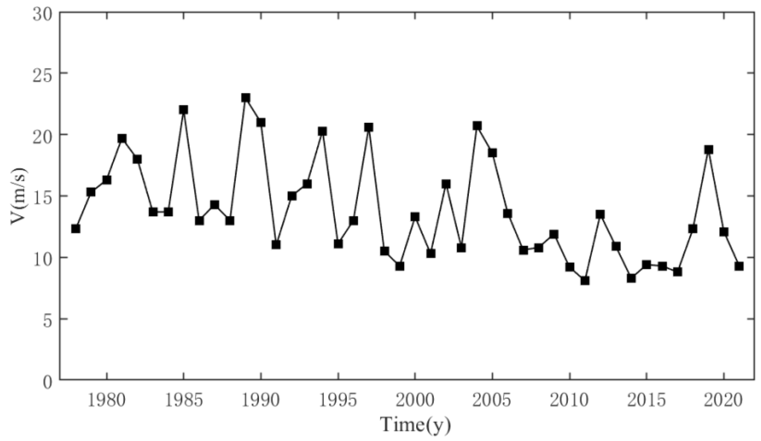
2.2. Wind Speed Data from Early Meteorological Stations

There are eight meteorological stations in Taizhou that are over 40 years old. Five of them provide valid data with complete wind data records. Since 1978, the maximum monthly wind speeds and the corresponding wind directions have been collected at five stations, as listed in

Table 2. The information of the M1 to M5 meteorological stations (referred as the five main stations).

Meteorological Station Number	M1	M2	M3	M4	M5
Meteorological station name	Tiantai	Xianju	Linhai	Wenling	Hongjia
Latitude and longitude	120°58′ E 29°09′ N	120°43′ E 28°52′ N	121°12′ E 28°52′ N	121°22′ E 28°22′ N	121°25′ E 28°37′ N
Measured maximum wind speed (m/s)	21	19	20	23.5	23
Maximum wind speed in 50-year return period (m/s)	21.53	21.69	23.74	26.40	27.22
Wind angle corresponding to maximum speed	ESE	NE	WNW	N	NNE

. The frequency of the maximum wind speed range and the frequency of the corresponding wind direction angle were counted. The wind rose diagram was plotted and graded by wind speed. Taking Hongjia weather station as an example, the frequency of occurrence in various wind directions and wind speed ranges was calculated according to the monthly extreme wind speed samples for 40 years, as reported in

Table 3. Occurrence frequency of monthly extreme wind samples in each direction and speed range (%) from 1978 to 2021 at Hongjia station.

Wind Angle	(0–5] m/s	(5–8] m/s	(8–11] m/s	(11–14] m/s	(14–17] m/s	(17–20] m/s	x > 20 m/s	Total
N	0.00	1.46	0.84	0.00	0.00	0.00	0.00	2.30
NNE	0.00	1.67	1.25	0.00	0.21	0.00	0.42	3.55
NE	0.00	0.63	1.46	0.42	0.84	0.00	0.42	3.76
ENE	0.00	5.85	4.59	1.46	0.00	0.00	0.21	12.11
E	0.00	3.97	2.30	0.21	0.00	0.00	0.21	6.68
ESE	0.00	0.63	2.09	0.63	0.00	0.00	0.00	3.34
SE	0.00	0.84	0.42	0.21	0.21	0.00	0.00	1.67
SSE	0.00	0.00	0.63	0.00	0.00	0.00	0.00	0.63
S	0.00	2.51	4.18	0.00	0.00	0.00	0.00	6.68
SSW	0.00	3.13	5.22	0.21	0.42	0.00	0.00	8.98
SW	0.00	0.21	0.21	0.00	0.00	0.00	0.00	0.42
WSW	0.00	0.21	0.00	0.00	0.00	0.21	0.00	0.42
W	0.00	0.42	0.00	0.21	0.00	0.00	0.00	0.63
WNW	0.00	6.05	4.59	0.84	0.42	0.00	0.00	11.90
NW	0.00	8.56	14.20	4.38	0.63	0.42	0.00	28.18
NNW	0.00	1.25	6.68	0.63	0.21	0.00	0.00	8.77
Total	0.00	37.37	48.64	9.19	2.92	0.63	1.25	100

. Figure 2 shows the rose diagram of the monthly extreme wind speed at Hongjia meteorological station.

As shown in Figure 3, the annual maximum wind speed series of Hongjia station was obtained based on the wind speed data from 1978–2021. From the figure, it can be seen that the annual maximum wind speed of Hongjia station over 43 years was concentrated between 10 m/s and 25 m/s. It showed an overall trend of gradually decreasing with time, which may have a relationship with the urbanization process. As urbanization has progressed, the buildings around the weather station have shown a tendency to be taller and denser, which will weaken the wind speed magnitude at that location to some extent [27]. Therefore, it can also be seen that the reference wind pressure obtained from the existing meteorological stations has reduced its significance as a guide to the wind resistance design of the actual structure.

The wind speed and direction data from these five meteorological stations are quite complete, which is very useful for studying the design wind pressure in other regions of Taizhou. There are only 95 meteorological stations in the 44 streets and 85 towns in Taizhou. Most sites were set up between 5 and 20 years ago. In the past 19 years, few typhoons have made landfall directly in Taizhou. As a result, the data of extreme wind speed collected by the stations are quite limited, and the basic wind pressure calculated by the extreme Ι probability model is also too small. It is obviously unreasonable to use these underestimated reference wind pressures for the structural design of buildings. Therefore, we proposed to use the wind speed and direction data of these five reliable meteorological stations as a reference to derive the basic wind pressure of other towns and villages in Taizhou by a meso-scale CFD simulation.

3. Numerical Simulation

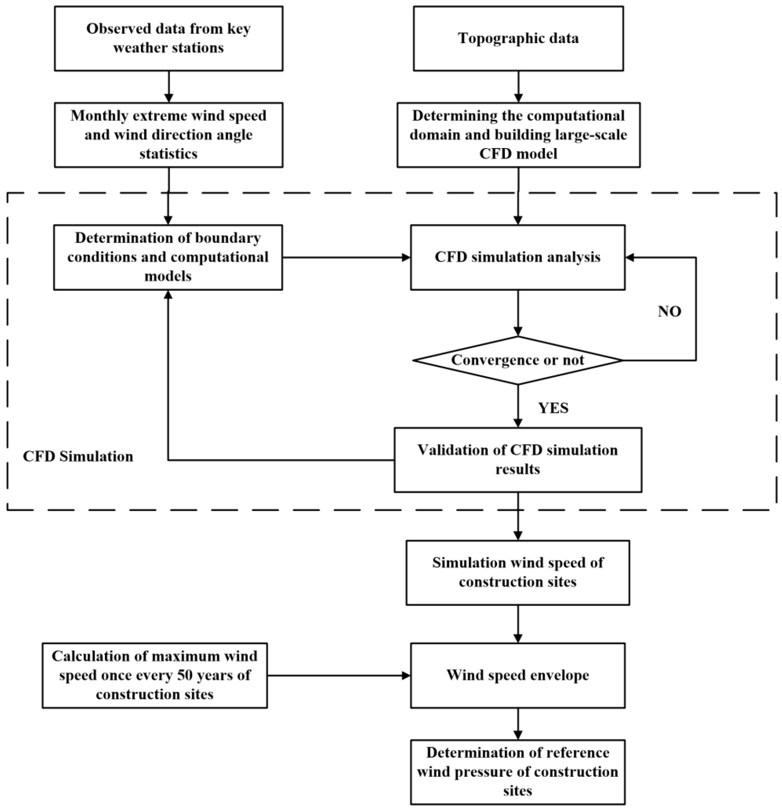
3.1. Method

Based on the ANSYS(2020) software Fluent module, a meso-scale CFD simulation was carried out to determine the reference wind pressure for selected sites in the coastal complex terrain of Taizhou. First, the computational domain would cover the whole Taizhou region (i.e., more than 10,000 km²), and a large terrain surface was established based on the topographic data of Taizhou. The maximum wind speed along the dominant wind direction was simulated. The power law was used to describe the mean wind speed profile as the inlet condition of CFD simulation. The maximum wind speed and the dominant wind direction of five main stations were taken as verification conditions for the CFD simulation results. The simulated wind speed data of each site of interest were collected. Finally, based on the simulated maximum wind speed data, the design wind speed with a 50-year return period for a site of interest was estimated according to the extreme type I probability distribution model [28]. The overall procedure to determine the design wind speed and in turn the reference wind pressure for a given site is shown in Figure 4.

3.2. Computational Domain

The terrain data were obtained from the latest geographic information of Google Map by Point-Taking (2020) software. The terrain grid was generated by interpolation with Surfer (2020) software, and the computing grid was set twice as dense as the interpolation grid. The computational domain dimension was about 150 km × 120 km × 2.57 km, as shown in Figure 5. M1 to M5 denote the locations of the five main stations. Their specific site names and wind speed parameters are shown in Table 2.

A grid sensitivity analysis was performed, and three grid schemes are shown in

Table 4. Grid sensitivity analysis schemes.

Grid Scheme	Maximum Horizontal Grid Size/m	Maximum Vertical Grid Size/m	Grid Number
Scheme 1	150	200	6.3 × 107
Scheme 2	100	100	8.1× 107
Scheme 3	50	50	1.25 × 108

. The grid sensitivity analysis shows that Scheme 2 could produce an accurate simulation with reasonable computational cost. The grid details for Scheme 2 are as follows. In the horizontal direction, the grid size was 100 × 100 m. In the vertical direction, the grid dense was gradually reduced with the increase in height. The grid size near the ground is 2 m, used for a height of 20 m; then the grid size becomes 5 m for a height of 50 m; the top grid size was 100 m with 25 layers for a height of 2500 m. The total dimension in the altitude direction was 2570 m. The total number of grids was 8.1 × 10⁷. The y+ value at the surface was in the range of 30–180, which satisfies the requirement of RANS (Reynolds averaged Navier–Stokes) simulation. The generated grids are shown in Figure 6.

3.3. Boundary Conditions and RANS

The boundary conditions mainly include several parts such as the inlet boundary, the exit boundary, the top boundary, the ground boundary, and the side boundary. The motion of the air was assumed to be an incompressible steady flow in 3D, regardless of the effect of the Coriolis effect force. For simplicity, the effect of temperature on air properties (i.e., air density) was ignored in this CFD simulation study. The dynamic viscosity coefficient of air was taken as 1.7894 × 10⁻⁵ N·S·m⁻². According to the AIJ code [7] in Japan, if the computational domain is large enough, the side and top boundary conditions have little effect on the results around the target building. The non-viscous wall state (usually the velocity component and the tangential velocity gradient are zero) and the large computational domain would make the simulation process more stable. The outlet condition was adopted as the pressure outlet.

The inlet boundary was considered as the velocity boundary condition and was set as the inlet wind velocity profile. The average wind velocity profile was described by a power law. The wind profile was determined by the formula:

$$U=U_r{(\frac{z-d}{z_r})}^a$$

(1)

where $U_r$ is the wind speed at the reference altitude $z_r$; a denotes the power law index; and d denotes the zero plane displacement. Parameters of the mean wind speed profile and boundary conditions are summarized in

Table 5. Parameters of the mean wind speed profile.

Topographic Condition	Approximate Length/m	Power Exponent a	Zero Plane Displacement d/m
Sea, mudflat, snow plain, etc.	0.000–0.003	0.1–0.13	0
Open country, open country with crops, fences, and a few trees	0.003–0.2	0.14–0.2	0.1
Dense forests, homes, suburbs	0.2–1	0.2–0.25	5
Cities	1–2	0.25–0.3	10
Big city center	2–4	0.3–0.5	10

and

Table 6. Boundary conditions.

Location	Type
Inlet	Velocity inlet
Outlet	Pressure outlet
Side surface	Symmetry
Top surface	Symmetry
Bottom surface	Wall

.

RANS (Reynolds averaged Navier–Stokes) is widely used in CFD simulation to deal with turbulence because of its high accuracy and low computational cost. The time-average momentum and continuity equations of RANS are shown as:

$$\frac{\partial \overline{u_i}}{\partial t}+\overline{u_j}\frac{\partial \overline{u_i}}{\partial x_j}=-\frac{1}{\rho }\frac{\partial \overline{p}}{\partial x_i}+\nu \frac{{\partial }^2\overline{u_i}}{\partial x_j\partial x_j}-\frac{\partial \overline{u_i^{\prime }{u}_j^{\prime }}}{\partial x_j}$$

(2)

$$\frac{\partial \overline{u_i}}{\partial x_i}=0$$

(3)

where $\overline{u_i}$ denotes the mean velocity component in Cartesian coordinates (x_j, i.e., x₁, x₂, x₃); $u_i^{\prime }$ denotes the zero-mean turbulent velocity component; $\overline{p}$ is the mean wind pressure; $\rho$ is the air density.

In the turbulence models of RANS, the k-ε turbulence model is most commonly used in the field of wind engineering. The k-ε turbulence model including the standard k-ε model, the RNG (renormalization group) k-ε model, and the realizable k-ε model. The standard k-ε model [29] was proposed by Jones and Launder, and it has particular performance in industrial engineering applications. However, the standard k-ε model produces some distortion when simulating flows with large pressure gradients, strong separation flows, strong cyclonic flows, and large curvature flows. The RNG k-ε model [30] and the realizable k-ε model [31] are the modified versions. The RNG k-ε model considers the turbulent flow in the vortex effect, adds an analytical formula for the turbulent Prandtl number, and a differential formula for the effective viscosity, which can better handle flow with a large strain rate and flow curvature. It has good performance in the field of wind engineering for hilly terrain [32].

In this work, the RNG k-ε turbulence model, as suggested in [32], was chosen for CFD simulations of the wind field over the Taizhou area. The transport equations of the RNG k-ε model are given as follows:

$$\frac{\partial k}{\partial t}+\frac{\partial \overline{k{u}_i}}{\partial x_i}=\frac{\partial }{\partial x_j}[(\nu +\frac{{\mu }_t}{{\sigma }_k})\frac{\partial k}{\partial x_j}]+P_k-\epsilon$$

(4)

$$\frac{\partial \epsilon }{\partial t}+\frac{\partial \overline{\epsilon u_i}}{\partial x_i}=\frac{\partial }{\partial x_j}[(\nu +\frac{{\mu }_t}{{\sigma }_{\epsilon RNG}})\frac{\partial \epsilon }{\partial x_j}]+\frac{\epsilon }{k}(C_{1\epsilon RNG}{P}_k-C_{2\epsilon RNG}\epsilon )$$

(5)

where $k$ is the turbulent kinetic energy and $\epsilon$ is the turbulence dissipation rate; $P_k$ represents the generation of k due to the mean velocity gradients; $\nu$ and ${\mu }_t$ are the kinematic molecular viscosity and the dynamic turbulent viscosity, respectively; ${\sigma }_k$ and ${\sigma }_{\epsilon RNG}$ are turbulent Prandtl numbers for k and ε, respectively; $C_{1\epsilon RNG}$ and $C_{2\epsilon RNG}$ denote two empirical constants in the RNG k-ε turbulence model.

The steady-state of the flow field was solved by the SIMPLE algorithm. At the same time, the residual error of each solved variable was monitored to judge whether the calculation converged or not. The numerical iteration converged when the continuous residual error was less than 0.001, or the results did not change with the increase in the iteration times.

Five cases of CFD simulation were carried out, as listed in

Table 7. The cases of CFD simulation.

Case	Reference Weather Station Name	Maximum Wind Speed in 50-Year Return Period (m/s)	Wind Angle Corresponding to Maximum Speed	Elevation of the Wind Speed Acquisition Point (m)
Case 1	Tiantai Station (M1)	21.53	ESE	108.6
Case 2	Xianju Station (M2)	21.69	NE	79.1
Case 3	Linhai Station (M3)	23.74	WNW	6.8
Case 4	Wenling Station (M4)	26.40	N	33.6
Case 5	Hongjia Station (M5)	27.22	NNE	5.3

. By adjusting the boundary inlet wind conditions, the wind speed and wind direction were solved and obtained at the five reference stations during the simulation. If the simulated wind speed and wind direction at one of five reference stations were the same as the observation result of extreme wind, the corresponding simulation case was regarded as successful. The simulated wind speed data at 44 streets and 85 towns in Taizhou was then collected from the CFD simulation case and could be used as the extreme wind speed data to determine the basic wind pressure.

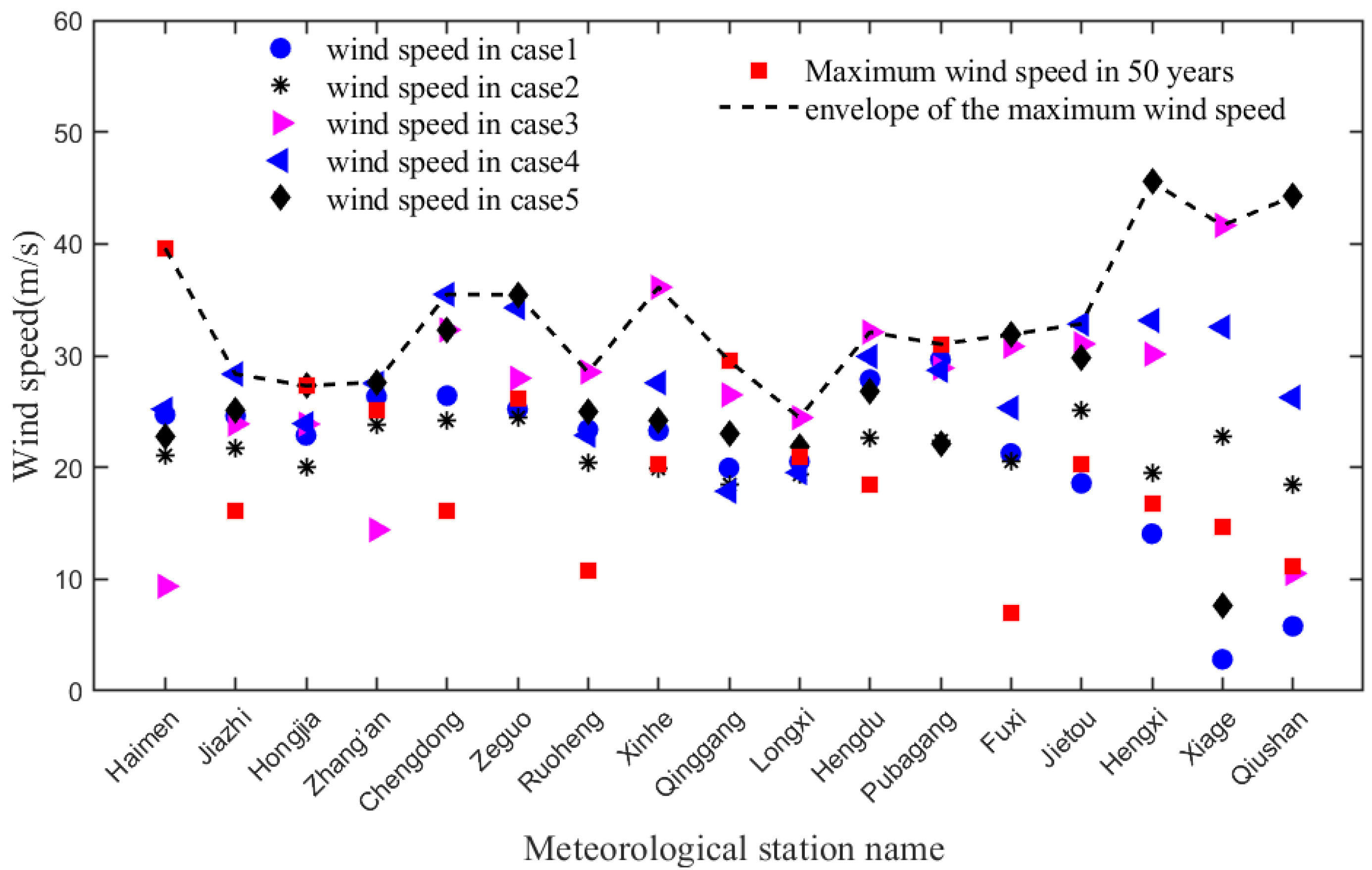
4. Results and Discussions

The simulation results of wind fields were collected at various town and street sites of Taizhou. The wind speed contour plots across the computational domain are shown for five simulation cases in Figure 7, respectively. It can be seen that the wind speed results varied from case to case. When the Tiantai, Xianju, and Linhai stations were used as the references, the maximum wind speed at the surface was about 40 m/s, while when the Wenling and Hongjia stations were used as references, the maximum wind speed could reach more than 70 m/s. Because of the large difference in elevation of the mountains in the computational domain, the uneven spatial distribution of mean wind speed was observed for each simulation case. Thus, it was necessary to carry out such a mesoscale CFD simulation study to determine the extreme wind speed and in turn the reference wind pressure for a specific site without a long history of observation data.

The wind speed and wind direction simulation data of each location (latitude, longitude and elevation) are summarized in Table 7. The 50-year return period maximum wind speeds in Table 7 were calculated according to the extreme type I probability distribution model based on the measured data collected from the five meteorological station of M1 to M5.

According to the extreme type I probability distribution model, the distribution function of extreme wind speed was:

$$F(x)=e^{-e^{[-\alpha (x-u)]}}$$

(6)

To find the extreme wind speed once in 50 years, it means the probability of x ≤ x_max is 49/50, then:

$$\exp \{-\exp [-\alpha (x-u)]\}=98\%$$

(7)

Take two natural logarithms from both sides of Equation (5) and simplify it as:

$$x_{50}=u+3.90194\frac{1}{\alpha }$$

(8)

where u and α are the position parameter and scale parameter, respectively, corresponding to the extreme type I probability distribution, which could be estimated statistically with the observed extreme wind speed data from the five main stations of M1 to M5.

A comparison of the simulated and measured wind speeds at 17 meteorological stations in Taizhou City was reported in

Table 8. Comparison of the simulated and reference wind speeds at the 17 meteorological stations in Taizhou City.

Number	Stations	Observation Duration (Year)	v50 (m/s)	Simulated Wind Speed Data (m/s)					vs (m/s)	$({\mathit{v}}_{\mathit{s}}-{\mathit{v}}_{50})/{\mathit{v}}_{50}\times 100\%$
				Case 1	Case 2	Case 3	Case 4	Case 5
1	Jiaojiang District/Haimen	19	39.62	24.71	21.01	9.37	25.2	22.77	25.2	−36.40
2	Jiaojiang District/Jiazhi	14	16.12	24.59	21.75	23.88	28.34	25.09	28.34	75.56
3	Jiaojiang District/Hongjia (M5)	51	27.27	22.87	19.98	23.87	23.91	27.30	27.30	0.11
4	Jiaojiang District/Zhang’an	19	25.13	26.34	23.75	14.41	27.52	27.62	27.62	9.83
5	Wenling City/Chengdong	14	16.17	26.41	24.16	32.3	35.47	32.34	35.47	119.54
6	Wenling City/Zeguo	19	26.14	25.21	24.44	27.97	34.28	35.44	35.44	7.12
7	Wenling City/Ruoheng	16	10.76	23.37	20.4	28.52	22.87	25.04	28.52	164.87
8	Wenling City/Xinhe	17	20.31	23.27	19.92	36.11	27.56	24.15	36.11	77.74
9	Yuhuan District/Qinggang	15	29.54	19.95	18.46	26.49	17.86	22.97	26.49	−10.33
10	Yuhuan District/Longxi	9	20.92	20.52	19.32	24.45	19.53	21.91	24.45	16.85
11	Sanmen District/Hengdu	8	18.52	27.85	22.66	32.10	29.92	26.75	32.10	73.33
12	Sanmen District/Pubagang	15	31.03	29.65	22.43	28.89	28.68	22.14	29.65	−4.46
13	Tiantai District/Fuxi	9	6.92	21.24	20.48	30.83	25.32	31.88	31.88	360.47
14	Tiantai District/Jietou	15	20.31	18.58	25.15	31.04	32.83	29.81	32.83	61.67
15	Xianju District/Hengxi	15	16.70	14.06	19.52	30.12	33.14	45.55	45.55	172.76
16	Xianju District/Xiage	9	14.71	2.83	22.80	41.65	32.56	7.67	41.65	183.03
17	Xianju District/Qiushan	7	11.15	5.79	18.41	10.51	26.26	44.24	44.24	296.69

Note: Simulated wind speed data of case 1 to case 5 were verified by stations M1 to M5, respectively; v₅₀ denotes the design wind speed of a 50-year return period estimated by statistical analysis on the observed extreme wind speed data; v_s denotes the simulated maximum wind speed in five cases.

. The difference between the simulated maximum wind speed and the 50-year return period wind speed calculated from the observation data was small for stations with a long history, but the discrepancies became large for relatively new meteorological stations with a short history. For the 51-year-old station in Hongjia (Jiaojiang district), the discrepancy between the simulation and reference wind speed was only about 0.11%. The difference between v₅₀ and v_s in Table 8 was smaller when the observation duration was more than 19 years, and the maximum was 36.4% at Haimen station. However, the difference will be larger when the observation duration of a station is less than 19 years, and the largest discrepancy of 360.47% was found at Fuxi station in Tiantai district with a 9-year observation history. Figure 8 presents a scatter plot of the simulated wind speed data for the 17 meteorological stations in Taizhou. The dotted line in the plot is the envelope of the maximum wind speed at each station.

According to the meteorological records, in the past 19 years, only in 2019 did Typhoon Lekima land in Taizhou directly. A large number of new meteorological stations have since been built with a relatively short history, but few data have been collected due to typhoon. It is difficult to estimate a reasonable 50-year return period design wind speed with the short-term observation data. This work provides an alternative mesoscale CFD simulation method to directly simulate the extreme mean wind speed with calibration to the reference design wind speed estimated from the reliable observation data of the main stations.

The wind pressure was then calculated according to the simulated maximum wind speed by Equations (9) and (10). The reference wind pressure of w₁ for a specific site could be determined as the larger one between the wind pressure from the simulation (w_s) and the estimated 50-year return period wind pressure (w₅₀). The reference wind pressure results for the 17 meteorological stations in Taizhou are summarized in

Table 9. Comparison of the simulated design wind pressure at the 17 meteorological stations in Taizhou.

Number	Station	Observation Duration (Year)	Altitude (m)	W50 (kN/m2)	ws (kN/m2)	w1 (kN/m2)
1	Jiaojiang District/Haimen	19	3	0.98	0.40	0.98
2	Jiaojiang District/Jiazhi	14	5	0.16	0.50	0.50
3	Jiaojiang District/Hongjia	51	5	0.46	0.47	0.47
4	Jiaojiang District/Zhang’an	19	5.3	0.39	0.48	0.48
5	Wenling City/Chengdong	14	185	0.16	0.77	0.77
6	Wenling City/Zeguo	19	184	0.42	0.77	0.77
7	Wenling City/Ruoheng	16	5	0.07	0.51	0.51
8	Wenling City/Xinhe	17	7	0.26	0.81	0.81
9	Yuhuan District/Qinggang	15	18	0.54	0.44	0.54
10	Yuhuan District/Longxi	9	48	0.27	0.37	0.37
11	Sanmen District/Hengdu	8	52	0.21	0.64	0.64
12	Sanmen District/Pubagang	15	15	0.60	0.55	0.60
13	Tiantai District/Fuxi	9	52	0.03	0.63	0.63
14	Tiantai District/Jietou	15	113	0.25	0.67	0.67
15	Xianju District/Hengxi	15	116	0.17	1.28	1.28
16	Xianju District/Xiage	9	142	0.13	1.07	1.07
17	Xianju District/Qiushan	7	150	0.08	1.21	1.21

.

$$w=\frac{1}{2}\rho v^2$$

(9)

where v is the 50-year return period mean extreme wind speed, and the air density can be calculated as:

$$\rho =0.00125e^{-0.0001z}$$

(10)

where z is the altitude of the observation station.

It can be seen from Table 9 that the reference wind pressure of the four stations in Jiaojiang District was calculated to be around 0.5 kN/m². The locations of these four Jiaojiang stations are close to the same natural environment. Therefore, the estimated reference wind pressures of four Jiaojiang stations were all close to the 0.55 kN/m² given in the Chinese code [33]. The reference wind pressures for stations in Wenling ranged from 0.39 kN/m² to 0.81 kN/m² based on the simulated mean extreme wind speed of each case. Since the reference wind pressure in Wenling is not specified in the Chinese code, the reference wind pressure obtained in this work could be used for the wind-resistant structural design of buildings in Wenling.

Based on this work, the CFD simulation data of the mean extreme wind speed of 44 streets and 85 towns in Taizhou were gathered, and the reference wind pressure for building design was calculated.

5. Conclusions

This paper presents a mesoscale CFD simulation framework to determine the reference wind pressure of sites in a complex terrain where few extreme wind speed data are available. The framework was successfully applied to investigate the wind field over the whole region of Taizhou City by establishing a mesoscale CFD model and conducting turbulence simulation. The estimated 50-year design wind speed from five reliable main stations of Taizhou was used in CFD simulation as the validation conditions. The reference wind pressure was calculated from the simulated extreme wind speed and verified for sites with a long history of meteorological records. The simulated extreme wind speed for sites without a long history of meteorological records could then be used to determine the reference wind pressure, which is the critical parameter for the wind-resistant structural design of buildings. The 50-year return period reference wind pressure results produced by this work has been adopted for practical building design in Taizhou. The novel approach developed in this study provides an effective and alternative means for the determination of the design wind pressure in sites of a complex terrain without a long history of meteorological records.

References

1. Cravero, C.; Leutcha, P.J.; Marsano, D. Simulation and Modeling of Ported Shroud Effects on Radial Compressor Stage Stability Limits. Energy 2022, 15, 2571. [Google Scholar] [CrossRef]
2. Hargreaves, D.M.; Wright, N.G. On the use of the k–ε model in commercial CFD software to model the neutral atmospheric boundary layer. J. Wind Eng. Ind. Aerod. 2007, 95, 355–369. [Google Scholar] [CrossRef]
3. Tamura, Y.; Ohkuma, T.; Kawai, H.; Uematsu, Y.; Kondo, K. Revision of AIJ Recommendations for Wind Loads on Buildings. In Structures 2004: Building on the Past, Securing the Future 2004; ASCE: Reston, VA, USA, 2004; pp. 1–10. [Google Scholar]
4. Wright, N.G.; Easom, G.J. Comparison of several computational turbulence models with full-scale measurements of flow around a building. Wind Struct. 1999, 2, 305–323. [Google Scholar] [CrossRef]
5. Ricci, A.; Kalkman, I.; Blocken, B.; Burlando, M.; Repetto, M.P. Impact of turbulence models and roughness height in 3D steady RANS simulations of wind flow in an urban environment. Build. Environ. 2020, 171, 106617. [Google Scholar] [CrossRef]
6. Schneider, S.; Santhanavanich, T.; Koukofikis, A.; Coors, V. Exploring schemes for visualizing urban wind fields based on CFD simulations by employing OGC standards. In Proceedings of the ISPRS Annals of the Photogrammetry, Remote Sensing and Spatial Information Sciences, Virtual, 31 August–2 September 2020; Copernicus GmbH: Strasbourg, France, 2020. [Google Scholar]
7. Tominaga, Y.; Mochida, A.; Yoshie, R.; Kataoka, H.; Nozu, T.; Yoshikawa, M.; Shirasawa, T. AIJ guidelines for practical applications of CFD to pedestrian wind environment around buildings. J. Wind Eng. Ind. Aerod. 2008, 96, 1749–1761. [Google Scholar] [CrossRef]
8. Mochida, A.; Tominaga, Y.; Murakami, S.; Yoshie, R.; Ooka, R. Comparison of various k-εmodels and DSM applied to flow around a high-rise building: Report on AIJ cooperative project for CFD prediction of wind environment. Wind Struct. Int. J. 2002, 5, 227–244. [Google Scholar] [CrossRef] [Green Version]
9. Ferziger, J.H.; Perić, M.; Street, R.L. Computational Methods for Fluid Dynamics; Springer: Berlin/Heidelberg, Germany, 2002. [Google Scholar]
10. Guideline, V. Environmental Meteorology–Prognostic Micro-scale Wind Field Models–Evaluation for Flow Around Buildings and Obstacles; Beuth Verlag GmbH: Berlin, Germany, 2005. [Google Scholar]
11. Verein, D.I. Environmental Meteorology, Physical Modelling of Flow and Dispersion Processes in the Atmospheric Boundary Layer, Application of Wind Tunnels; Verein Deutcher Ingenier: Dusserdorf, Germany, 2000. [Google Scholar]
12. Hall, R.C. Evaluation of Modelling Uncertainty-CFD Modelling of Nearfield Atmospheric Dispersion; EU Project EV5V-CT94-0531, Final Report; WS Atkins Consultants Ltd.: Epsom, UK, 1997. [Google Scholar]
13. Li, S.H.; Sun, X.J.; Zhang, S.; Zhao, S.J.; Zhang, R.W. A Study on Microscale Wind Simulations with a Coupled WRF-CFD Model in the Chongli Mountain Region of Hebei Province, China. Atmosphere 2019, 10, 731. [Google Scholar] [CrossRef] [Green Version]
14. Huang, M.F.; Sun, J.P.; Wang, Y.F.; Lou, W.J. Multi-scale simulation of typhoon wind fields by coupling of weather research and forcasting model and large-eddy simulation. J. Build. Struct. 2020, 41, 63–70. (In Chinese) [Google Scholar]
15. Hosseinzadeh, A.; Keshmiri, A. Computational Simulation of Wind Microclimate in Complex Urban Models and Mitigation Using Trees. Buildings 2021, 11, 112. [Google Scholar] [CrossRef]
16. Li, M.X.; Qiu, X.F.; Shen, J.J.; Xu, J.Q.; Feng, B.; He, Y.J.; Shi, G.P.; Zhu, X.C. CFD Simulation of the Wind Field in Jinjiang City Using a Building Data Generalization Method. Atmosphere 2019, 10, 326. [Google Scholar] [CrossRef] [Green Version]
17. Chang, S.Z.; Jiang, Q.G.; Zhao, Y. Integrating CFD and GIS into the Development of Urban Ventilation Corridors: A Case Study in Changchun City, China. Sustainability 2018, 10, 1814. [Google Scholar] [CrossRef]
18. Peng, L.; Liu, J.P.; Wang, Y.; Chan, P.W.; Lee, T.C.; Peng, F.; Wong, M.S.; Li, Y.G. Wind weakening in a dense high-rise city due to over nearly five decades of urbanization. Build. Environ. 2018, 138, 207–220. [Google Scholar] [CrossRef]
19. Wang, Q.; Luo, K.; Yuan, R.Y.; Wang, S.; Fan, J.R.; Cen, K.F. A multiscale numerical framework coupled with control strategies for simulating a wind farm in complex terrain. Energy 2020, 203, 117913. [Google Scholar] [CrossRef]
20. Duran, P.; Meissner, C.; Casso, P. A new meso-microscale coupled modelling framework for wind resource assessment: A validation study. Renew. Energy 2020, 160, 538–554. [Google Scholar] [CrossRef]
21. Antonini, E.; Romero, D.A.; Amon, C.H. Optimal design of wind farms in complex terrains using computational fluid dynamics and adjoint methods. Appl. Energy 2020, 261, 114426. [Google Scholar] [CrossRef]
22. Keck, R.E.; Sondell, N. Validation of uncertainty reduction by using multiple transfer locations for WRF-CFD coupling in numerical wind energy assessments. Wind Energy Sci. 2020, 5, 997–1005. [Google Scholar] [CrossRef]
23. Kuo, J.; Rehman, D.; Romero, D.A.; Amon, C.H. A novel wake model for wind farm design on complex terrains. J. Wind Eng. Ind. Aerod. 2018, 174, 94–102. [Google Scholar] [CrossRef]
24. Dhunny, A.Z.; Lollchund, M.R.; Rughooputh, S. Wind energy evaluation for a highly complex terrain using Computational Fluid Dynamics (CFD). Renew. Energy 2017, 101, 1–9. [Google Scholar] [CrossRef]
25. Ke, S.T.; Zhu, R.K. Typhoon-Induced Wind Pressure Characteristics on Large Terminal Roof Based on Mesoscale and Microscale Coupling. J. Aerosp. Eng. 2019, 32, 04019093. [Google Scholar] [CrossRef]
26. Huang, W.F.; Zhou, T.; Chen, X. Wind environment assessment of typical building groups by using CFD numerical simulation. J. Hefei Univ. Technol. (Nat. Sci. Ed.) (China) 2019, 42, 415–421. [Google Scholar]
27. Huang, M.F.; Li, Q.; Xu, H.W.; Lou, W.J.; Lin, N. Non-stationary statistical modeling of extreme wind speed series with exposure correction. Wind Struct. 2018, 26, 129–146. [Google Scholar]
28. Huang, M.F.; Li, Q.; Chan, C.M.; Lou, W.J.; Kwok, K.; Li, G. Performance-based design optimization of tall concrete framed structures subject to wind excitations. J. Wind Eng. Ind. Aerod. 2015, 139, 70–81. [Google Scholar] [CrossRef]
29. Jones, W.P.; Launder, B.E. The prediction of laminarization with a two-equation model of turbulence. Int. J. Heat Mass Tran. 1972, 15, 301–314. [Google Scholar] [CrossRef]
30. Yakhot, V.; Orszag, S.A. Renormalization group analysis of turbulence. I. Basic theory. J. Sci. Comput. 1986, 1, 3–51. [Google Scholar] [CrossRef]
31. Shih, T.; Liou, W.W.; Shabbir, A.; Yang, Z.; Zhu, J. A new k-ϵ eddy viscosity model for high reynolds number turbulent flows. Comput. Fluids 1995, 24, 227–238. [Google Scholar] [CrossRef]
32. Kim, H.G.; Patel, V.C.; Lee, C.M. Numerical simulation of wind flow over hilly terrain. J. Wind Eng. Ind. Aerod. 2000, 87, 45–60. [Google Scholar] [CrossRef]
33. Ministry of Housing and Urban-Rural Development of the People’s Republic of China. Load Code for the Design of Building Structures (GB 50009-2012); China Architecture and Building Press: Beijing, China, 2012. (In Chinese) [Google Scholar]
Figure 1. The reference wind pressure sites for Taizhou in the Load code for the design of building structures (GB50009-2012). Note: The circled numbers are the locations with a specified reference wind pressure in GB50009-2012. ➀—Hongjia; ➁—Xiadachen; ➂—Kanmen; ➃—Kuocangshan.
Applsci 12 10481 g001
Figure 2. Monthly extreme wind rises at Hongjia station from 1978 to 2021.
Applsci 12 10481 g002
Figure 3. Annual maximum wind speed series of Hongjia station from 1978 to 2021.
Applsci 12 10481 g003
Figure 4. The overall procedure to determine the reference wind pressure.
Applsci 12 10481 g004
Figure 5. Computational domain of the CFD model (m).
Applsci 12 10481 g005
Figure 6. Computational grids of the CFD model.
Applsci 12 10481 g006
Figure 7. Wind speed contour map plots of five simulation cases: (a) Case 1; (b) Case 2; (c) Case 3; (d) Case 4; (e) Case 5.
Applsci 12 10481 g007aApplsci 12 10481 g007b
Figure 8. Maximum wind speed results and their envelope for the 17 meteorological stations in Taizhou City.
Applsci 12 10481 g008