Improving Air Pollution Prediction System through Multimodal Deep Learning Model Optimization

Abstract

Many forms of air pollution increase as science and technology rapidly advance. In particular, fine dust harms the human body, causing or worsening heart and lung-related diseases. In this study, the level of fine dust in Seoul after 8 h is predicted to prevent health damage in advance. We construct a dataset by combining two modalities (i.e., numerical and image data) for accurate prediction. In addition, we propose a multimodal deep learning model combining a Long Short Term Memory (LSTM) and Convolutional Neural Network (CNN). An LSTM AutoEncoder is chosen as a model for numerical time series data processing and basic CNN. A Visual Geometry Group Neural Network (VGGNet) (VGG16, VGG19) is also chosen as a CNN model for image processing to compare performance differences according to network depth. The VGGNet is a standard deep CNN architecture with multiple layers. Our multimodal deep learning model using two modalities (i.e., numerical and image data) showed better performance than a single deep learning model using only one modality (numerical data). Specifically, the performance improved up to 14.16% when the VGG19 model, which has a deeper network, was used rather than the VGG16 model.

1. Introduction

As science and technology advance daily, the quality of life has improved, but air pollution is also increasing in various forms. Fine dust causes or worsens symptoms, such as heart- and lung-related diseases [1]. Among many studies on air pollution, studies on predicting fine dust have been conducted using prediction models of time series data to prevent such health damage. However, most studies include various types of data (e.g., PM₁₀, temperature, dew point, and wind speed) but do not include aerosol data. Aerosol refers to fine substances floating in the atmosphere, including fine dust, and it is useful for predicting fine dust movement and accumulation because of atmospheric diffusion.

In this paper, the numerical dataset that demonstrated the best performance among the datasets constructed in the previous study [2] was referred to, and the aerosol image data highly related to fine dust was added to enhance the model’s performance. However, the preconfigured numerical data was in units of hour, so the multimodal dataset was constructed by adding a satellite image with information on aerosol particle size, which was organized by the hour to match this. In addition, the satellite image contains aerosol data of the entire Korean Peninsula, so the overall flow of fine dust on the Korean Peninsula can be observed.

In this paper, we propose a multimodal deep learning model by combining the Long Short Term Memory (LSTM) series model that shows superior performance in time series data prediction and the Convolutional Neural Network (CNN) series models useful for image processing to learn the configured dataset. The multimodal deep learning model suggested in this paper combines the features of the numerical and image datasets processed by the CNN series model, so it is necessary to process many features. Therefore, the LSTM series model used the LSTM AutoEncoder, which had the best performance when there were many features. In the previous study [2], the CNN series model used a basic CNN and VGGNet (VGG16, VGG19) to compare the performance difference according to network depth. The VGGNet model is a standard deep CNN architecture with multiple layers, developed by the Visual Geometry Group, a research team at Oxford University.

As a result, the multimodal deep learning models using numerical and image data performed better than the LSTM series model using only numerical data. Among them, the performance was the best when using VGG19, which has the deepest network depth among the CNN series models. In addition, we divided the image data into original and cropped images and applied each to a multimodal deep learning model to compare the performance difference. To maximize the model’s performance, the hyperparameter set in the model was optimized using katib, a hyperparameter optimization system. The contents mentioned above are described in detail below.

The paper is composed as follows. Section 2 describes related research, and Section 3 presents the constructed dataset. Next, Section 4 defines the proposed model for the dataset, and Section 5 explains the hyperparameter optimization of the configured model. Section 6 describes the experiment and ends with the conclusion and future work in Section 7.

2. Related Research

Various time series prediction models for weather forecasting have been studied. Athira [3] utilized deep learning models using AirNet, which is pollution and weather time series data for future PM₁₀ predictions. In this study, RNN, LSTM, and GRU were used for time series data learning, and GRU performed best because only part of AirNet was used due to resource problems.

Chau [4] suggested deep learning-based Weather Normalized Models (WNM) to quantify air quality changes during the partial shutdown period due to the COVID-19 pandemic in Quito, Ecuador. Deep learning algorithms used CNN, LSTM, RNN, Bi-RNN, and GRU, among which WNM using LSTM and Bi-RNN performed the best.

Moreover, Salman [5] presented an LSTM model that adds intermediate variable signals to LSTM memory blocks to predict the weather in the Indonesian airport region and explores various architectures such as single- and multilayer LSTM. The proposed model showed that the intermediate variable could enhance the model’s predictive ability. The best LSTM model and intermediate data were the multilayer LSTM model and pressure variable, respectively.

Bekkar [6] proposed a hybrid model based on CNN and LSTM to predict PM_2.5 per hour in Beijing, China. Based on the hybrid model, we use CNN to extract spatial and internal properties for input values and apply time series data for extracted values using LSTM. The suggested model performed better than the existing deep learning models (i.e., LSTM, Bi-LSTM, GRU, and Bi-GRU).

The studies mentioned earlier use time series prediction models, such as RNN, LSTM, and GRU, similar to our research but do not use multimodal data in contrast to our approach.

Few works adopt multimodal data for weather forecasting prediction performance. Xie [7] presented a multimodal deep learning model that combines CNN and GRU to perform PM_2.5 predictions in the Wuxi region over 6 h based on data provided by the Wuxi environmental protection agency. The CNN utilizes a one-dimensional convolution layer, which extracts and integrates local variation trends and spatial correlation characteristics of multimodal air quality data. A GRU learns long-term dependencies based on the CNN results. The proposed model performed better than the existing single deep learning model (i.e., Shallow Neural Network, LSTM, and GRU). Kalajdjieski [8] recommended a custom pretrained inception model to estimate (i.e., classify whether images collected with observations are contaminated) by air pollution in the Skopje region in northern Macedonia using multimodal data composed of weather data retrieved via sensors and image data from Skopje using cameras. The proposed model is a structure that adds a new sub-model path to the pretrained inception model that processes image data, receives weather data as input, and connects the result of three fully connected layers and the output processed by the pretrained inception model to the fully connected layer again. It performed better than existing models (e.g., CNN, ResNet, and pretrained inception).

Our research differs from Xie’s [7] and Kalajdjieski’s [8] work. While the multimodal data in Xie [7] are both numerical, we use image and numerical data, such as SO₂, PM₁₀, and wind speed, from various regions. Kalajdjieski’s work aims to classify images into polluted or unpolluted, utilizing sensory weather data (e.g., temperature). Unlike Kalajdjieski’s study, our goal is to predict future PM₁₀ based on the satellite image and numerical weather data.

This paper configured multimodal data by adding image data because the image data has information on aerosol particle size. Aerosol can determine the possibility of fine dust movement and accumulation due to atmospheric diffusion, which helps predict fine dust. Thus, we tried to increase performance by constructing multimodal data with numerical and image data that affect fine dust.

3. Dataset

In our previous work [2], we forecast fine dust after 8 h using only numerical data, and the best performance was obtained when up to 5 h prior data were used as an input value. In this paper, we construct a multimodal dataset by merging satellite image data with the same numerical dataset in [2] to improve performance further.

3.1. Numerical Dataset

In our previous study [2], we constructed various datasets by merging the Korea Meteorological Administration (KMA) data providing information, such as temperature, precipitation, wind speed, and AirKorea data providing information on air pollutants.

In this paper, we adopted the features that showed the best performance in the previous study [2]. Our weather data collecting sites span seven regions of metropolitan cities (e.g., Busan and Incheon) and administrative regions (e.g., Gyeonggi-do, Chungcheongbuk-do, and Gangwon-do). Both the satellite image and the numerical data are collected for 2020. The seven regions above metropolitan cities and administrative districts have multiple weather data collecting sites (e.g., 15 in Busan, 17 in Incheon, 7 in Chungcheongbuk-do, and 4 in Gangwon-do). Each site has five features (e.g., SO₂, NO₂, CO, O₃, and PM₁₀). We selected sites in each region with a large population. The reason for the fine dust generation is the combustion of fossil fuels (e.g., coal and petroleum) due to electronic products, such as gas stoves and vacuum cleaners used at home, exhaust gas from cars, and smoke. The larger the population, the more factors cause fine dust. In addition, “month” was added as a feature to reflect the characteristics of the season, and the west sea wind direction of Incheon was included because the Korean Peninsula was affected by fine dust caused by the westerly wind.

However, in the process of composing a new dataset by referring to the dataset used in the previous study [2], there were sites with no measuring stations from 2020. We excluded those sites in the new multimodal dataset for the year 2020, and the total number of features in the dataset in this study is 1030, and the number of sample is 8784.

3.2. Satellite Image Dataset

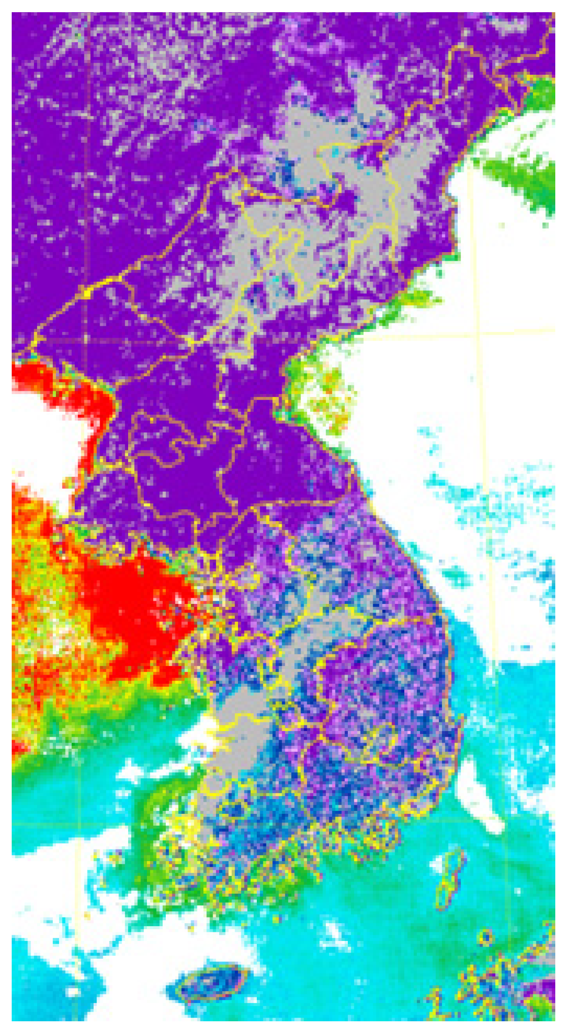
In this paper, aerosol data [9] was employed for predicting fine dust because it can determine the movement and accumulation according to atmospheric diffusion. Therefore, we constructed a multimodal dataset composed of numerical data and hourly satellite images with aerosol particle size information. The satellite image contains aerosol data for the entire Korean Peninsula so that you can see the overall flow of fine dust on the Korean Peninsula. The aerosol image data after November 2019 are provided at the National Meteorological Satellite Center.

Figure 1 shows an example of a satellite image with aerosol particle size color legend on the bottom right corner. Aerosol particle size is expressed as α. Particle size is exponential using the ratio of the two wavelengths to the corresponding optical thickness, and the range of α is −0.5–3 [10]. In Figure 1, it can be seen that the colors are different depending on the calculation range of α, and the purple series (α: −0.5–0) and the blue series (α: 0–1) represent large aerosols such as yellow dust and sea salt particles. The green series (α: 1–2) denote medium-sized aerosols, and the yellow and red (α: 2–3) correspond to fine aerosols, such as pollutants or smoke. That is, the smaller the production range of α, the larger the size of the aerosol particle, and the greater the production range of α, the smaller the size of the aerosol particle.

3.3. Cropped Satellite Image Dataset

Cropping means the act of removing unwanted areas from an image. Figure 1 presents aerosol data for Korea and other countries. However, the rest of the area in the satellite image is removed since the numerical data constructed is only for the Korean Peninsula, as shown in Figure 2. We later show how the prediction performance varies depending on the satellite image datasets. We later show how the prediction performance varies depending on the satellite image datasets.

4. Deep Learning Models

In this paper, we construct multimodal deep learning models based on the LSTM and CNN models. The LSTM is a well-known deep learning model for time series data, and the CNN is a recognized model for image data. We combine those two models for our multimodal deep learning model, handling numerical and image data.

4.1. LSTM AutoEncoder

The LSTM [11] model solves the problem related to information from the past cannot be transmitted up to the end in a long time series structure, which is a disadvantage of RNN [11]. The LSTM model has many variants, such as bidirectional-LSTM.

The multimodal deep learning model proposed in this paper combines the features of the numerical dataset, which are processed by the LSTM-based model, with the features of the image dataset, processed by the CNN-based model. As a result, the number of features increases, making learning difficult due to increased dimensions. To solve this problem, we use the LSTM AutoEncoder that efficiently encodes the high-dimensional data. We already showed that LSTM AutoEncoder outperforms the vanilla LSTM model in our problem [2].

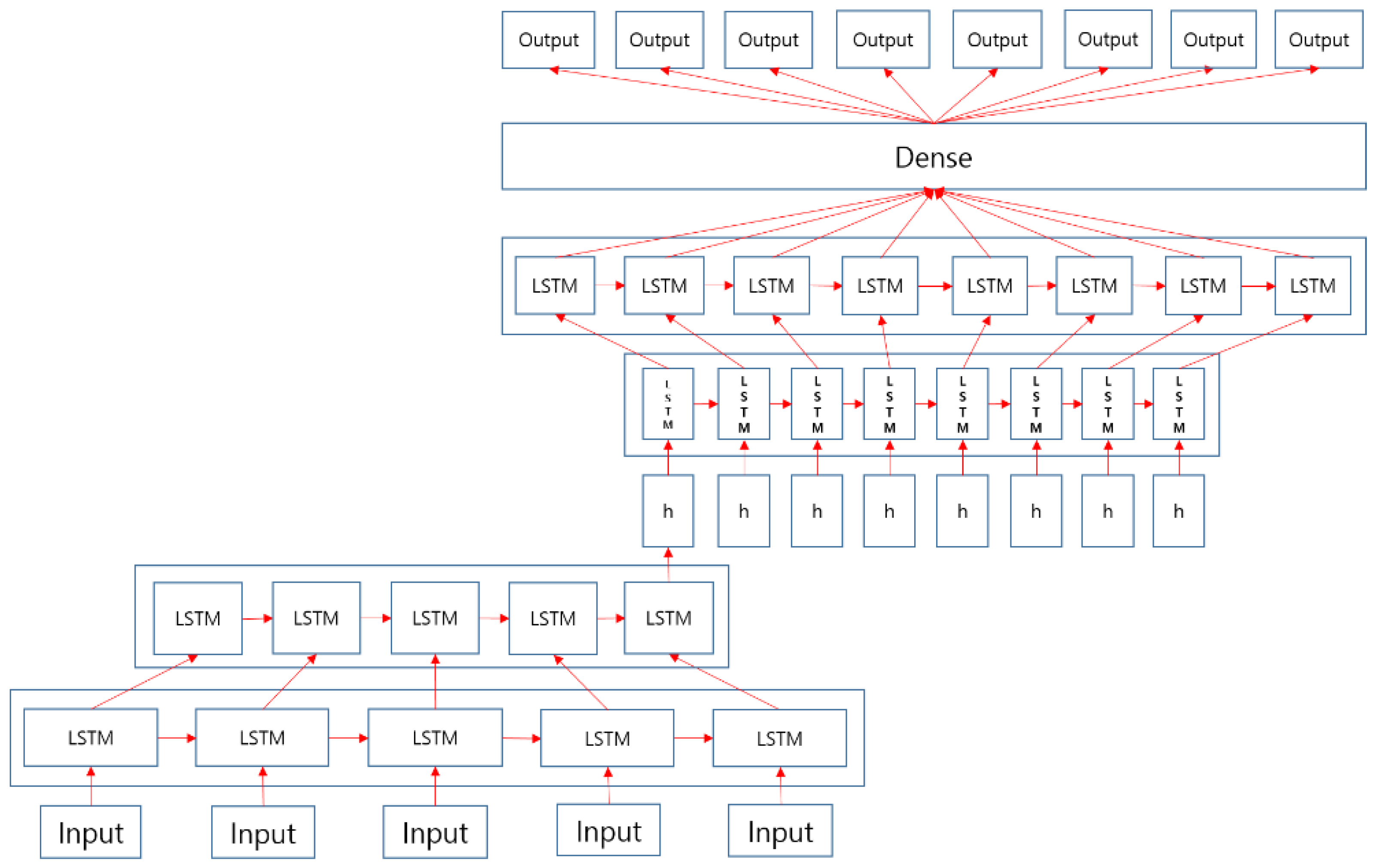
The LSTM AutoEncoder has a layer on top of LSTM layers to extract features by reducing input data dimension [12] and creating original data based on the extracted features. In general, the AutoEncoder is widely used for self-supervised learning or unsupervised learning, where the input and the label are the same, but in our previous work [2], the AutoEncoder is used for supervised learning. Figure 3 shows the LSTM AutoEncoder implemented in our previous work [2], where the encoder has two LSTM layers for input and dimensionality reduction, and the decoder also has two LSTM layers for output and dimensionality recovery. The original input value of the constructed model, data from the past 5 h, goes through the encoder and decoder to predict PM₁₀ values after 1–8 h from the present.

4.2. Basic CNN (Convolutional Neural Networks)

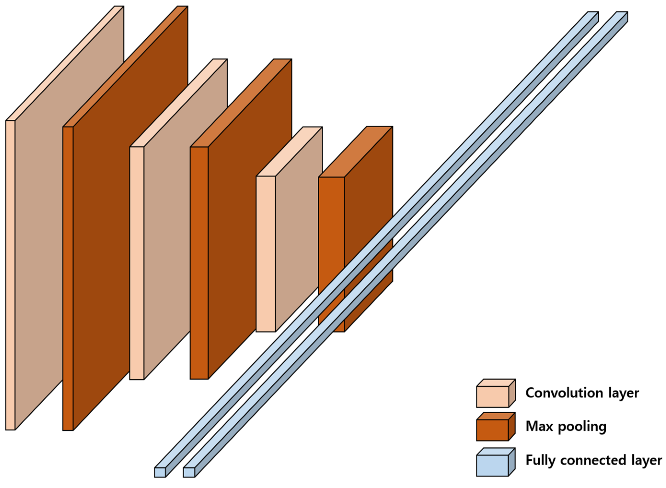
We first use the basic CNN [13] to handle satellite images to compare the performance of sophisticated CNN models, such as VGGNet. The CNN model solves the problem of common neural network inputs without spatial/topological information and determines the association between each pixel of the image and the surrounding pixels by processing it in part rather than the entire image. In this way, the CNN can learn images while maintaining spatial information of the images. Thus, it is widely used for image processing, and the feature of the image is extracted through convolution layers and pooling layers. The basic CNN experimented with in this paper is shown in Figure 4 and has a total of 5 layers consisting of 3 convolution/pooling layers and 2 fully connected layers.

4.3. VGGNet

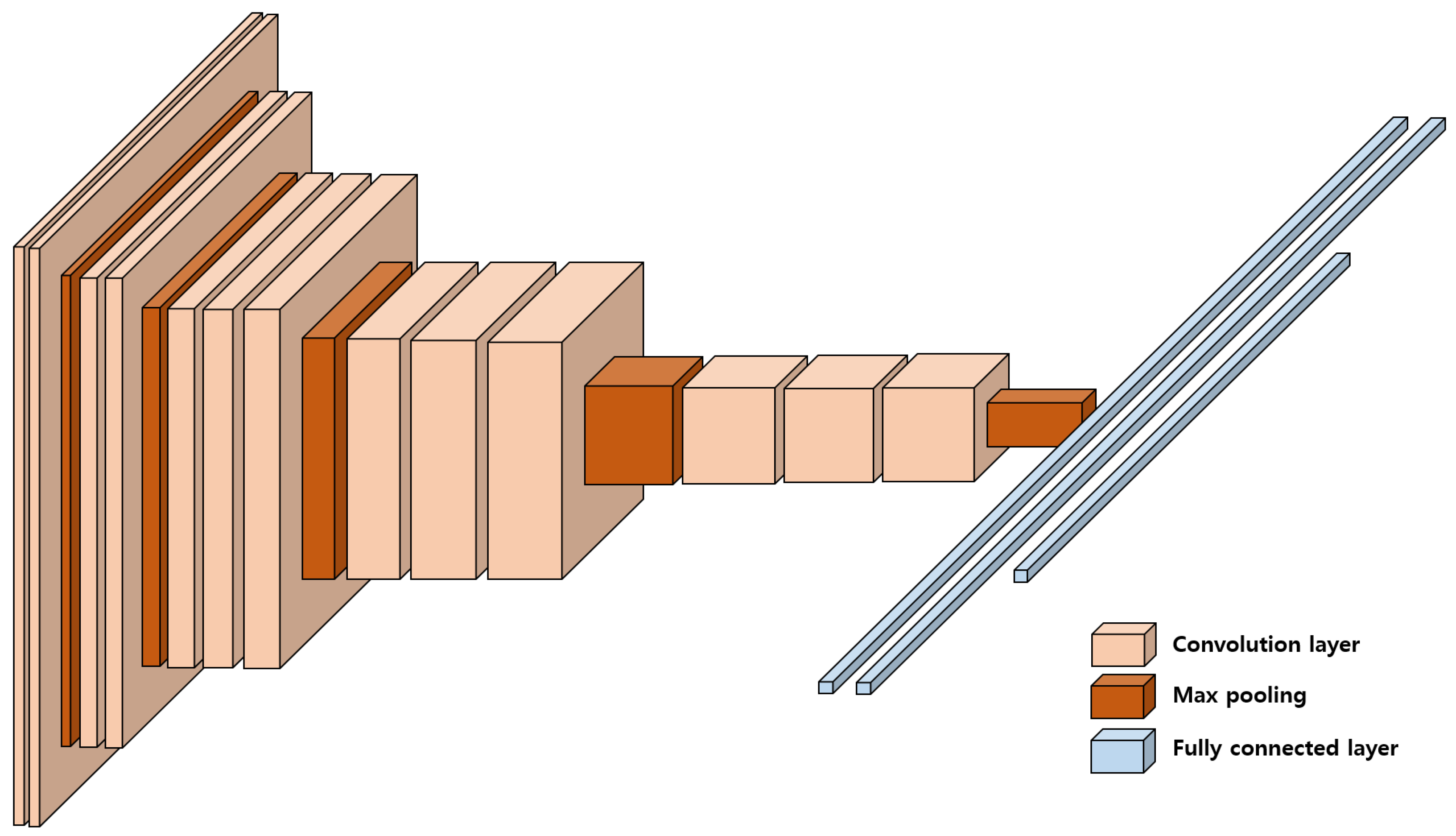
We conducted experiments with the VGGNet model [14] as a sophisticated CNN model in contrast to the basic CNN model to compare the effectiveness of various CNN models. The VGGNet is a CNN series model developed by the Visual Geometry Group, a research team at Oxford University. It is a standard deep CNN architecture with multiple layers. We chose the VGGNet model because other models, such as the ResNet deeper than VGGNet, require more time and memory during training, resulting in practical difficulties in experiments. The VGGNet model is deeper than the basic CNN model, and the filter size is fixed as small as 3 × 3. The idea of VGGNet is to use multiple convolution layers consisting of small-sized 3 × 3 filters instead of a convolution layer consisting of large-sized filters. As a result, the number of parameters is reduced, which is efficient in terms of computational amount and increases the training speed. Furthermore, as the depth of the model deepens, the performance is improved because it can express high-dimensional nonlinearity. According to the number of layers, VGGNet is called VGG16 (Figure 5) if it has 16 layers (13 convolution layers + 3 fully connected layers) and VGG19 if it has 19 layers (16 convolution layers + 3 fully connected layers). The VGG research team made a total of six structures (A (11), A-LRN (11), B (13), C (16), D (16) and E (19)) and compared their performance to check the performance difference according to depth. As a result, it was confirmed that the performance improved as the depth increased from 11, 13, 16, to 19 layers. VGGNet is used to process satellite images and, in this paper, VGG16 and VGG19.

4.4. Multimodal Deep Learning

Multimodal refers to utilizing two or more modalities, including text and image/text and sound/numerical data and image. The process of constructing and learning a deep learning model is called multimodal deep learning [15]. Multimodal deep learning allows us to correlate relationships between different modalities and solve various problems. In this paper, we construct a multimodal deep learning model for learning different data relationships according to time series characteristics through numerical and image data. However, since numerical and image data have different characteristics, we need to integrate these data.

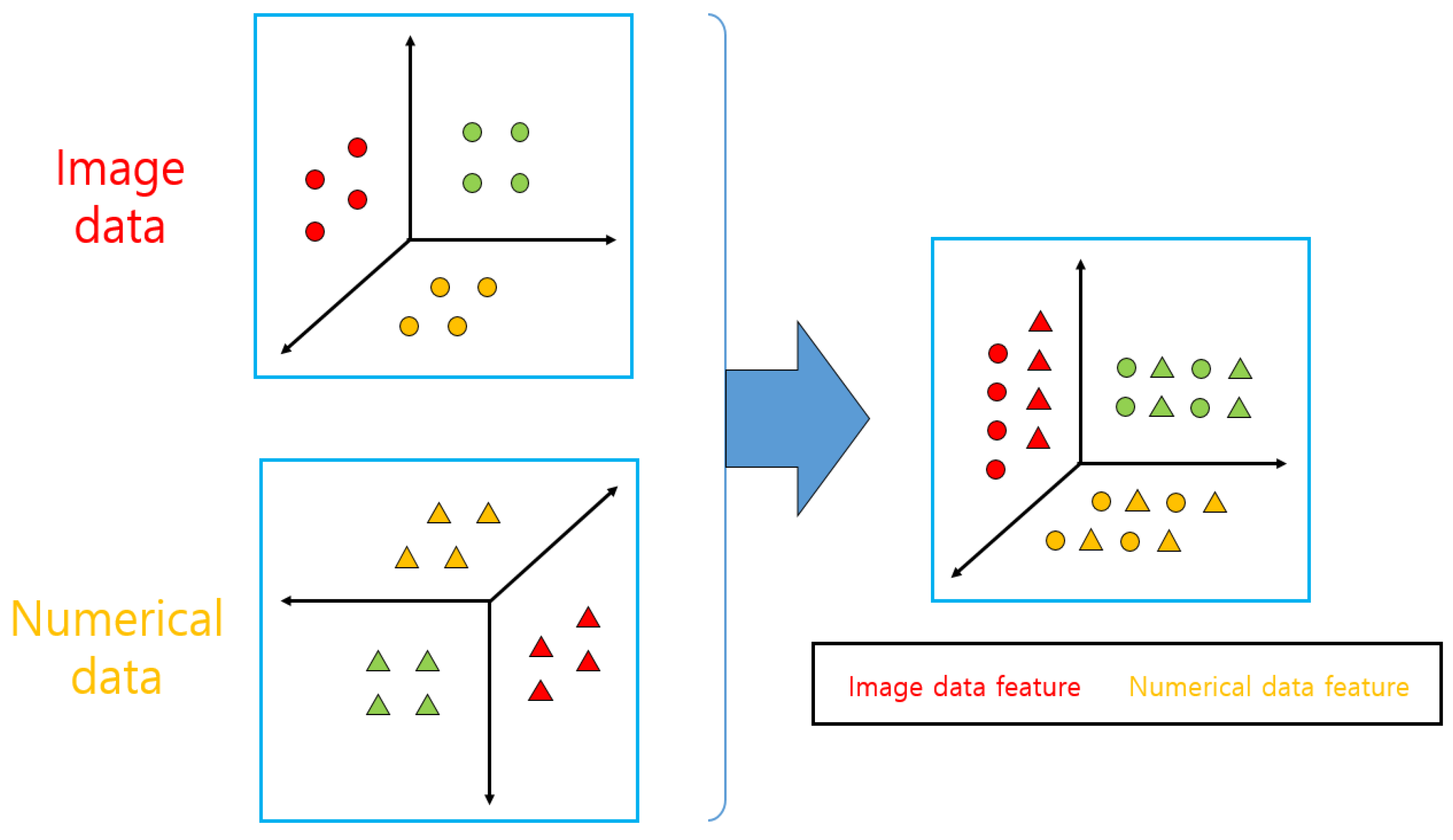
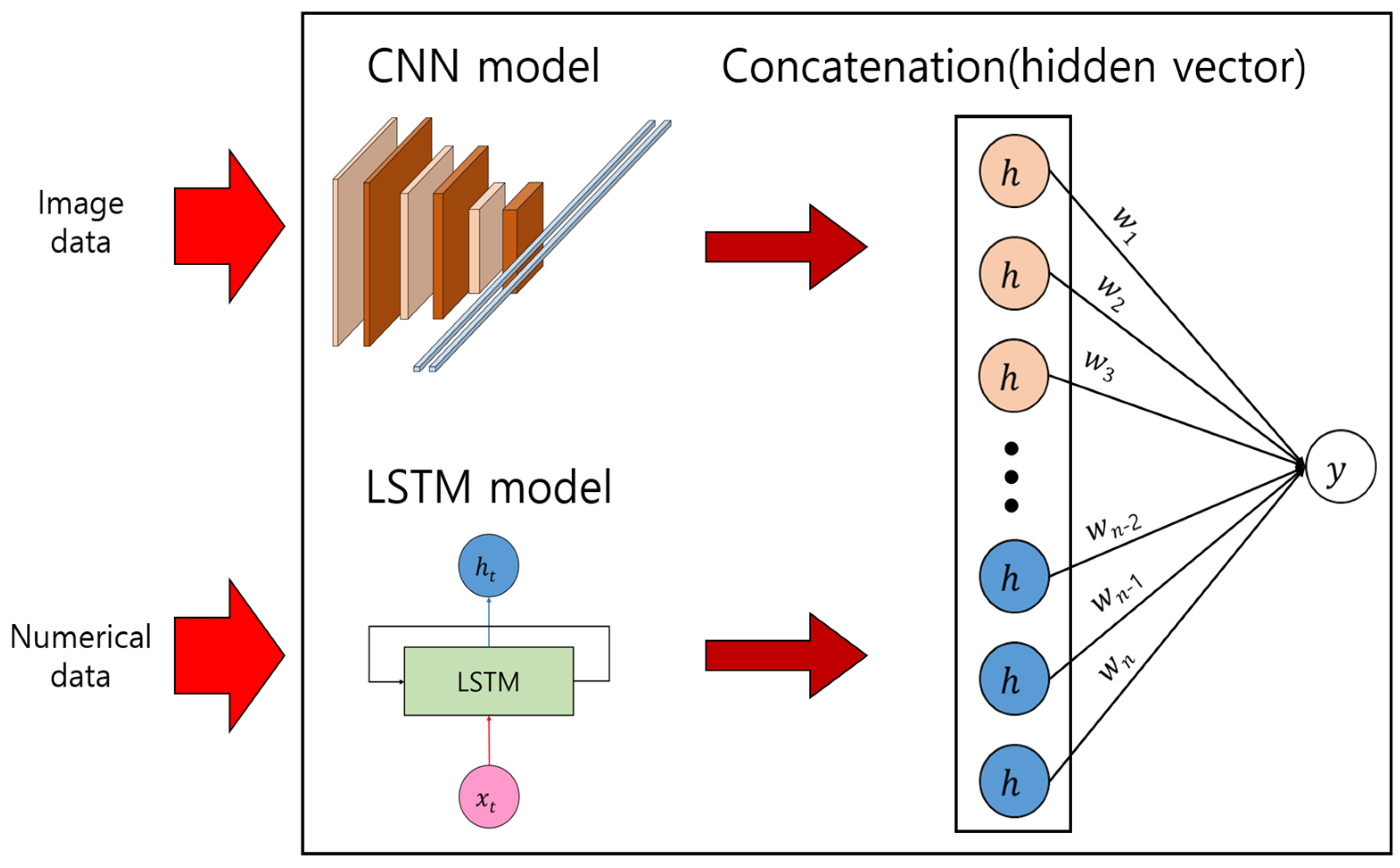
There are several data integration methods [16]. First, the integration of data dimensions is a method of embedding data of different characteristics and extracting data with the same characteristics, as shown in Figure 6. Consequently, data of different characteristics are projected into a single feature space shared. Second, integration between learned representations is a method of combining learned representations with different neural networks, as shown in Figure 7. In this paper, we use the integration of data dimension and integration between learned representations. For example, we train using CNN for image data and LSTM for time series data. Representations learned through each neural network are connected and combined with the hidden layer, and learning is performed by finding the optimal weight connected to the hidden layer.

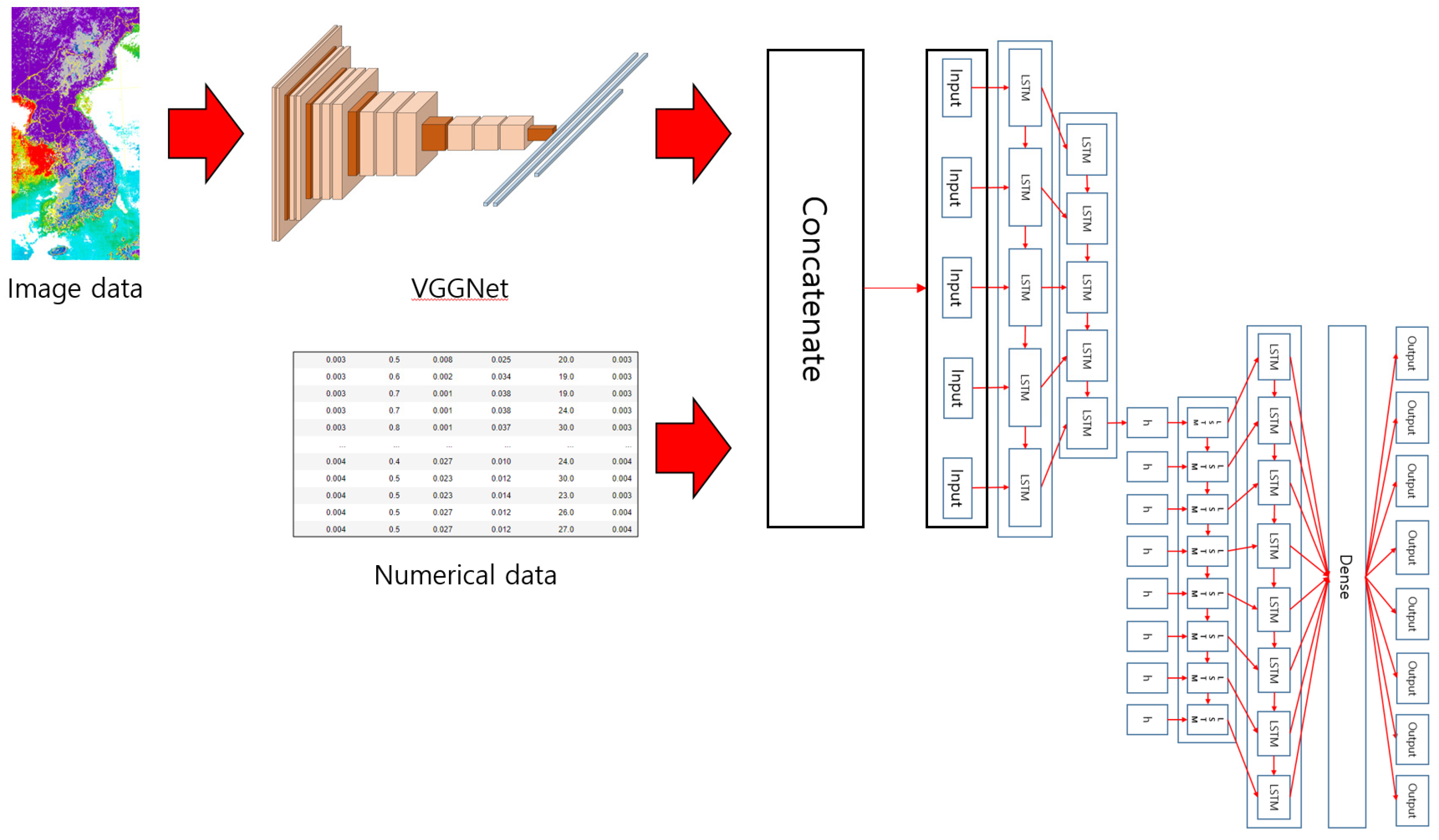
In this paper, we constructed the multimodal deep learning model, as shown in Figure 8. First, the numerical and image data are preprocessed so that data from the past 5 h can be used as input. However, the two data dimensions do not match even if the same preprocessing is performed over the preceding 5 h. Therefore, we extract the feature map for image data through a CNN-based model to preserve spatial information of the image and reshape the extracted feature map to fit the form of numerical data so that the two data can be integrated to have the same dimensional characteristics.

We used the LSTM AutoEncoder model for numerical data processing. The GRU model [17], another compact time series data handling model, is excluded because our parameters increase as numerical data and image data are merged. In this situation, the LSTM model outperforms the GRU model.

Furthermore, we used the basic CNN and VGGNet models (VGG16, VGG19) to compare performance differences according to network depth. Then, we merge the numerical data with the reshaped feature map (representations learned through the CNN-based model) via the concatenate layer. However, the data are merged so that the dimension may increase and the learning may not be good. The merged multimodal data have a time series characteristic of the past 5 h. Once the multimodal data are integrated, we feed the integrated data to the LSTM AutoEncoder in our model to reflect the dimensionality reduction and time series characteristics in the preprocessing stage.

Unlike the multimodal deep learning model of related works, our multimodal deep learning model is different because it uses a prediction model for time series data for long-term dependency learning. Kalajdjieski [8] tackles the classification problem of images as polluted or not polluted even if image and weather data are used together.

5. Optimizing Deep Learning Models

This paper optimizes the hyperparameter to maximize the performance of the model.

5.1. Hyperparameter

Hyperparameter [13] refers to a value the user must manually set when using the model. For example, learning rate, epoch, and batch size. The process of exploring optimal hyperparameters to maximize accuracy is called hyperparameter tuning, and it is never easy to find optimal values for this. If you manually substitute the value, you can find the optimal value, but it can take a very long time, and if you set the criteria incorrectly and start, you may not be able to find the optimal value. Therefore, it is necessary to find an optimal hyperparameter by selecting an appropriate search algorithm according to the implementation situation.

5.2. Katib

Katib [18] is a system that optimizes hyperparameters as a component of the Kubernetes-based machine learning platform, kubeflow. Katib uses a variety of algorithms to maximize accuracy. Typical algorithms include random search, grid search, and Bayesian optimization.

We used the random search algorithm [19] among several algorithms. Random search creates a combination of random parameters and is an excellent algorithm to use when it is impossible to explore all possibilities. We set the range of hyperparameters to experiment under various conditions. If the setting ranges of hyperparameters are all integers, the number of search cases is limited, but if the setting range includes decimal points, the number of search cases becomes very large. For example, suppose that the learning rate is expressed as a decimal point because it is between 0 and 1, and the range is set to 0.0001 and 0.001. In this case, it can be considered that the number of search cases is 100, but the number of cases is 9 × 10¹⁶ because the decimal point is measured up to 19 digits in katib. In addition, if the epoch scope is set to 0 to 100, the number of search cases is 100 × 9 × 10¹⁶. Since the number of search cases increases exponentially with the addition of several hyperparameters, such as cell size and batch size, this paper finds the optimal hyperparameter using the random search algorithm.

6. Experimental Evaluation

We evaluated the performance of newly proposed models using the dataset described in Section 3. This experiment used Python program language, Tensorflow, Keras, CentOS Linux release 9 July 2009 (Core) for software, and Intel(R) Xeon(R) Silver 4210 CPU @ 2.20 GHz, 125 GB of RAM for hardware. However, we used 90 GB of memory for model learning. LSTM AutoEncoder is denoted as LSTM_AE. In the case of the multimodal deep learning model, the model combining LSTM AutoEncoder and the basic CNN is denoted as Multimodal1, the model combining LSTM AutoEncoder and VGG16 is denoted Multimodal2, and the model combining LSTM AutoEncoder and VGG19 is denoted Multimodal3, respectively. LSTM_AE used only numerical data, and multimodal deep learning models used multimodal data. We used RMSE (Root Mean Square Error) as a performance indicator for the model’s performance evaluation. The ratio of training sets/verification sets/test sets is set to 6:2:2. The basic activation function of the LSTM layer was tanh, the cyclic activation function was sigmoid, and the activation function of the dense layer was ReLU, respectively. The optimization function was set to Adam.

Table 1. The range of hyperparameter settings for each model.

	LSTM_AE	Multimodal1 (LSTM_AE + (Basic) CNN)	Multimodal2 (LSTM_AE + VGG16)	Multimodal3 (LSTM_AE + VGG19)
Learning rate	0.00001~0.001	0.00001~0.001	0.00001~0.001	0.00001~0.001
Cell size	100~400	100~400	100~400	100~400
Batch size	20~80	20~80	20~60	20~60
Image size	120~140	120~140	120~140	120~140
Epoch	50~300	50~200	50~200	50~200

shows the range of hyperparameters considering the accuracy of each model. The contents of Table 1 are applied to katib.

For Multimodal2 and Multimodal3, which are LSTM_AE + VGGNet16/19, the maximum batch size is set to 60 because it often diverges infinitely when the batch size exceeds 60, for multimodal deep learning models (Multimodal1, Multimodal2, and Multimodal3), almost all of them diverge infinitely when the epoch exceeds 200, setting the maximum epoch to 200.

We conducted 10 experiments on each model, and

Table 2. Comparison of the performance of proposed models using the original image (Test RMSE).

Model Rank	LSTM_AE	Multimodal1	Multimodal2	Multimodal3
Rank 1	15.96	14.57	14.18	13.96
Rank 2	16.15	14.66	14.65	14.03
Rank 3	16.4	15.06	14.83	14.62
Rank 4	17.44	15.52	15.1	14.78
Rank 5	18.58	17.39	15.78	15.57
Avg of Rank	16.91	15.44	14.91	14.59

shows the top 5 in order of good performance. For the multimodal deep learning model, numerical data used the same data as LSTM_AE, and all image data used the original image data. This paper compares the performance based on the minimum and average values among the experimental results.

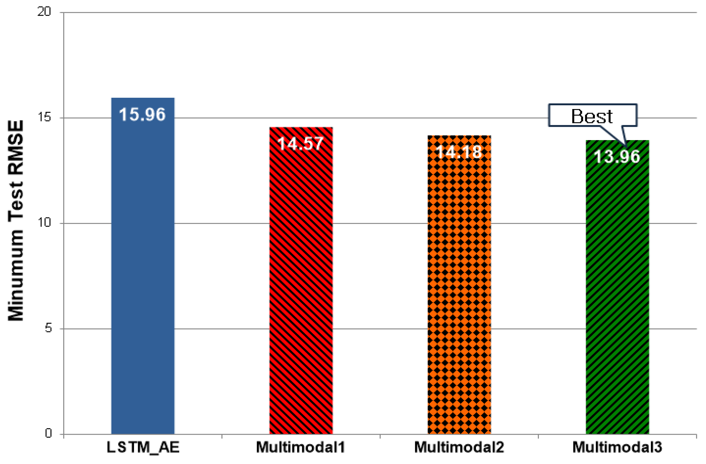
Figure 9 displays the minimum Test RMSE (Rank 1) of each model listed in Table 2. The RMSE of LSTM_AE, which processes numerical data, showed a value of 15.96, and the RMSE of Multimodal1, which is LSTM_AE + CNN, was 14.57, decreased by 8.71% compared with LSTM_AE. The RMSE of Multimodal2, LSTM_AE + VGG16, was 14.18, which decreased by 2.68% compared with Multimodal1. The RMSE of Multimodal3, LSTM_AE + VGG19, was 13.96, which decreased by 1.55% compared with Multimodal2.

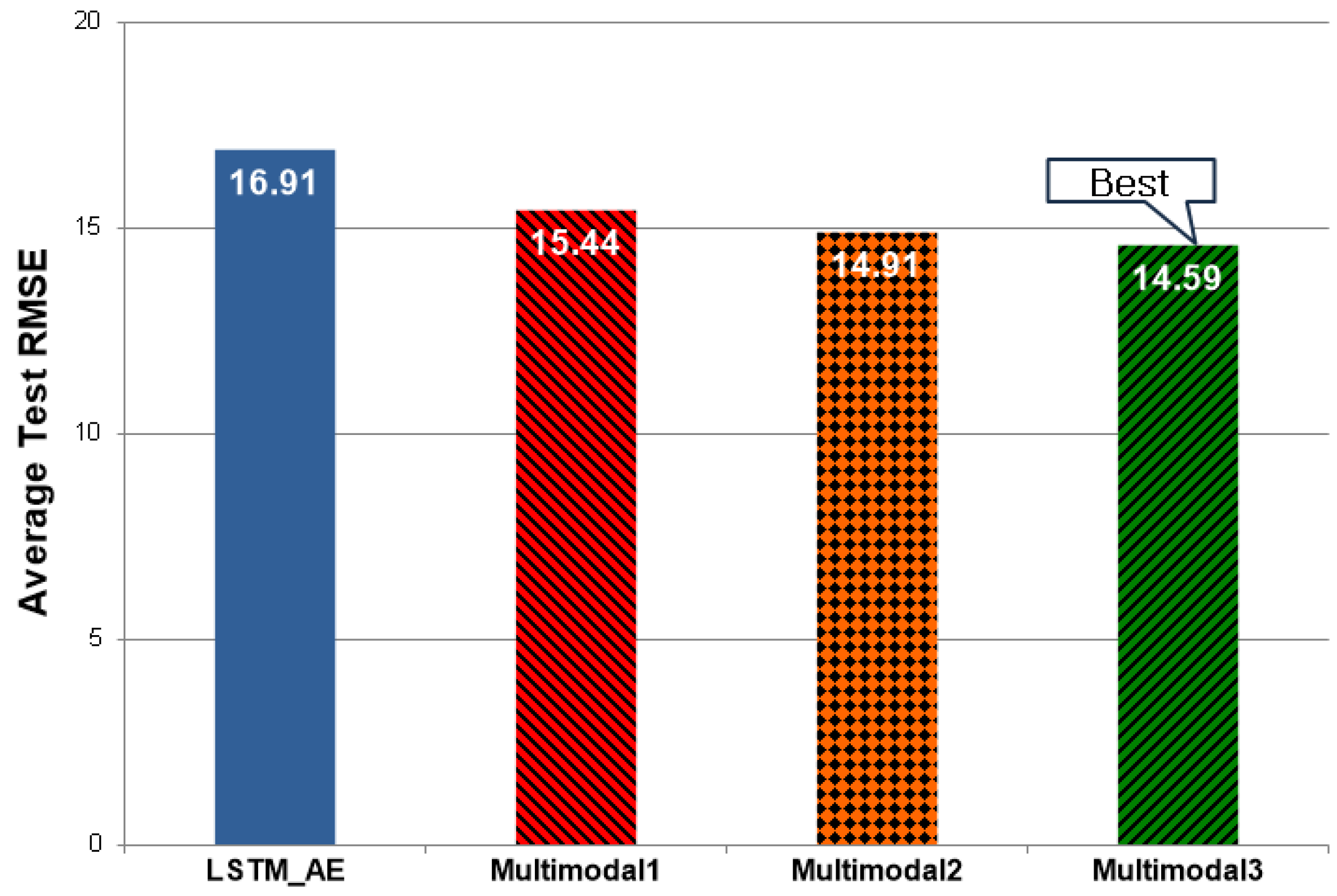
Figure 10 shows the average Test RMSE (Average of Rank) of each model shown in Table 2. The RMSE of LSTM_AE, which processes numerical data, showed a value of 16.91, and the RMSE of Multimodal1, which is LSTM_AE + CNN, was 15.44, decreased by 8.69% compared with LSTM_AE. The RMSE of Multimodal2, LSTM_AE + VGG16, was 14.91, which decreased by 3.43% compared with Multimodal1. The RMSE of Multimodal3, LSTM_AE + VGG19, was 14.59, which decreased by 2.15% compared with Multimodal2.

Table 3. Performance comparison of proposed models using cropped image (Test RMSE).

Model Rank	Multimodal1	Multimodal2	Multimodal3
Rank 1	14.03	13.88	13.7
Rank 2	14.71	15.31	14.78
Rank 3	15.28	15.51	15.12
Rank 4	16.41	15.73	15.65
Rank 5	16.71	16.27	16.14
Avg of Rank	15.43	15.34	15.01

shows the top five out of 10 experiments for proposed models in the order of good performance. However, unlike Table 2, in the case of the multimodal deep learning model, numerical data used the same data as LSTM_AE, but all image data used cropped image data. Again, the performance is compared based on the minimum and average values among the experimental results.

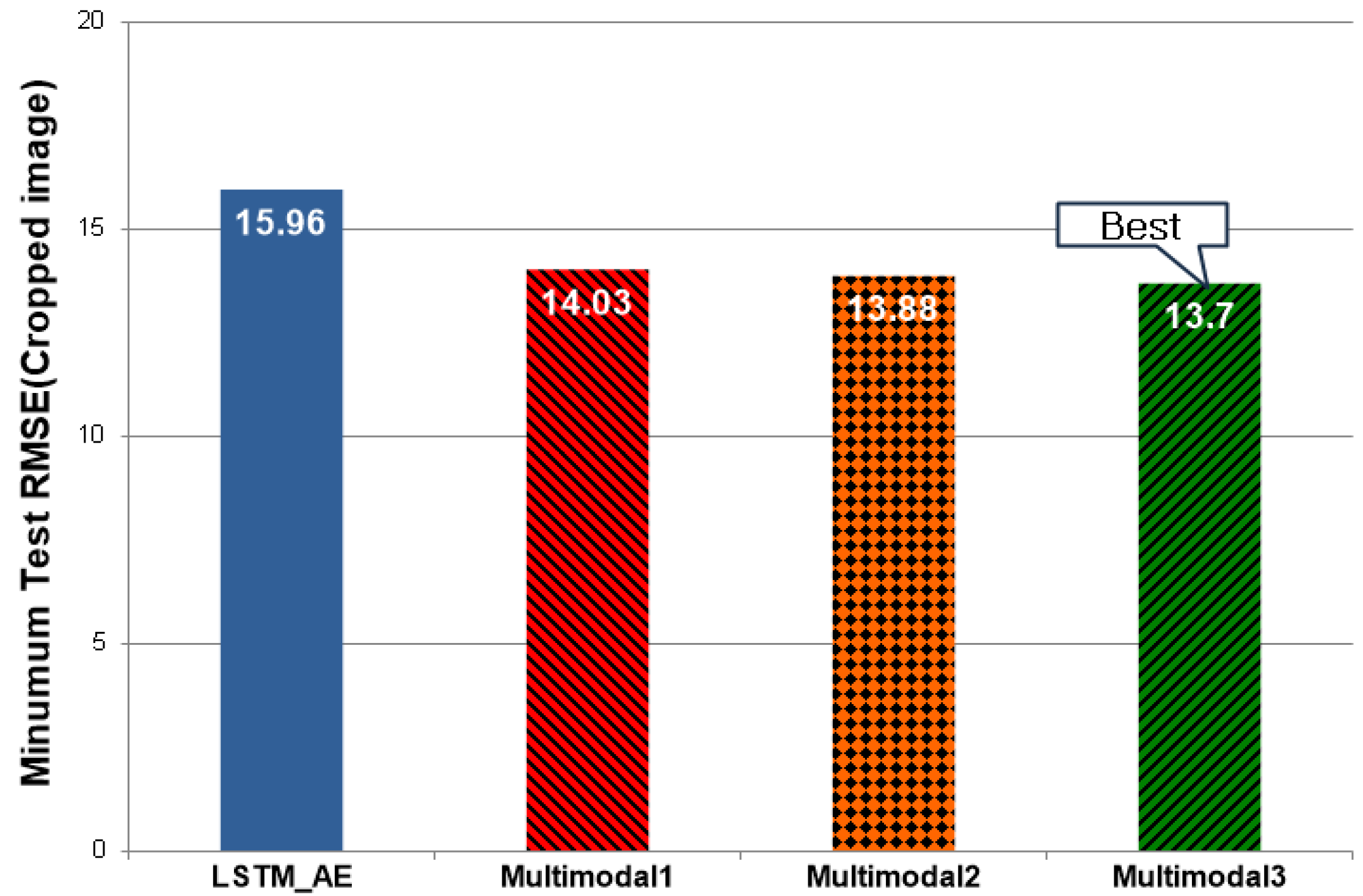
Figure 11 shows the minimum Test RMSE (Rank 1) of each model shown in Table 3. The RMSE of LSTM_AE, which processes numerical data, showed a value of 15.96, and the RMSE of Multimodal1, which is LSTM_AE + CNN, was 14.03, decreased by 12.09% compared with LSTM_AE. The RMSE of Multimodal2, LSTM_AE + VGG16, was 13.88, which decreased by 1.07% compared with Multimodal1. The RMSE of Multimodal3, LSTM_AE + VGG19, was 13.7, which decreased by 1.3% compared with Multimodal2.

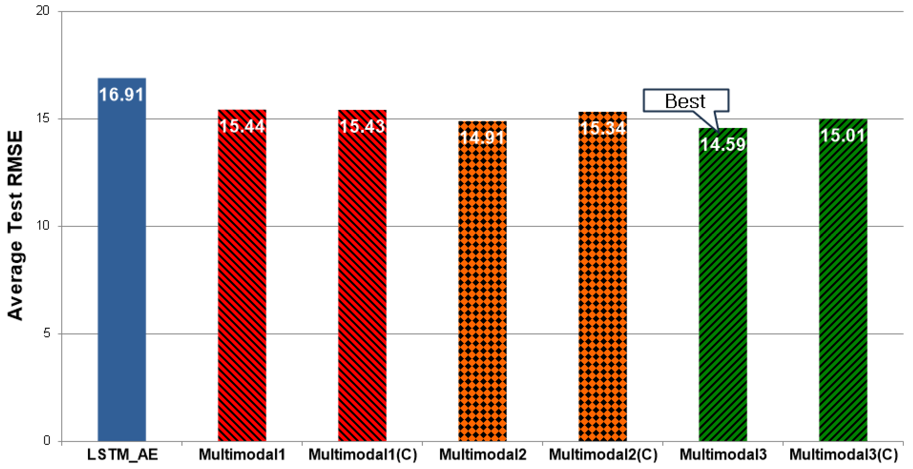
Figure 12 shows the average Test RMSE (Average of Rank) of each model shown in Table 3. The RMSE of LSTM_AE, which processes numerical data, showed a value of 16.91, and the RMSE of Multimodal1, which is LSTM_AE + CNN, was 15.43, decreased by 8.75% compared with LSTM_AE. The RMSE of Multimodal2, LSTM_AE + VGG16, was 15.34, which decreased by 0.58% compared with Multimodal1. The RMSE of Multimodal3, LSTM_AE + VGG19, was 15.01, which decreased by 2.15% compared with Multimodal2.

Figure 13 compares minimum Test RMSE for all experimental results in Table 2 and Table 3, and C means using cropped images. Overall, the performance was better when cropped images were applied, and Multimodal3(C) was the best among them.

The RMSE of Multimodal1(C) was 14.03, which decreased by 3.7% compared with Multimodal1. The RMSE of Multimodal2(C) was 13.88, which decreased by 2.11% compared with Multimodal2. The RMSE of Multimodal3(C) was 13.7, which decreased by 1.86% compared with Multimodal2.

Figure 14 compares the average Test RMSE for all experimental results in Table 2 and Table 3, and C means using cropped images. Unlike the minimum Test RMSE, the performance was not good when cropped images were applied. The RMSE of Multimodal1(C) is 15.43, which is very similar to Multimodal1, and the RMSE of Multimodal2(C) is 15.34, increased by 2.88% compared with Multimodal2. The RMSE of Multimodal3(C) was 15.01, which increased by 2.88% compared with Multimodal3.

Combining the experimental results, the multimodal deep learning model (Multimodal1, Multimodal2, Multimodal3) using both numerical and image data performed better than a single deep learning model (LSTM_AE) using only numerical data.

If the image data is the original image, the minimum Test RMSE of the multimodal deep learning model decreased by approximately 8.71–12.53% compared with the single deep learning model, and the average Test RMSE of the multimodal deep learning model was reduced by approximately 8.69–13.72% compared with the single deep learning model. If the image data is the cropped image, the minimum Test RMSE of the multimodal deep learning model was decreased by approximately 12.09–14.16% compared with the single deep learning model, and the average Test RMSE of the multimodal deep learning model was lowered by approximately 8.75–11.24% compared with the single deep learning model.

In addition, from the viewpoint of minimum Test RMSE of the multimodal deep learning model, when the cropped image was used, it decreased by approximately 1.86–3.7% compared with when the original image was used, but from the viewpoint of average Test RMSE of the multimodal deep learning model, it increased by approximately 0–2.88%.

7. Conclusions and Future Work

In this paper, we constructed the multimodal data by integrating the numerical data, the dataset in our previous study [2] showing the best performance among others, and the satellite image with aerosol information. We proposed several multimodal deep learning models by combining LSTM-based models and CNN-based models to learn the multimodal data. We also optimized the hyperparameters set of the models using katib to achieve optimal performance.

As a result, our multimodal deep learning models outperformed a single-modal deep learning model using only numerical data. In particular, Multimodal3, a model combining the deep network VGG19 among CNN-based models, performed the best. Regarding the image data, we prepared two types of image data: original images and cropped images. Regarding the minimum Test RMSE, the cropped image case performed better. However, regarding the average Test RMSE, the original image performed better.

In future work, we will explore the optimal multimodal deep learning model by applying various models in addition to those presented in the paper.

References

1. Disease Control and Prevention Agency. Available online: http://www.kdca.go.kr/contents.es?mid=a20304030300 (accessed on 19 August 2022).
2. Ko, K.K.; Shahzad, E.S.J. Big data merging and deep learning model optimization for improving weather information forecasting performance. Inst. Electron. Inf. Eng. 2021, 58, 39–46. [Google Scholar]
3. Athira, V.; Geetha, P.; Vinayakumar, R.; Soman, K. Deepairnet: Applying recurrent networks for air quality prediction. Procedia Comput. Sci. 2018, 132, 1394–1403. [Google Scholar] [CrossRef]
4. Chau, P.N.; Zalakeviciute, R.; Thomas, I.; Rybarczyk, Y. Deep Learning Approach for Assessing Air Quality During COVID-19 Lockdown in Quito. Front. Big Data 2022, 5, 842455. [Google Scholar] [CrossRef] [PubMed]
5. Salman, A.G.; Heryadi, Y.; Abdurahman, E.; Suparta, W. Single layer and multi-layer long short-term memory (lstm) model with intermediate variables for weather forecasting. Procedia Comput. Sci. 2018, 135, 89–98. [Google Scholar] [CrossRef]
6. Bekkar, A.; Hssina, B.; Douzi, S.; Douzi, K. Air-pollution prediction in smart city, deep learning approach. J. Big Data 2021, 8, 161. [Google Scholar] [CrossRef] [PubMed]
7. Xie, H.; Ji, L.; Wang, Q.; Jia, Z. Research of PM2.5 Prediction System Based on CNNs-GRU in Wuxi Urban Area. IOP Conf. Ser. Earth Environ. Sci. 2019, 300, 032073. [Google Scholar] [CrossRef] [Green Version]
8. Kalajdjieski, J.; Zdravevski, E.; Corizzo, R.; Lameski, P.; Kalajdziski, S.; Pires, I.M.; Garcia, N.M.; Trajkovik, V. Air pollution prediction with multi-modal data and deep neural networks. Remote Sens. 2020, 12, 4142. [Google Scholar] [CrossRef]
9. Ministry of Environment. Available online: http://www.me.g.,o.kr/home/web/board/read.do?pagerOffset=0&maxPageItems=10&maxIndexPages=10&searchKey=&searchValue=&menuId=286&orgCd=&boardId=1485080&boardMasterId=1&boardCategoryId=39&decorator= (accessed on 19 August 2022).
10. National Meteorological Satellite Center. Available online: http://wiki.nmsc.kma.go.kr/doku.php?id=homepage:gk2a:aep (accessed on 19 August 2022).
11. Goki, S. Deep Learning from Scratch2: Recurrent neural networks and natural language processing that are implemented and learned directly with Python; Hanbit Media: Seoul, Korea, 2017; pp. 191–287. [Google Scholar]
12. Hinton, G.E.; Salakhutdinov, R.R. Reducing the Dimensionality of Data with Neural Networks. Science 2006, 313, 504–507. [Google Scholar] [CrossRef] [PubMed] [Green Version]
13. Goki, S. Deep Learning from Scratch: Deep learning theory and implementation in Python; Hanbit Media: Seoul, Korea, 2017; pp. 107–259. [Google Scholar]
14. Karen, S.; Andrew, Z. Very deep convolutional networks for large-scale image recognition. In Proceedings of the 3rd International Conference on Learning Representations, San Diego, CA, USA, 7–9 May 2015; pp. 1–14. [Google Scholar]
15. Jiquan, N.; Aditya, K.; Mingyu, K.; Juhan, N.; Honglak, L.; Andrew, N. Multimodal deep learning. In Proceedings of the 28th international Conference on Machine Learning, Washington, DC, USA, 28 June–2 July 2011; pp. 689–696. [Google Scholar]
16. Bae, K.I.; Lee, Y.-S.; Lim, C.-W. Multi-view learning review: Understanding methods and their application. Korean J. Appl. Stat. 2019, 32, 41–68. [Google Scholar] [CrossRef]
17. Mateus, B.C.; Mendes, M.; Farinha, J.T.; Assis, R.; Cardoso, A.M. Comparing LSTM and GRU models to predict the condition of a pulp paper press. Energies 2021, 14, 6958. [Google Scholar] [CrossRef]
18. Lee, M.H.; Moon, G.-M.; Hong, S.-H.; Kim, H.-D. Kubeflow-If You Are New to Machine Learning in Kubernetes; Digital Books: Seoul, Korea, 2020; pp. 170–189. [Google Scholar]
19. James, B.; Yoshua, B. Random search for hyper-parameter optimization. JMLR 2012, 13, 281–305. [Google Scholar]
Figure 1. Satellite image with aerosol particle size information. (Source: Data from National Meteorological Satellite Center).
Applsci 12 10405 g001
Figure 2. Cropped satellite image of the Korean Peninsula.
Applsci 12 10405 g002
Figure 3. LSTM AutoEncoder model [2] with best performance when processing 5 h-old time series data entering as input, and estimated fine dust value after 1–8 h is output.
Applsci 12 10405 g003
Figure 4. Basic CNN model where number of layers does not include pooling layers. There are three convolutions and two fully connected layers, totaling five layers.
Applsci 12 10405 g004
Figure 5. VGG 16 model does not include many pooling layers, so there are 13 convolution layers and three fully connected layers, totaling 16. VGG19 has three more convolution layers than VGG16.
Applsci 12 10405 g005
Figure 6. Integration of data dimensions: embedding data of different characteristics (image and numerical data), extracting them into data with identical characteristics, and projecting them into a shared feature space.
Applsci 12 10405 g006
Figure 7. Integration between learned representations: It is a method of combining representations learned with different neural networks (CNN, LSTM). The representations learned through each neural network are connected to and combined with the hidden layer, and learning is performed in a way that finds the optimal weight connected to the hidden layer.
Applsci 12 10405 g007
Figure 8. Multimodal deep learning model: First, a feature map of image data is extracted through CNN/VGGNet. Then, the feature map and numerical data are reconstructed to have time series characteristics and merged through concatenate layer. Finally, the merged data is processed by the LSTM AutoEncoder.
Applsci 12 10405 g008
Figure 9. Minimum Test RMSE for proposed models using the original image.
Applsci 12 10405 g009
Figure 10. Average Test RMSE for each model using the original image.
Applsci 12 10405 g010
Figure 11. Minimum Test RMSE for each model using the cropped image.
Applsci 12 10405 g011
Figure 12. Average Test RMSE for each model using the cropped image.
Applsci 12 10405 g012
Figure 13. Minimum Test RMSE of all experimental results.
Applsci 12 10405 g013
Figure 14. Average Test RMSE of all experimental results.
Applsci 12 10405 g014