Early Ventricular Fibrillation Prediction Based on Topological Data Analysis of ECG Signal

Abstract

Early ventricular fibrillation (VF) prediction is critical for prevention of sudden cardiac death, and can improve patient survival. Generally, electrocardiogram (ECG) signal features are extracted to predict VF, a process which plays an important role in prediction accuracy. Therefore, this study first proposes a novel feature based on topological data analysis (TDA) to improve the accuracy of early ventricular fibrillation prediction. Firstly, the heart activity is regarded as a cardiac dynamical system, which is described by phase space reconstruction. Then the topological structure of the phase space is characterized with persistent homology, and its statistical features are further extracted and defined as TDA features. Finally, 60 subjects (30 VF, 30 healthy) from three public ECG databases are used to validate the prediction performance of the proposed method. Compared to heart rate variability features and box-counting features, TDA features achieve a superior accuracy of 91.7%. Additionally, the three types of features are combined as fusion features, achieving the optimal accuracy of 95.0%. The fusion features are then ranked, and the first seven components are all from the TDA features. It follows that the proposed features provide a significant effect in improving the predictive performance of early VF.

1. Introduction

Ventricular tachyarrhythmia (VTA) is the main cause of sudden cardiac death (SCD) [1] and includes different types of arrhythmias such as ventricular tachycardia (VT) or ventricular fibrillation (VF), which account for approximately 80% of SCD [2]. When VF occurs, this arrhythmia can lead to cardiac arrest, leaving the patient unconscious and with no pulse at all. Due to the short duration between onset and death, it is difficult for patients to be resuscitated in time. Therefore, early prediction and warning of VF is a very critical issue to raise the survival rate of patients.

Currently, VF prediction methods are mostly performed using electrocardiogram (ECG) signals, mainly based on deep learning (DL) and machine learning (ML). For DL, Tseng et al. used a convolutional neural network (CNN) model to predict VF 5 min in advance and obtained an accuracy of 88%, using a total of 65 ECG records for training [3]. The prediction accuracy of DL methods is often lower than that of ML methods, due to the limitation of data volume. Therefore, ML is widely applied to predict VF.

For ML methods, the forecast time of VF first needs to be determined, including long lengths of 10 min or more, medium lengths of 4–6 min, and short lengths focused on 0–1 min. In terms of long length, few databases are available for long-time monitoring. For example, Mandala et al. predicted VF 15 min in advance with 18 ECG records [4], and Ebrahimzadeh et al. predicted VF 13 min in advance with 41 ECG records [5]. In terms of short length, Taye et al. used 55 ECG records to predict VF 30 s in advance [6], and Joo et al. used 78 ECG records to predict VF 10 s in advance [7]. The databases are more adequate when the prediction is very close to the VF onset, leaving insufficient warning time for resuscitation. In terms of medium lengths, Khazaei et al. predicted VF 5 min in advance with an accuracy of 95% using 38 ECG records [8], and Heng et al. predicted VF 4 min 31 s in advance with an accuracy of 98.44% using 64 ECG records [9]. There are adequate databases available for medium length predictions with sufficient warning time, so this study focuses on the forecast time of medium lengths for VF prediction.

Moreover, feature extraction plays an essential role in VF prediction accuracy. Heart rate variability (HRV) estimation has been used as the main feature to predict VF [10,11], including time domain [5,7], frequency domain [7], time-frequency [5,12], and nonlinear domain [5,8,12]. In addition, morphological features of ECG signals have also been employed to predict VF [13], such as QRS interval and Q-wave peak [4], as well as T-wave, ST-segment, and QT interval [14]. Recently, phase space reconstruction (PSR) has been applied to observe the nonlinear dynamical behavior of ECG series for VF prediction. PSR treats heart activity as a nonlinear dynamical system, which can be mapped from a one-dimensional time series to a multidimensional space using time-delay embedding parameters [15,16]. The box-counting method is commonly used for extracting statistical features from PSR trajectories [17]. For ECG-based VF prediction, statistical features mainly include mean (μ), variance (σ), skewness (γ), coefficient of variation (CV), kurtosis (β), J index, and self-similarity features [9,18,19,20]. It follows that the PSR method is feasible to predict VF. Topological data analysis (TDA) features characterize the internal topological structure of PSR trajectories and are sensitive to the weak changes of ECG signals. Therefore, we propose a TDA-based VF prediction method to improve prediction accuracy.

The main contributions of this study are listed as follows: (1) TDA features of ECG are first proposed to predict VF in this study, contributing a new insight for characterizing nonlinear dynamical behavior of ECG signal. (2) The influence of PSR reconstruction parameters combined with split frame lengths on the accuracy of VF prediction is investigated for the first time, providing an opportunity to mitigate the limitations caused by empirical parameters. (3) Compared to previous ECG-based VF prediction methods, the forecast time of the proposed method is effectively advanced with sufficient data volume and comparable prediction accuracy. Therefore, this study provides an effective features extraction method for early VF prediction.

The remainder of the study is structured as follows: Section 2 outlines the materials and methods, followed by Section 3 which presents the experimental results of the methods used in this study, while Section 4 contains a discussion of the results, a comparison of the results to other methods, and conclusions.

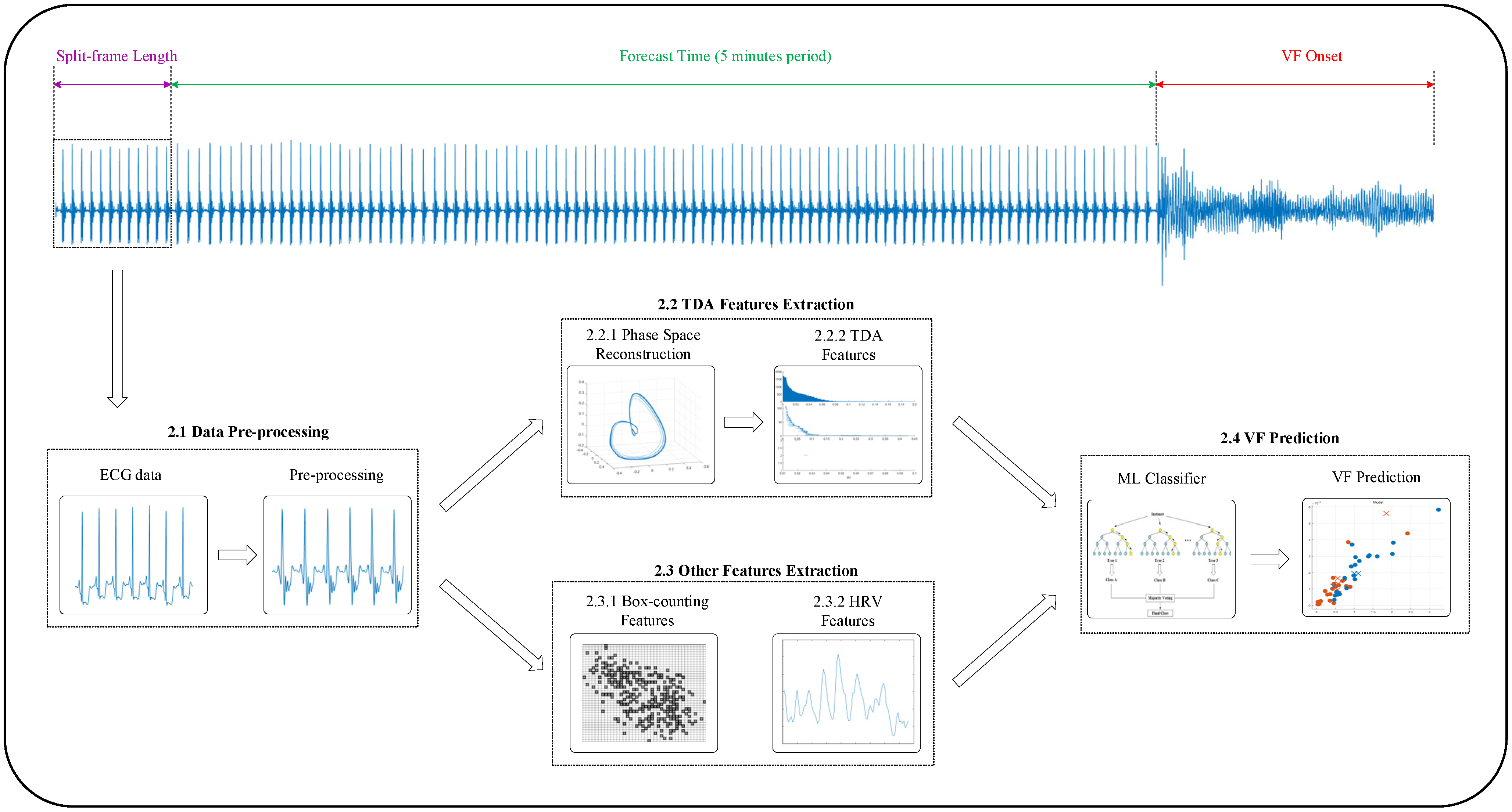
2. Materials and Methods

A flow chart of the VF prediction proposed in this study is shown in Figure 1.

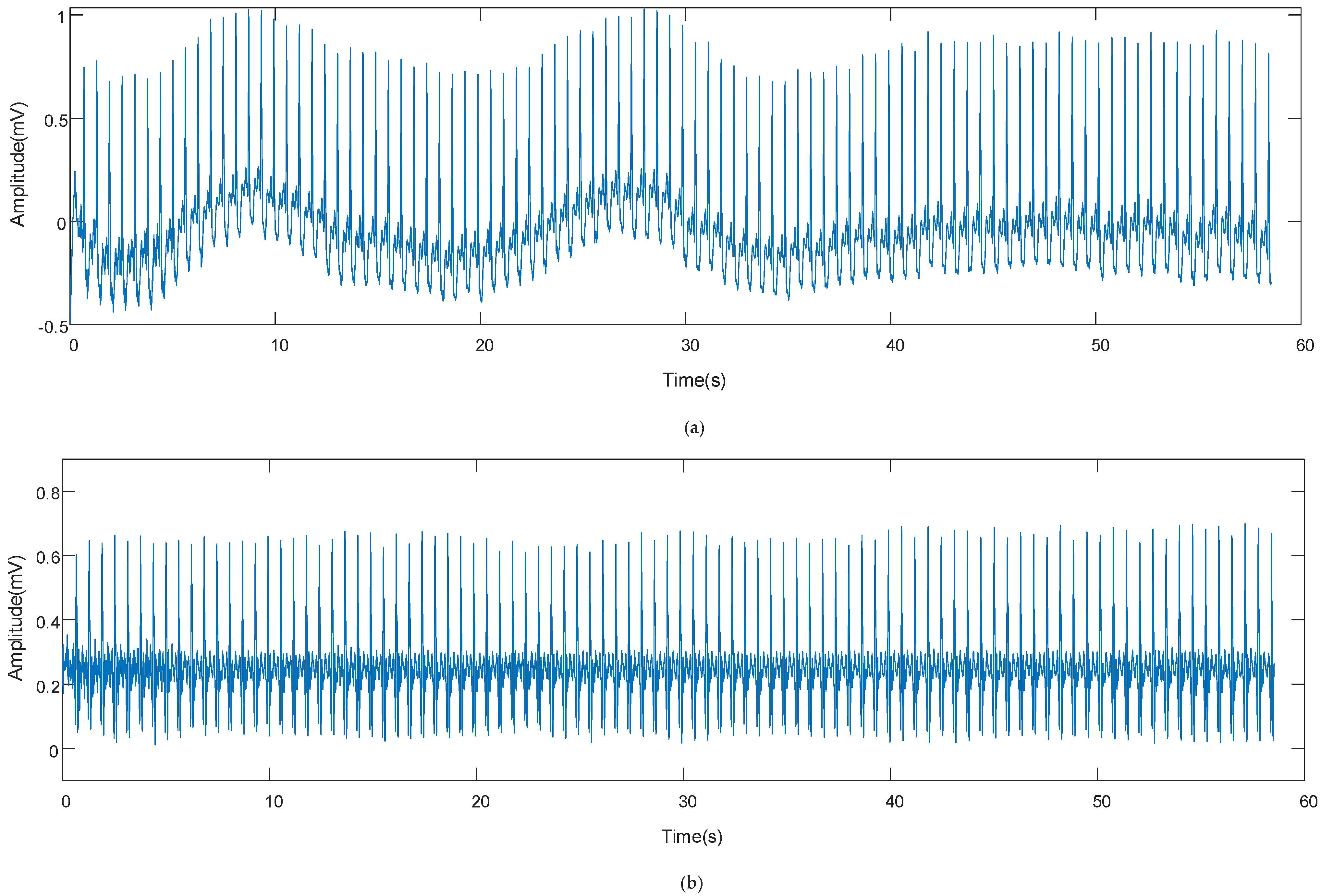
2.1. Data Pre-Processing

Three public databases from PhysioNet are utilized in this study, including Creighton University Ventricular Tachyarrhythmia Database (CUDB), Sudden Cardiac Death Holter Database (SDDB), and Physikalisch-Technische Bundesanstalt Diagnostic ECG Database (PTBDB). CUDB consists of 35 eight-minute ECG records at a sampling rate of 250 Hz, from individuals presenting sustained ventricular tachycardia, ventricular flutter, and VF [21]. The records in SDDB were obtained primarily at Boston-area hospitals in the 1980s, and currently include 18 subjects with basal sinus rhythm (four with intermittent pacing, one with persistent rhythm, and four with atrial fibrillation), with records digitized at 250 Hz. All subjects sustained ventricular tachyarrhythmias and most suffered actual cardiac arrest [22]. The ECG records collected in PTBDB are obtained using a non-commercial PTB prototype logger and contain 549 records from 290 subjects at a sampling rate of 1000 Hz, 52 of whom are healthy controls [23]. In CUDB, some patients have less than 5 min of recording time before the onset of VF and were eliminated to meet the requirement of forecast time. In SDDB, four data labeled as atrial fibrillation, two data without VF onset time, and two VF data with poor signal-to-noise ratio were removed. Thirty subjects were selected from CUDB and SDDB as VF data. To balance the two types of data, 30 healthy subjects were selected from PTBDB as non-VF (nVF) data. All 60 selected records are shown in

Table 1. Sixty selected ECG records from CUDB, SDDB, and PTBDB.

Database	Data	Sampling Rate
CUDB	‘cu10′; ‘cu11′;‘cu13′;‘cu24′;‘cu17′;‘cu22′;‘cu23′; ‘cu05′;‘cu15′;‘cu19′;‘cu32′;‘cu33′;‘cu03′;‘cu14′;‘cu18	250 Hz
SDDB	31;32;33;34;35;36;37;38;44;45;46;47;48;50;51	250 Hz
PTBDB	‘s0552_re’;‘s0551_re’;‘s0543_re’;‘s0534_re’;‘s0533_re’;‘s0532_re’;‘s0531_re’;‘s0527_re’;‘s0526_re’;‘s0506_re’;‘s0504_re’;‘s0503_re’;’s0502_re’;’s0500_re’;’s0499_re’;’s0496_re’;’s0491_re’;‘s0487_re’;‘s0486_re’;‘s0481_re’;‘s0480_re’;‘s0479_re’;‘s0478_re’;‘s0474_re’;‘s0473_re’;‘s0472_re’;‘s0471_re’;‘s0470_re’;‘s0469_re’;‘s0468_re’	1000 Hz

.

For pre-processing, the nVF data from PTBDB were first downsampled to 250 Hz. Then, both VF and nVF data were passed through a moving average filter with a window length of 10 samples to remove the baseline drift caused by the subject’s breathing; a 50 Hz band stop filter was applied to eliminate industrial frequency interference. Finally, normalization was applied to draw the distinction among the three databases by unifying the signal amplitudes to a range between 0 and 1. Figure 2 shows the results of the pre-processing.

After pre-processing, the ECG split frame was intercepted from each VF data, as shown in Figure 1. In this study, the forecast time was selected as 5 min, and the split frame lengths were selected as 5 s, 8 s, 10 s, and 15 s, respectively. For the control data, the same length of the split frame was intercepted from each nVF data.

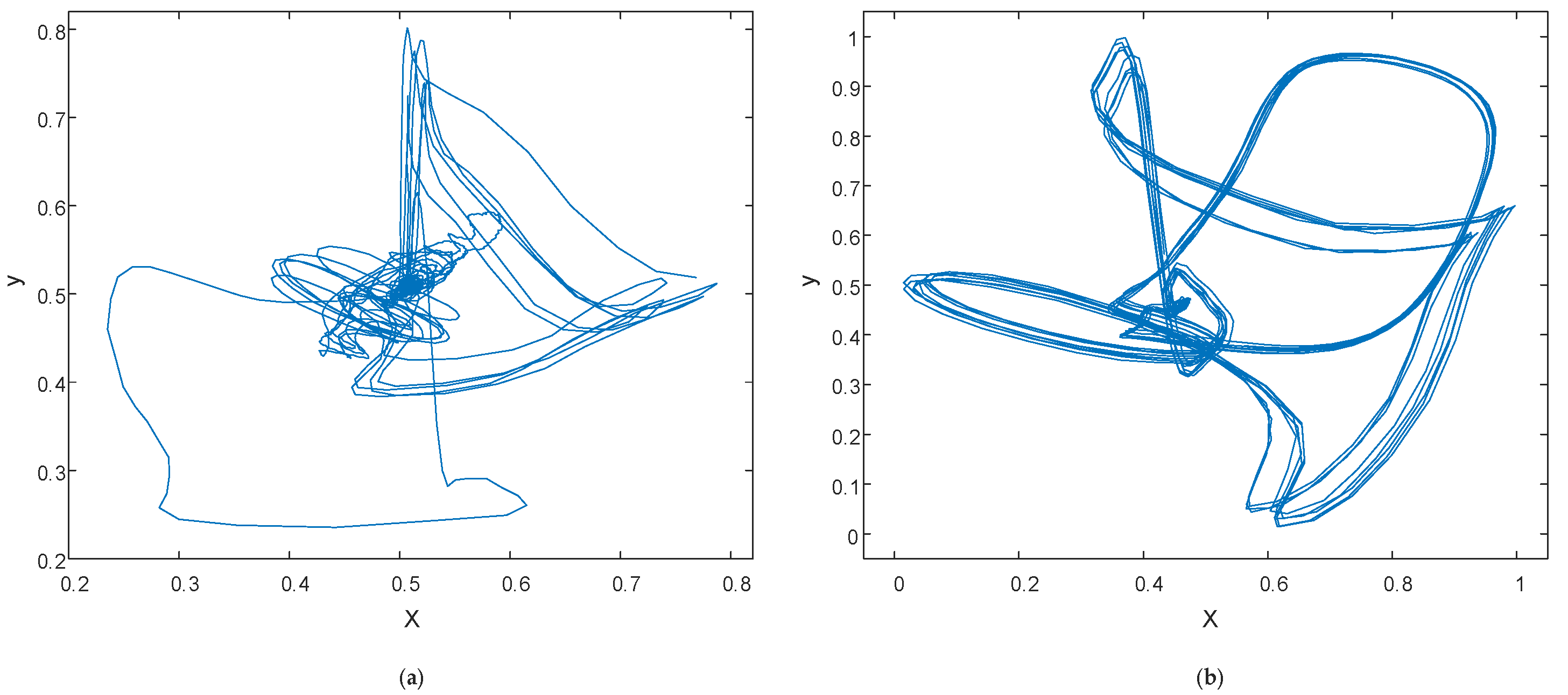
2.2. TDA Features Extraction

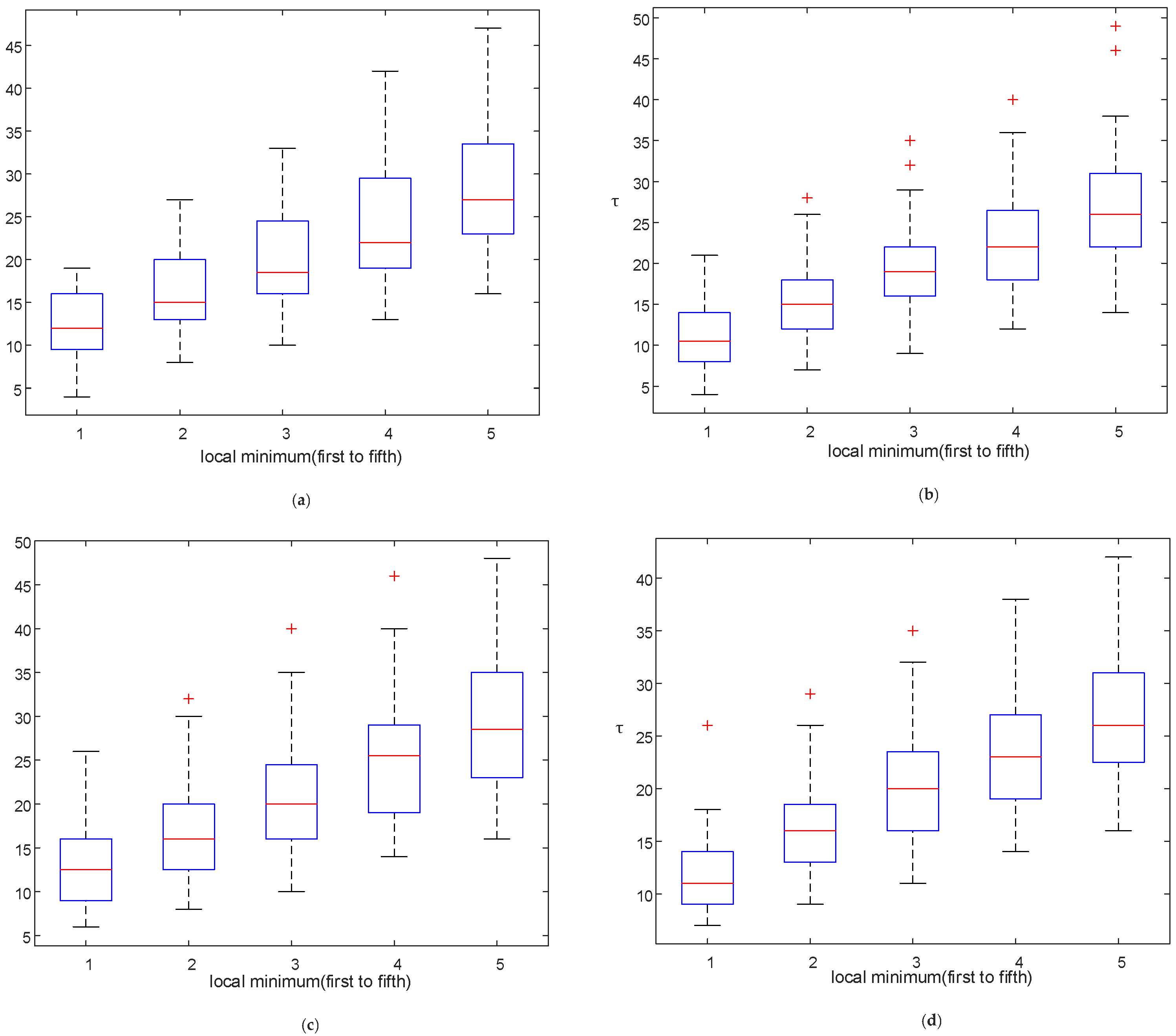
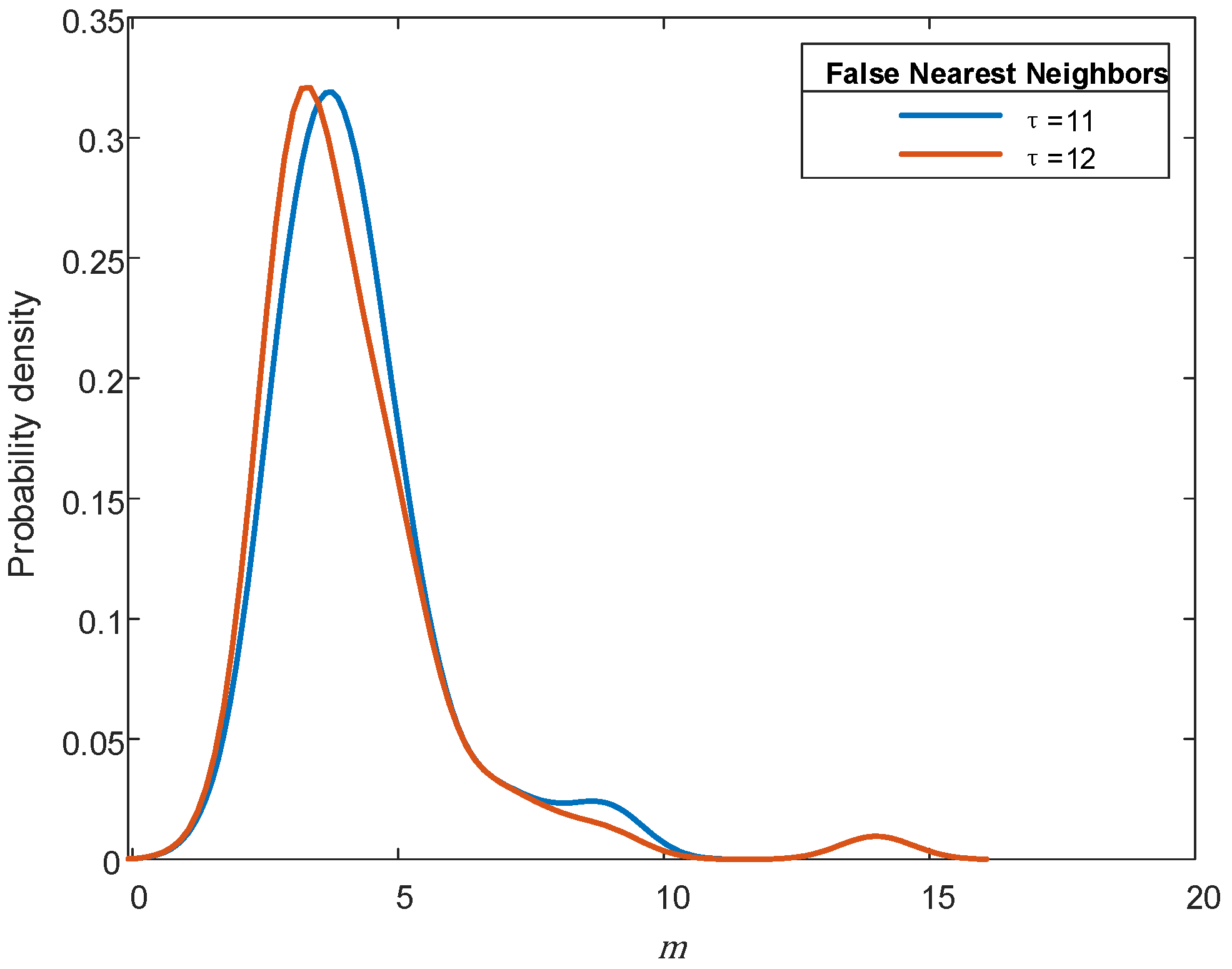
2.2.1. Phase Space Reconstruction

Takens’ study, presented in the 1980s, is an important theoretical basis for PSR [24], revealing the dynamical mechanism of nonlinear systems. As stated in Takens’ theorem, a phase space can be reconstructed from a one-dimensional chaotic time series, which is equivalent to the original system in a topological structure. Therefore, PSR is able to capture the effective information about the system from a univariate time series.

Takens’ theorem $M$ is a $d$-dimensional manifold, the map $\phi :M\to M$ is a smooth differential homogeneous embryo, and the map $y:M\to R$ has continuous second-order derivatives $\Phi \left(\phi ,y\right):M\to R^{2d+1}$, which are described as Formula (1).

$$\Phi \left(\phi ,y\right)=\left(y\left(x\right),y\left(\phi \left(x\right)\right),y\left({\phi }^2\left(x\right)\right),\dots ,y\left({\phi }^{2d}\left(x\right)\right)\right),$$

(1)

Then, $\Phi \left(\phi ,y\right)$ results in the embedding of $M$ into $R^{2d+1}$.

The current PSR commonly uses the coordinate delay reconstruction method proposed by Packard et al. [25], which essentially uses a fixed time delay $0,\tau ,2\tau ,\dots ,\left(m-1\right)\tau$ in a one-dimensional time series $\left\{x\left(t\right)\right\}$ to construct the $m$-dimensional phase space vector:

$$X\left(t\right)=\left\{x\left(t\right),x\left(t+\tau \right),x\left(t+2\tau \right),\dots x\left(t+\left(m-1\right)\tau \right)\right\}.$$

(2)

The phase space trajectory of the signal can be plotted as follows: plot $x\left(t\right)$ on the x-axis and $x\left(t+\tau \right)$ on the y-axis. Such a trajectory is called a two-dimensional phase space image. To generate a higher dimensional phase space trajectory, the embedding dimension $m$ requires to be raised and more delay sequences need to be inserted [17].

Therefore, two important reconstruction parameters need to be determined: time delay $\tau$ and embedding dimension $m$. $\tau$ and $m$ can take arbitrary values for ideal one-dimensional time series, which are infinitely long and noiseless. However, the time series in practice are finite and noisy, so $\tau$ and $m$ cannot be taken arbitrarily, which may affect the effect of PSR.

The criterion for choosing $\tau$ is to make the original sequence and the delayed sequence linearly independent from each other, so that they can be treated as independent coordinates in the reconstructed phase space. Primary choosing methods include auto-correlation function (ACF) [26], average mutual information (AMI) [27], and average displacement (AD) [28]. In this study, the AMI method is applied to determine $\tau$. The mutual information (MI) describes the correlation between two variables, which can be calculated by correlation entropy. When the MI function reaches the minimum, the corresponding $\tau$ is the appropriate time delay.

For the embedding dimension $m$, it can be derived from Takens’ theorem that the ideal reconstruction can be achieved when $m$ is large enough, but the computational effort increases exponentially with the increase of $m$. Therefore, it is necessary to find the minimum embedding dimension $m$ that is sufficient for embedding. The common methods are singular value decomposition (SVD) [29] and false nearest neighbors (FNN) [30]. In this study, the FNN method is applied to determine $m$. When two points that are not adjacent in the $d$-dimensional space become adjacent in the ($d$-1)-dimensional space, they are called false neighbors. As $m$ increases, the embedding becomes progressively sufficient, and the false neighbors are eliminated. When the false neighbors no longer decrease with the increase of $m$, the trajectory is considered to be sufficiently embedded, and the optimal $m$ is obtained. Assuming that two points in one-dimensional time series are neighbors, the distance between them is calculated. With the increase of $m$, if the embedding changes the distance between the neighbors appreciably, they are regarded as false neighbors.

Figure 3 illustrates the phase space trajectories of a 10 s VF split frame and a 10 s nVF split frame when $m$ is chosen as 2 and $\tau$ is chosen as 12.

As shown in Figure 3, PSR reconstructs attractors through finite data to observe the behavior of the dynamic system. For the nVF split frame in Figure 3b, the curves in the phase space image show a regular structure with a compact distribution of trajectories. For the VF split frame in Figure 3a, the curves fill the region in an irregular manner, which is caused by the abnormal heart rhythm, resulting in an obvious difference between the phase space trajectories of VF and nVF. PSR effectively distinguishes between VF and nVF split frames, whose structures can be statistically characterized by TDA.

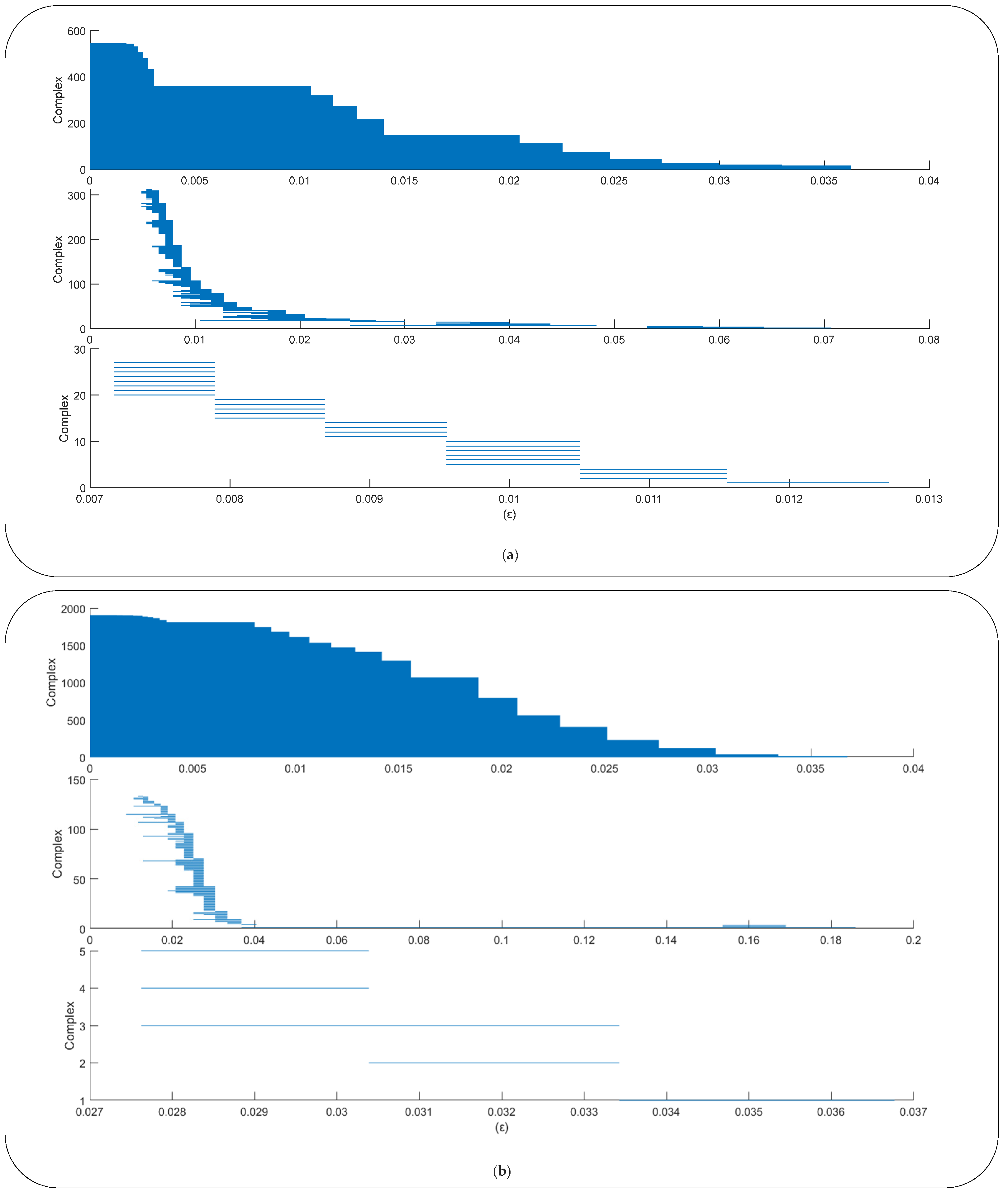
2.2.2. Topological Data Analysis

TDA provides insight into the underlying structure in data points of various dimensions [31], making it effective for the analysis of high-dimensional phase trajectory obtained by PSR, which is also considered as a high-dimensional point cloud due to its discrete form. Persistent homology (PH) is a TDA method for describing the latent structure of a point cloud which is computed during the filtration of the point cloud. Point cloud filtration using the Rips complex has been used for ECG analysis and has been proved to be effective, for example for atrial fibrillation detection [32]. Therefore, this study employs Rips complex filtration for TDA feature extraction.

PH can be characterized by the Betti number, which implies $n$-dimensional holes in the Rips complex. Since the period between the start of the hole and its disappearance is considered as PH, it can be presented as a barcode, which is a table of PH and its corresponding Betti numbers [32]. Figure 4 demonstrates the barcode diagrams of a 10 s VF split frame and a 10 s nVF split frame when $m$ is chosen as 6 and $\tau$ is chosen as 12.

In this study, the SimBa method is used to obtain approximate results of Rips filtration for improving computational efficiency [33], and the extraction procedure of TDA features is described as follows:

• Obtain the barcode from the point cloud;
• Calculate the PH duration length (PHDL) of each complex during the filtration process, which is defined as the difference between the radius when the complex disappears and the radius when the complex appears:

  $${\mathrm{PHDL}}_b\left(i\right)={\epsilon }_{\mathrm{disappear}}-{\epsilon }_{\mathrm{appear}}\left(i=1, 2, 3, 4, \dots , \mathrm{N}\right),$$

  (3)

  where b is the Betti number, $\epsilon$ is the radius during the filtration process, and there are $\mathrm{N}$ complexes in the barcodes; and,
• Finally, the three statistical features of PHDL in the barcodes with Betti number b are calculated as follows:

$${\mathrm{sum}}_b={\displaystyle \sum }_{i=1}^{\mathrm{N}}{\mathrm{PHDL}}_b\left(i\right),$$

(4)

$${\mathrm{mean}}_b=\frac{1}{\mathrm{N}}{\displaystyle \sum }_{i=1}^{\mathrm{N}}{\mathrm{PHDL}}_b\left(i\right),$$

(5)

$${\mathrm{var}}_b=\frac{1}{\mathrm{N}-1}{\displaystyle \sum }_{i=1}^{\mathrm{N}}{\left|{\mathrm{PHDL}}_b\left(i\right)-{\mathrm{mean}}_b\right|}^2$$

(6)

Totally, nine TDA features were calculated from the point clouds obtained from PSR; they are listed in

Table 2. Defined nine TDA features.

Features	TDA 0	TDA 1	TDA 2
Sum	sum 0	sum 1	sum 2
Variance	var 0	var 1	var 2
Mean	mean 0	mean 1	mean 2

.

2.3. Other Features Extraction

To evaluate the performance of the proposed TDA features, we extracted box-counting features and HRV features using the same ECG data.

2.3.1. Box-Counting Features

In the box-counting method, the embedding dimension $m$ is usually assigned a value of 2, allowing the inscription of a two-dimensional phase-space image describing the trajectory of the system [17,34]. Box-counting method can characterize the signal complexity and identify potential ECG signal desynchronization phenomena [20]. After obtaining the phase space image, it is exported as a 1024 × 1024 high-resolution grayscale image. The pixels in the image are counted as “black box” if the pixel value is 0 and as “white box” if the pixel value is 1. The black-box pixels represent the measure of trajectory spreading, so it will be counted to calculate statistical parameters named as box number $n_b$. In this study, two parameters, $CV$ and $\kappa$, were calculated with sliding windows. $CV$ is the distribution of the trajectory normalized by the mean, which is the ratio of the standard deviation ($\sigma$) to the mean ($\mu$).

$$\mu =\frac{1}{\mathrm{N}}{\displaystyle \sum _{i=1}^{\mathrm{N}}}{n}_b\left(i\right),\sigma =\sqrt{\frac{1}{\mathrm{N}}{\displaystyle \sum _{i=1}^{\mathrm{N}}}{\left(n_b\left(i\right)-\mu \right)}^2,}\left(i=1, 2, 3, 4, \dots , \mathrm{N}\right)$$

(7)

$$CV=\frac{\sigma }{\mu },$$

(8)

$\kappa$ is the fourth-order statistical moment of the box number, measuring whether the data distribution is steeper or flatter relative to the normal distribution [18].

$$\kappa =\sqrt{\frac{1}{\mathrm{N}}{\displaystyle \sum _{i=1}^{\mathrm{N}}}{\left[\left(n_b\left(i\right)-\mu \right)/\sigma \right]}^4,}\left(i=1, 2, 3, 4, \dots , \mathrm{N}\right),$$

(9)

where $\mathrm{N}$ is the number of sliding windows.

2.3.2. HRV Features

For ECG signal, the R-peak is detected to obtain the R-R interval (RRI) sequence. In this study, 7 HRV features were calculated using mean value ($MNN$), standard deviation ($SDNN$), root mean square of continuous difference ($RMSSD$), $NN50$, $PNN50$, $skewness,$ and $kurtosis$ of RRI sequence: all are shown in

Table 3. Seven HRV features.

Features	Equation
$MNN$	${\displaystyle \sum _{i=1}^{\mathrm{N}}}\mathrm{Y}\left(i\right)/\mathrm{N}$
$SDNN$	$\sqrt{{\displaystyle \sum _{i=1}^{\mathrm{N}}}{\left(\mathrm{Y}\left(i\right)-MNN\right)}^2/\mathrm{N}}$
$RMSSD$	$\sqrt{{\displaystyle \sum _{i=1}^{\mathrm{N}}}{\left(\mathrm{Y}\left(i+1\right)-\mathrm{Y}\left(i\right)\right)}^2/\left(\mathrm{N}-1\right)}$
$NN50$	The number of RRI sequences where the difference between adjacent terms is greater than 50 ms
$PNN50$	The ratio of the number of adjacent terms in RRI sequence whose difference is greater than 50 ms to the sequence length
$skewness$	${\mathrm{M}}_3\sqrt{{({\mathrm{M}}_2)}^3}$
$kurtosis$	$\frac{{\mathrm{M}}_4}{{({\mathrm{M}}_2)}^2}-3$

Where $\mathrm{Y}$ is an RRI sequence, $\mathrm{N}$ is the number of data points in the RRI sequence, ${\mathrm{M}}_k$ is the $k$ statistical moment of RRI sequence.

[10,11].

2.4. VF Prediction

To distinguish VF from nVF, nine TDA features, two box-count features, and seven HRV features were fed into 5 ML classifiers, respectively, including decision tree (DT), random forest (RF), logistic regression (LR), support vector machine (SVM), and k-nearest neighbor (KNN). VF was predicted when the output was 1, while nVF was predicted when the output was 0. Accuracy was used as the performance indicator:

$$\mathrm{Accuracy}=\frac{\mathrm{TP}+\mathrm{TN}}{\mathrm{TP}+\mathrm{TN}+\mathrm{FP}+\mathrm{FN}}$$

(10)

where TP is true positive, TN is true negative, FP is false positive, and FN is false negative.

3. Results

3.1. Reconstruction Parameter Determination

For the determination of $\tau$, the AMI method was used in this study. Based on the split frame lengths of 5 s, 8 s, 10 s, 15 s, MI functions of 60 split frames were calculated individually; when the MI function of each split frame reached the first to the fifth local minima, the corresponding $\tau$ values were recorded. Figure 5 illustrates the distribution of $\tau$ values of each local minimum for the four split frame lengths with box plot, including its upper and lower edges, median, and outliers.

As shown in Figure 5, the box plots demonstrate a widening trend from the first to the fifth local minimum, indicating that MI is becoming dispersed. To achieve the minimum value of MI, the median of the first local minimum was selected as the appropriate value of $\tau$. For the split frame lengths of 5 s, 8 s, 10 s, 15 s, the range of $\tau$ was 10.5–12.5, so the integer 11 or 12 was chosen as the optimal value of $\tau$.

For the calculation of $m$, the FNN method was used in this study. After selecting $\tau$ as 11 and 12, their respective probability density curves of $m$ were plotted (Figure 6). The two curves are tangent at $m$ = 6, and 83% of the data are sufficient for embedding. Considering the limitation of the computational effort, six was taken as the value of $m$.

3.2. Split Frame Length Selection

From Figure 5, it can be observed that there is an interaction between the split frame length and the reconstruction parameter $\tau$ which probably influences the performance of classifier. Therefore, four split frame lengths (5 s, 8 s, 10 s, and 15 s) and two $\tau$ values (11 and 12) were paired to extract TDA features. Five ML classifiers were used to predict VF, and the superior classifiers are listed in

Table 4. VF prediction accuracy of superior classifiers.

$\mathit{\tau }$	5 s Split Frame	8 s Split Frame	10 s Split Frame	15 s Split Frame
11	90.0% RF	86.7% RF	88.3% DT	83.3% DT
12	91.7% RF	93.3% RF	88.3% RF	83.3% RF

with their accuracy.

As shown in Table 4, DT and RF demonstrate superior classification performance. For the value of $\tau$, the accuracy of 12 is generally higher than that of 11, so optimal $\tau$ was selected as 12. Moreover, with increasing split frame length, the accuracy gradually decreases; as a result, optimal split frame length was chosen as 5 s.

3.3. Prediction Performance Comparison

To evaluate the performance of the proposed TDA features, we extracted the box-counting features and HRV features with 60 ECG split frames. In addition, nine TDA features, two box-counting features, and seven HRV features were combined to form 18 fusion features vector. Then, all types of the features were respectively fed into 5 ML classifiers. The classification accuracy with 10-fold cross-validation is shown in

Table 5. Combination of different types of features and classifiers.

ML Classifiers	Box-Counting Features	HRV Features	TDA Features	Fusion Features
Decision Trees	70.0%	61.7%	86.7%	91.7%
Logistic Regression	65.0%	56.7%	53.3%	55.0%
SVM	71.7%	71.7%	55.0%	55.0%
KNN	63.3%	66.7%	55.0%	53.3%
Radom Forest	61.7%	65.0%	91.7%	95.0%

Where $m$ is 6, $\tau$ is 12, and split frame length is 5 s.

.

It can be seen that the accuracy obtained by TDA features is significantly higher than that of the other two types of features, respectively; prediction performance was further improved by fusing the features.

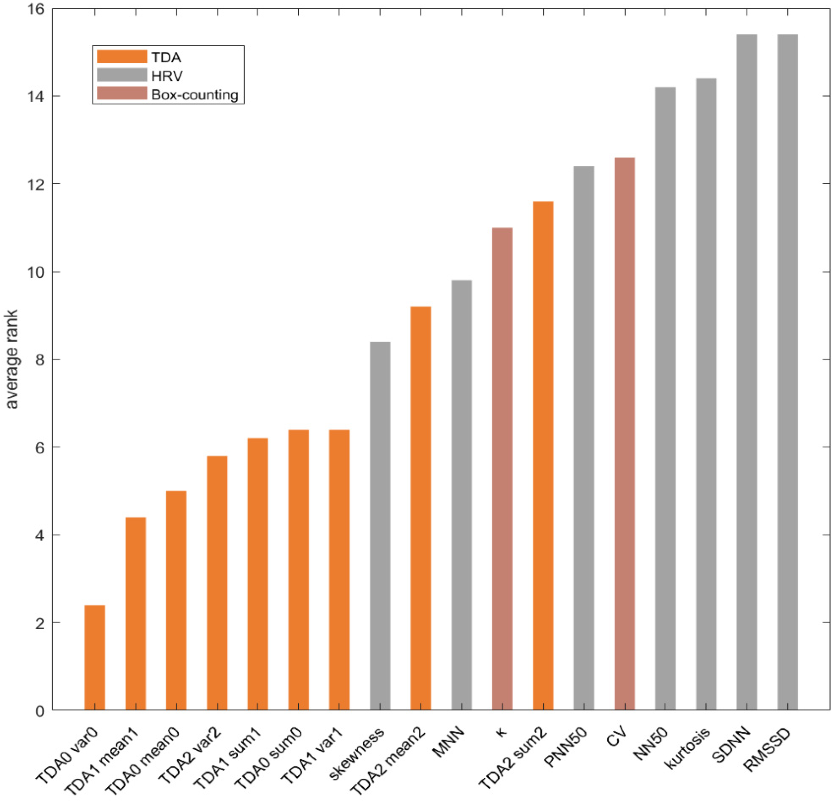
3.4. Features Ranking

In order to verify the characterization performance of the proposed TDA features, we applied five features selection methods (MI, chi-square tests, minimum redundancy maximum relevance (MRMR), out-of-bag predictor for RF, and ReliefF algorithm) to rank the three types of features. Among them, MI method uses MI values to measure the correlation between the features [35]. Chi-square tests rank features using the p-values of the statistics [36]. MRMR method minimizes the redundancy of the feature set and maximizes the relevance of the feature set to the response variable [37,38]. Out-of-bag method measures the influence of the features on the prediction results [39,40,41]. The ReliefF algorithm finds the appropriate weight for each feature through the reward and penal mechanism [42,43,44].

Table 6. Predictor importance scores for five features selection methods.

Features	MI	Chi−Square	MRMR	Out-of-Bag	ReliefF
$\mathrm{TDA}0\_\mathrm{sum}0$	−0.06973	8.52156	0.14073	0.35355	0.22132
$\mathrm{TDA}1\_\mathrm{sum}1$	−0.05626	9.05480	0.16236	0.38521	0.26416
$\mathrm{TDA}2\_\mathrm{sum}2$	−0.26306	1.10083	0.05174	0.06355	−0.04202
$\mathrm{TDA}0\_\mathrm{var}0$	−0.02478	12.90666	0.36806	0.70518	0.58501
$\mathrm{TDA}1\_\mathrm{var}1$	−0.08660	4.96328	0.13049	0.29902	0.20516
$\mathrm{TDA}2\_\mathrm{var}2$	−0.05625	10.68233	0.26268	0.48215	0.26509
$\mathrm{TDA}1\_\mathrm{mean}1$	−0.03002	11.78756	0.29908	0.62190	0.40754
$\mathrm{TDA}2\_\mathrm{mean}2$	−0.12454	1.84986	0.12685	0.17107	0.12099
$MNN$	−0.13324	1.77568	0.10477	0.14286	0.08333
$SDNN$	−0.39715	0.18215	0.00018	−0.14286	−0.14500
$RMSSD$	−0.83429	0.06164	3.49049 × 10−15	−0.14286	−0.15243
$NN50$	−0.31335	0.76527	0.00076	−0.10643	−0.12677
$PNN50$	−0.27056	1.06271	0.04106	0.00000	−0.07877
$kurtosis$	−0.31891	0.39783	0.00071	−0.14286	−0.13620
$skewness$	−0.09189	2.35361	0.13049	0.24026	0.13275
$CV$	−0.27523	1.03846	0.02133	−0.03349	−0.09768
$\kappa$	−0.13934	1.15556	0.05641	0.09654	0.07217

Where $m$ is 6, $\tau$ is 12, and split frame length is 5 s.

shows the predictor importance scores of each feature for each method.

Since each method yielded a different range of predicted impact scores, all features were ranked in each method based on Table 6. For each feature, the average of its five ranking values in the different methods was calculated; the average ranking of each feature is shown in order in Figure 7.

From Figure 7, the TDA features appear, generally, in higher-ranking positions, indicating that the characterization performance of the proposed features is superior than that of the other two previous features.

4. Discussion

4.1. Effect of Reconstruction Parameters and Split Frame Length

In the TDA features extraction workflow, PSR was applied to obtain the point cloud. The reconstruction parameters of PSR are proved to have a great influence on the ability of the point cloud to characterize the intrinsic properties of the original system. In previous approaches, the reconstruction parameters were mostly selected empirically, lacking theoretical support and generalizability. In this study, we compared the effects of the reconstruction parameters $m$ and $\tau$ on the performance of ECG-based VF prediction. In Figure 5, for each split frame length, the distribution of all $\tau$ values tend to spread gradually from the first to the fifth local minimum, indicating that the MI of the original sequence and its time-delayed sequence are gradually increasing. Therefore, the first local minimum was selected to reduce correlation between the two sequences. From inspecting Figure 6, choosing $m=6$ as the minimum embedding dimension enabled over 80% of the data to be sufficiently embedded without causing a large computational burden. It can be seen that the choice of reconstruction parameters directly affects the efficacy of the point cloud and the characterization ability of the TDA features, which is an essential part of VF prediction.

In addition, the effect of the split frame length on the prediction results is discussed, with results demonstrated in Table 4. A trend can be seen in the accuracy results obtained from the classification at different split frame lengths with $\tau$. For both alternative $\tau$ values, the accuracy decreases gradually with increasing split frame lengths. This suggests a possibility of a latent selectivity of TDA for the size of the point cloud. It means that for point clouds reconstructed from ECG signals, if the split frame length is short and, thus, the point cloud is small, then, TDA features are more sensitive to the imminent onset of VF. As the split frame lengths become longer, information about VF is gradually obscured.

4.2. Evaluation of TDA Features

To evaluate the performance of the TDA features, we ranked the entire 18 features using five features selection methods in this work. As shown in Table 6, it can be seen that the TDA features achieve high rankings under various selection methods. In Figure 7, the first seven average rankings are all from TDA features, which indicates that TDA features have an obvious advantage over both HRV features and box-counting features. This may be a result of the fact that the TDA method is able to capture potential details in the time sequence and, together with PSR, can derive the information embedded in the system corresponding to the original signal. For the box-counting features, which are also based on PSR, the characterization ability is limited because of the insufficient reconstruction dimension. Moreover, the HRV features only analyze the information contained in the heartbeat itself, excluding the information of the system contained in the original signal, causing it to get ranked at lower positions. However, the HRV feature $skewness$ achieved the highest ranking behind the TDA features, probably owing to its ability to represent changes in heartbeat rhythm patterns before the onset of VF. In addition, as shown in Table 5, the TDA features achieved the best classification accuracy, which also proves the advantage of the proposed features.

4.3. Comparison with Previous Prediction Methods

Previous ECG-based VF prediction methods were compared, and databases, features, and prediction performance corresponding to the selected literature are listed in

Table 7. List of studies on the ECG-based VF prediction.

Reference Index	Forecast Time	Database	Split Frame Length	ECG Features	Prediction Performance
[4]	15 min	NSRDB 9 VFDB 9	60 s	12 morphological features	Sensitivity 95% Specificity 90%
[5]	13 min	SDDB 23 NSRDB 18	60 s	23 HRV features	Accuracy 84.28%
[6]	30 s	CUDB 27 PAFDB 22 NSRDB 6	120 s	4 QRS features	Accuracy 98.6%
[7]	10 s	MVTDB 78	5 min	11 HRV features	Accuracy 92.2%
[8]	5 min	SDDB 20 NSRDB 18	60 s	13 HRV features	Accuracy 95%
[9]	4 min 31 s	CUDB 32 PTBDB 32	10 heart beats	2 box-counting features	Accuracy 98.44%
[12]	0 s	CUDB 29 MVTDB 30 +29 PAFDB 12 NSRDB 18	20 s	5 HRV features	Accuracy 88.64%
Our work	5 min	CUDB 15 SDDB 15 PTBDB 30	5 s,8 s,10 s,15 s	2 box-counting features 9 TDA features 7 HRV features	Accuracy 95%

.

In terms of the data volume and databases used, 60 ECG records from three databases were used for our study. Among the listed literature, only Joo et al. [7] and Jeong et al. [12] employ a larger amount of data, but both exhibit limitations in the length of forecast time, meaning that the predictions are too close to the onset of VF to provide an advantage in early prediction. In terms of forecast time, we predict VF 5 min before the onset. Studies conducted by Ebrahimzadeh et al. [5] and Mandala et al. [4] achieved longer forecast times, but both are limited by the small data volume. Also, the lack of diversity in databases makes the generalizability of the methods challenging, while the accuracy is lower than our proposed method. For the prediction performance, Khazaei et al. [8], Heng et al. [9], and Taye et al. [6] achieve higher accuracy. However, the forecast time proposed by [6] is very close to the onset of VF. Although [8] is close to our work in terms of forecast time and accuracy, it uses a smaller amount of data from only two public databases, making the prediction result limited by the data. Compared to [9], we advance the forecast time by half a minute while guaranteeing the prediction accuracy, which proves the advantage of this work in relation to early VF prediction.

5. Conclusions

This study sets out to find a new feature for early VF prediction with enhanced performance. The proposed TDA features provide a new perspective on cardiac activity based on nonlinear dynamics. Experimental results indicate that the proposed features effectively improve the accuracy in the field of medium length VF prediction. The proposed features have the potential to be used in the diagnosis of other cardiac diseases. However, the amount of data in the databases used for this study is limited, which will be supplemented with more ECG-based VF databases in future works. Moreover, the elimination of differences among databases needs to be investigated. This will offer the possibility to predict VF earlier with guaranteed accuracy.

References

1. Zipes, D.P.; Wellen, H. Sudden Cardiac Death. Circulation 1998, 98, 2334–2351. [Google Scholar] [CrossRef] [PubMed]
2. Bezzina, C.R.; Priori, S.G. Genetics of sudden cardiac death. Circ. Res. 2015, 116, 1919–1936. [Google Scholar] [CrossRef] [PubMed]
3. Tseng, L.M.; Tseng, V.S. Predicting Ventricular Fibrillation Through Deep Learning. IEEE Access 2020, 8, 221886–221896. [Google Scholar] [CrossRef]
4. Mandala, S.; Senar, M.S. ECG-based prediction algorithm for imminent malignant ventricular arrhythmias using decision tree. PLoS ONE 2020, 15, e0231635. [Google Scholar]
5. Eeab, C.; Af, D. An optimal strategy for prediction of sudden cardiac death through a pioneering feature-selection approach from HRV signal. Comput. Methods Programs Biomed. 2019, 169, 19–36. [Google Scholar]
6. Taye, G.T.; Shim, E.B. Machine learning approach to predict ventricular fibrillation based on QRS complex shape. Front. Physiol. 2019, 10, 1193. [Google Scholar] [CrossRef] [PubMed] [Green Version]
7. Joo, S.; Choi, K.J. Prediction of spontaneous ventricular tachyarrhythmia by an artificial neural network using parameters gleaned from short-term heart rate variability. Expert Syst. Appl. 2012, 39, 3862–3866. [Google Scholar] [CrossRef]
8. Mohammad, K.; Khadijeh, R. Early detection of sudden cardiac death using nonlinear analysis of heart rate variability. Biocybern. Biomed. Eng. 2018, 38, 931–940. [Google Scholar]
9. Heng, W.W.; Ming, E.S.L. Investigating Phase Space Reconstruction of ECG for Prediction of Malignant Ventricular Arrhythmia. Int. J. Integr. Eng. 2020, 12, 187–196. [Google Scholar]
10. Mandal, S.; Mondal, P. Detection of Ventricular Arrhythmia by using Heart rate variability signal and ECG beat image. Biomed. Signal Process. Control 2021, 68, 102692. [Google Scholar] [CrossRef]
11. Sessa, F.; Anna, V. Heart Rate Variability as predictive factor for Sudden Cardiac Death. Aging 2018, 10, 166–177. [Google Scholar] [CrossRef] [Green Version]
12. Jeong, D.U.; Taye, G.T. Optimal length of heart rate variability data and forecasting time for ventricular fibrillation prediction using machine learning. Comput. Math. Methods Med. 2021, 2021, 6663996. [Google Scholar] [CrossRef]
13. Bassareo, P.P.; Mercuro, G. QRS complex enlargement as a predictor of ventricular arrhythmias in patients affected by surgically treated tetralogy of Fallot: A comprehensive literature review and historical overview. Int. Sch. Res. Not. 2013, 2013, 782508. [Google Scholar] [CrossRef]
14. Riasi, A.; Mohebbi, M. Prediction of ventricular tachycardia using morphological features of ECG signal. In Proceedings of the International Symposium on Artificial Intelligence & Signal Processing, Mashhad, Iran, 3–5 March 2015. [Google Scholar]
15. Fojt, O.; Holcik, J. Applying nonlinear dynamics to ECG signal processing. IEEE Eng. Med. Biol. Mag. 1998, 17, 96–101. [Google Scholar] [CrossRef]
16. Small, M. Applied Nonlinear Time Series Analysis: Applications in Physics, Physiology and Finance; World Scientific: Singapore, 2005. [Google Scholar]
17. Amann, A.; Tratnig, R. Detecting Ventricular Fibrillation by Time-Delay Methods. IEEE Trans. Biomed. Eng. 2007, 54, 174–177. [Google Scholar] [CrossRef]
18. Cappiello, G.; Das, S. A Statistical Index for Early Diagnosis of Ventricular Arrhythmia from the Trend Analysis of ECG Phase-portraits. Physiol. Meas. 2014, 36, 107. [Google Scholar] [CrossRef] [Green Version]
19. Koulaouzidis, G.; Das, S. Prompt and accurate diagnosis of ventricular arrhythmias with a novel index based on phase space reconstruction of ECG. Int. J. Cardiol. 2015, 182, 38–43. [Google Scholar] [CrossRef] [Green Version]
20. Roopaei, M.; Boostani, R. Chaotic based reconstructed phase space features for detecting ventricular fibrillation. Biomed. Signal Process. Control 2010, 5, 318–327. [Google Scholar] [CrossRef]
21. Nolle, F.M.; Badura, F.K.; Catlett, J.M.; Bowser, R.W.; Sketch, M.H. CREI-GARD, a new concept in computerized arrhythmia monitoring systems. Comput. Cardiol. 1986, 13, 515–518. [Google Scholar]
22. Greenwald, S.D. Development and Analysis of a Ventricular Fibrillation Detector. Master’s Thesis, MIT Dept of Electrical Engineering and Computer Science, Cambridge, MA, USA, 1986. [Google Scholar]
23. Bousseljot, R.; Kreiseler, D. Use of the ECG signal database CARDIODAT of PTB via the Internet. Biomed. Tech. 1995, 40, 317–318. [Google Scholar]
24. Takens, F. Detecting strange attractors in turbulence. In Dynamical Systems and Turbulence, Warwick, 1980; Springer: Berlin/Heidelberg, Germany, 1981; pp. 366–381. [Google Scholar]
25. Packard, N.H.; Crutchfield, J.P. Geometry from a Time Series. Phys. Rev. Lett. 2008, 45, 712. [Google Scholar] [CrossRef]
26. Abarbanel, H.D.; Brown, R. The analysis of observed chaotic data in physical systems. Rev. Mod. Phys. 1993, 65, 1331. [Google Scholar] [CrossRef] [Green Version]
27. Fraser, A.M.; Swinney, H.L. Independent coordinates for strange attractors from mutual information. Phys. Rev. A 1986, 33, 1134. [Google Scholar] [CrossRef]
28. Rosenstein, M.T.; Collins, J.J. Reconstruction expansion as a geometry-based framework for choosing proper delay times. Phys. D Nonlinear Phenom. 1994, 73, 82–98. [Google Scholar] [CrossRef]
29. Broomhead, D.S.; King, G.P. Extracting qualitative dynamics from experimental data. Phys. D Nonlinear Phenom. 1986, 20, 217–236. [Google Scholar] [CrossRef]
30. Kennel, M.B.; Brown, R. Determining embedding dimension for phase-space reconstruction using a geometrical construction. Phys. Rev. A 1992, 45, 3403–3411. [Google Scholar] [CrossRef]
31. Bukkuri, A.; Andor, N. Applications of Topological Data Analysis in Oncology. Front. Artif. Intell. 2021, 4, 38. [Google Scholar] [CrossRef]
32. Safarbali, B.; Golpayegani, S.M.R.H. Nonlinear dynamic approaches to identify atrial fibrillation progression based on topological methods. Biomed. Signal Process. Control 2019, 53, 101563. [Google Scholar] [CrossRef]
33. Dey, T.K.; Shi, D. SimBa: An Efficient Tool for Approximating Rips-Filtration Persistence via Simplicial Batch-Collapse. J. Exp. Algorithm. (JEA) 2019, 24, 1–16. [Google Scholar] [CrossRef] [Green Version]
34. Kantz, H.; Schreiber, T. Nonlinear Time Series Analysis; Cambridge University Press: Cambridge, UK, 2004. [Google Scholar]
35. Battiti, R. Using mutual information for selecting features in supervised neural net learning. IEEE Trans. Neural Netw. 1994, 5, 537–550. [Google Scholar] [CrossRef] [Green Version]
36. Wang, Y.; Zhou, C. Feature selection method based on chi-square test and minimum redundancy. In Proceedings of the International Conference on Intelligent and Interactive Systems and Applications, Shanghai, China, 25–27 September 2020. [Google Scholar]
37. Ding, C. Minimum redundancy feature selection from microarray gene expression data. J. Bioinform. Comput. Biol. 2005, 3, 185–205. [Google Scholar] [CrossRef] [PubMed]
38. Darbellay, G. Estimation of the information by an adaptive partitioning of the observation space. IEEE Trans. Inf. Theory 1999, 45, 1315–1321. [Google Scholar] [CrossRef] [Green Version]
39. Leo, B.; Jerome, H.F.; Richard, A. Classification and Regression Trees, 1st ed.; CRC Press: Boca Raton, FL, USA, 1984. [Google Scholar]
40. Loh, W.Y. Regression Trees with Unbiased Variable Selection and Interaction Detection. Stat. Sin. 2002, 12, 361–386. [Google Scholar]
41. Loh, W.Y. Split Selection Methods for Classification Trees. Stat. Sin. 1997, 7, 815–840. [Google Scholar]
42. Kononenko, I.; Šimec, E. Overcoming the myopia of inductive learning algorithms with RELIEFF. Appl. Intell. 1997, 7, 39–55. [Google Scholar] [CrossRef]
43. Robnik-Šikonja, M.; Kononenko, I. An adaptation of Relief for attribute estimation in regression. In Proceedings of the Fourteenth International Conference on Machine Learning, Nashville, TN, USA, 8–12 July 1997. [Google Scholar]
44. Robnik-Šikonja, M.; Kononenko, I. Theoretical and empirical analysis of ReliefF and RReliefF. Mach. Learn. 2003, 53, 23–69. [Google Scholar] [CrossRef]
Figure 1. Workflow of the proposed method for prediction of VF.
Applsci 12 10370 g001
Figure 2. Results of pre-processing. (a) The original ECG signal; (b) The pre-processed ECG signal. By comparison, the baseline drift in the original ECG signal is eliminated by moving average filtering and its amplitude is adjusted to the 0–1 range by normalization.
Applsci 12 10370 g002
Figure 3. Phase space trajectories of VF and nVF split frames. (a) VF split frame; (b) nVF split frame.
Applsci 12 10370 g003
Figure 4. Barcode diagram of VF and nVF split frames. (a) VF split frame with Betti number 0 to 2; (b) nVF split frame with Betti number 0 to 2.
Applsci 12 10370 g004
Figure 5. Box plots for four different split frame lengths. (a) 5s-length split frame: the median of the first local minimum of the MI function is obtained as 12; (b) 8s-length split frame: the median of the first local minimum is 10.5; (c) 10s-length split frame: the median of the first local minimum is 12.5; (d) 15s-length split frame: the median of the first local minimum is 11. And the “+” represents the outlier.
Applsci 12 10370 g005
Figure 6. Probability density curve of the embedding dimension.
Applsci 12 10370 g006
Figure 7. Average rank of each feature.
Applsci 12 10370 g007