Kerr-Lens Mode-Locking: Numerical Simulation of the Spatio-Temporal Dynamics on All Time Scales

Abstract

We present a complete numerical analysis and simulation of the full spatio-temporal dynamics of Kerr-lens mode-locking in a laser. This dynamic, which is the workhorse mechanism for generating ultrashort pulses, relies on the intricate coupling between the spatial nonlinear propagation and the temporal nonlinear compression. Our numerical tool emulates the dynamical evolution of the optical field in the cavity on all time-scales: the fast time scale of the pulse envelope within a single round trip, and the slow time-scale between round-trips. We employ a nonlinear ABCD formalism that fully handles all relevant effects in the laser, namely—self focusing and diffraction, dispersion and self-phase modulation, and space-dependent loss and gain saturation. We confirm the validity of our model by reproducing the pulse-formation in all aspects: The evolution of the pulse energy, duration, and gain during the entire cavity buildup, demonstrating the nonlinear mode competition in full, as well as the dependence of the final pulse in steady state on the interplay between gain bandwidth, dispersion, and self-phase modulation. The direct observation of the nonlinear evolution of the pulse in space-time is a key enabler to analyze and optimize the Kerr-lens mode-locking operation, as well as to explore new nonlinear phenomena.

1. Introduction

Kerr-lens mode-locking (KLM) is a state-of-the-art technique for generating ultrafast pulses, central to the field of ultrafast lasers and is extensively used [1,2,3]. KLM relies on the highly non-linear interplay between the spatial and temporal properties of the field inside the laser cavity that is challenging to fully analyze [4,5,6] and, in many cases, requires approximations that exclude some of the intricacies of these oscillators. As a result, the design of KLM-based oscillators often relies strongly on intuition and trial-error experience. Most standard methods of analysis focus on the steady-state of the field [2,7,8,9,10,11,12,13], but cannot describe the dynamical evolution towards this steady state. Some other methods make different approximations to separate the spatial and temporal parts of the dynamics [14], which is effective for understanding the basic operation of KLM lasers, but can miss important dynamics in the interplay between the spatial and temporal profiles of the field [15].

We introduce a numerical simulation algorithm, along with an open-source MATLAB program that calculates from first principles the complete dynamics of the spatio-temporal field profile in a KLM oscillator for a wide range of operation regimes. Our method is able to reproduce the evolution of the field in both space and time—starting from an initial noise-seed up to steady-state pulses. The only assumption being made is that the spatial beam of the laser is a single mode, well approximated by a Gaussian profile. This is a practically universal regime of operation in KLM lasers that are strongly driven to a single spatial mode by the interaction between the self-focusing Kerr-lensing and the diffraction through the effective aperture in the cavity [2,3].

Our paper is structured as follows: Section 2 includes the major validations, where the simulation reconstructs fundamental properties of KLM oscillators—soliton formation from spontaneous noise and its dependence on the laser parameters, such as gain bandwidth, gain saturation, self-phase modulation (SPM), linear and nonlinear dispersion, all from first principles. This section also shows how different pulse properties depend delicately on the spatial cavity parameters and how we can use the full simulation of a KLM laser to assist cavity design. Section 3 provides a detailed description of the paradigm of our numerical simulation and the algorithm.

2. Results

Before we delve into the intricacies of the algorithm of the numerical simulation, let us demonstrate the performance of the simulation by reconstructing the complete dynamical evolution of the pulse, from the initial spontaneous noise seed, through the entire cavity buildup, to the final steady state. We will show how the spatial mode of the cavity is formed in steady state by self-focusing and how the soliton pulse is dictated by the interplay between gain-bandwidth, dispersion, and SPM.

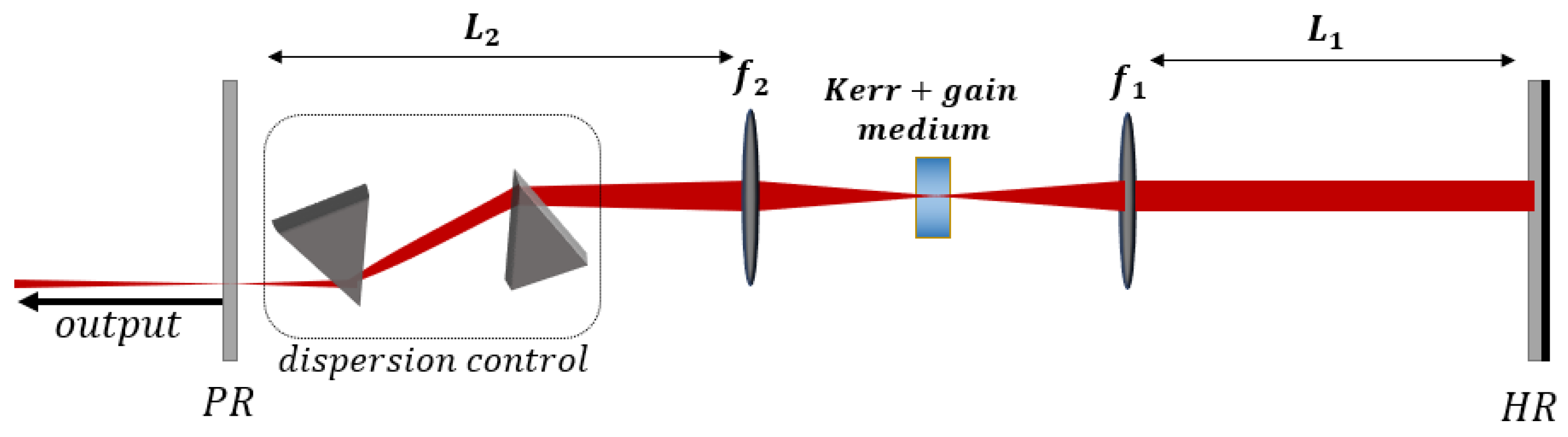
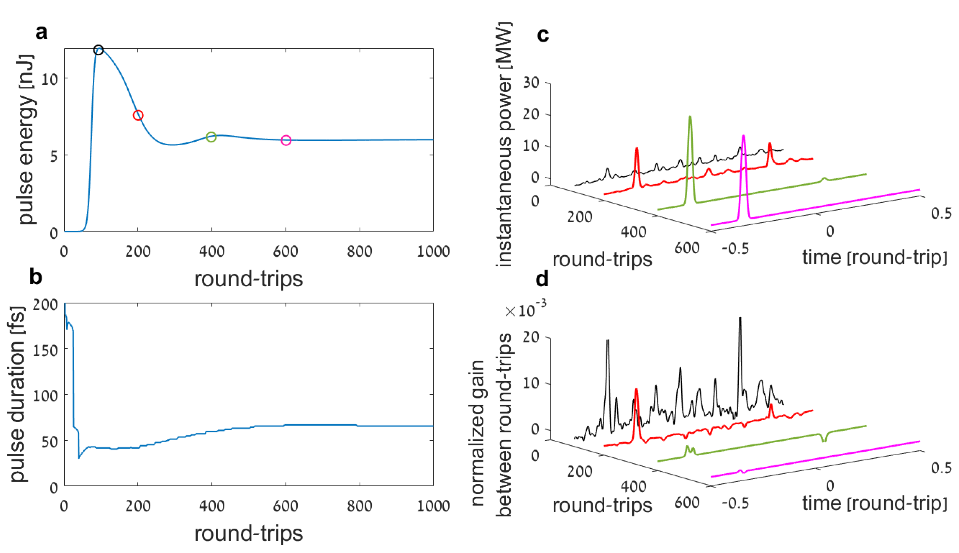
The simulation assumes the standard linear cavity layout of Figure 1, and the evolution of the intra-cavity field during the laser buildup is highlighted in Figure 2. The cavity (pulse) energy (Figure 2a) and the pulse-duration (FWHM, Figure 2b) are shown as a function of round-trip number (the slow time scale), where three stages of evolution are evident (I) the initial exponential growth, (II) the nonlinear mode competition, and (III) the final steady-state. To understand the dynamical operation during each stage, we sampled four specific round-trips from the different stages, which are shown in Figure 2c (instantaneous power) and Figure 2d (instantaneous power gain) as a function of time within a single round-trip (fast time scale). The colors of the graphs in Figure 2c,d correspond to the circles on the energy graph of Figure 2a. The field at the end of the initial exponential growth (black) is highly noisy and multi-pulsed, with noisy, yet positive gain at all times. This picture changes during the mode competition (red and green). We observe a number of pulses competing for the gain, before all pulses, except one, diminish. During that phase, we also observe variations in the shape of the main pulse. Finally, the purple graph shows the stable pulse near steady state.

It is worth noting that our simulated cavity shows a self-starting mode-lock dynamic under suitable conditions, with no special starting mechanism. This is due to the assumption of ideally slow gain saturation, which is calculated only over the slow time scale of cavity round-trips. Specifically, we assume that the gain within each round trip depends only on the total energy of that round-trip, not to be influenced by the temporal profile of the field within the round trip. Thus, a noise seed at the first round trip will basically grow undisturbed and maintain its temporal profile until the Kerr effect kicks in to favor one specific temporal fluctuation (usually the highest one) to form a single pulse. Although this assumption of slow gain saturation is well validated for the Ti:Sapphire gain medium with ultrashort pulses, it is not correct for a continuous field, where the finite memory of the gain saturation leads to relaxation oscillations and slow damping of temporal fluctuations. Consequently, an external noise mechanism may be needed in reality to induce sufficiently large fluctuations to enjoy the benefit of the Kerr-lens before they are damped out by the gain dynamics.

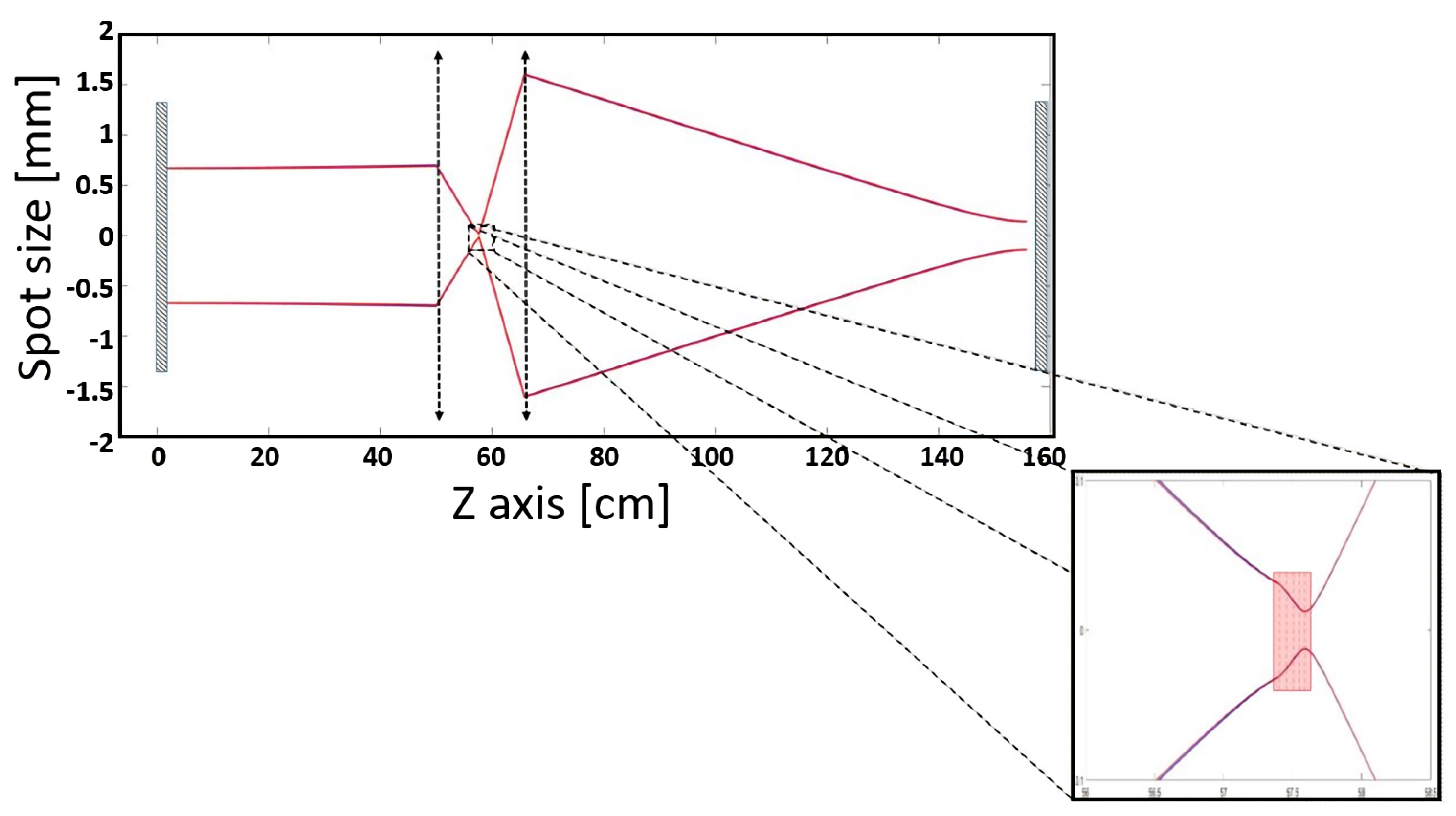
Our simulation is fully spatio-temporal, and calculates the beam propagation through the cavity in space as well as in time. Figure 3 shows the propagation of the beam through a single run of the cavity. The core function of the Kerr-lens is shown in the inset, where the simulation captures the lensing effect that creates an effective “wave-guide” that stabilizes the cavity and counteracts the diffraction losses.

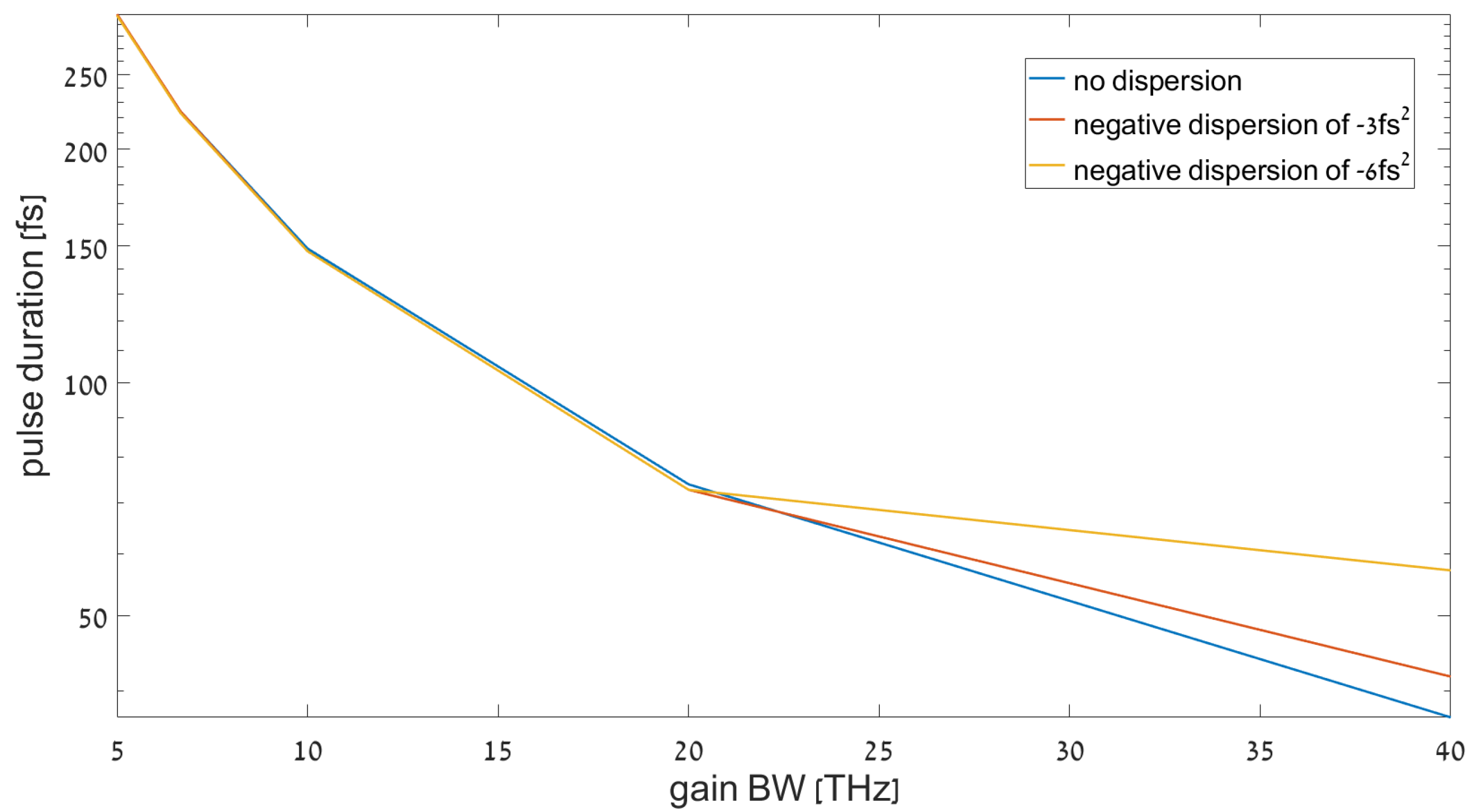
The temporal width of the pulse is dictated by the gain bandwidth and the chromatic dispersion (GVD). The gain-bandwidth sets a lower bound on the pulse duration (by Fourier uncertainty), and the dispersion distorts the temporal shape of the pulse (chirping), which affects shorter pulses more severely than longer pulses [16]. Thus, the net GVD of the cavity sets another lower bound on the pulse-duration. Our simulation correctly reproduces this behavior, as shown in Figure 4, where the pulse duration follows the gain bandwidth limit until it reaches the dispersion limit.

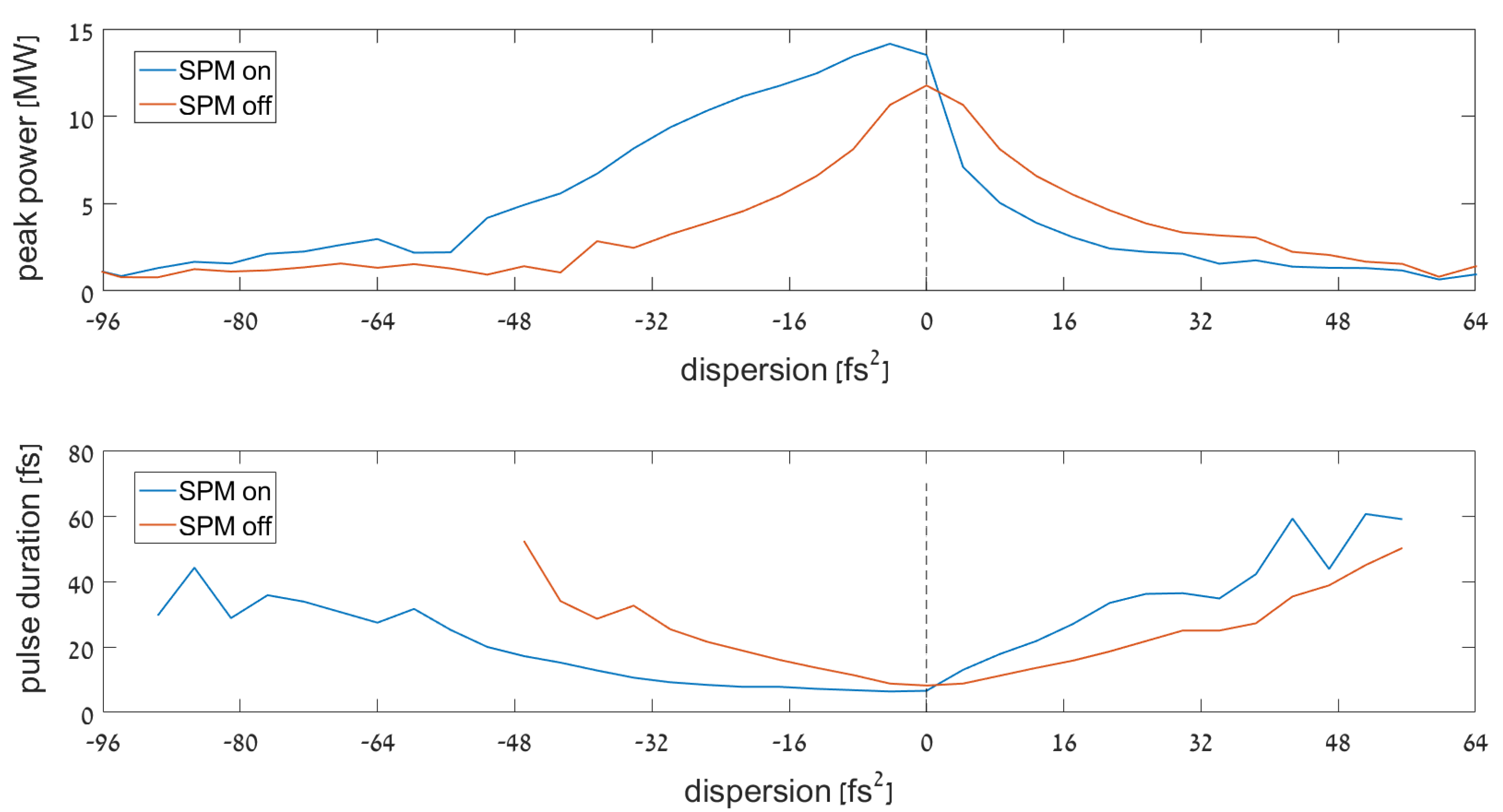
So far, we considered only linear effects on the pulse duration due to GVD and gain bandwidth. The pulse, however, is highly affected by the nonlinear chirping due to SPM, which is critical in the soliton formation mechanism. Specifically, SPM chirping acts as another source of dispersion that shifts the optimal GVD value toward a small negative value. Interestingly, the simulation can explore this interplay between SPM and GVD in greater detail than possible in the experiment. Specifically, in the simulation, we can simply turn off the temporal SPM effects, while keeping the spatial Kerr-lensing effect, and compare the pulse performance in this (unphysical) situation to the one with SPM, a feat that is inherently impossible in the experiment. Figure 5 highlights exactly this comparison: we plot the pulse duration as a function of the linear GVD in the cavity with SPM (blue) and without (orange). Indeed, the simulation shows that SPM shifts the optimal pulse formation toward the negative GVD range as expected, but also that SPM enhances the peak power at the optimal GVD value. Thus, optimal operation is achieved at some dispersion, rather than the zero dispersion point.

Beyond the validations presented above, this simulation already served two previous publications, where it was used to predict and analyze new details of KLM, with quantitative agreement with experimental results. Specifically, in [15], we used the simulation to observe and explore the effective saturable-absorption mechanism of KLM, where, although no actual absorption takes place, there are diffraction losses over an effective aperture form the saturation loss mechanism. Using the simulation, we identified how and where exactly these losses occur, which aided us to experimentally measure this time-dependent loss for the first time. In another paper [17], we used the simulation to show that KLM lasers can break the spatial symmetry between the forward and backward halves of the round-trip in a linear cavity when the pump power is increased above the mode-locking threshold. This symmetry breaking allows the laser to increase the energy of the pulse. Both of these phenomena would have been impossible to predict without a full dynamical simulation, which illustrates the utility of this numerical tool.

3. Materials and Methods

The simulation assumes a set of common parameter values for the cavity configuration, gain medium and Kerr medium, that are typical for KLM experiments [18,19]. The values used in the simulation appear in

Table 1. Parameter values for the cavity configuration and the Kerr medium.

Parameter	Value
NL refractive index—$n_2$	$3\times {10}^{-16}$ cm${}^2$/W
Kerr (gain) medium thickness—$L_c$	3 mm
Length of short arm—$L_1$	50 cm
Length of long arm—$L_2$	90 cm
Focus of cavity lenses/mirrors—f	75 mm
pump waist in gain medium—$w_p$	30 $\mathsf{\mu }$m

.

Our simulation focuses on KLM oscillators in a single transverse spatial-mode, which is time-dependent due to the Kerr-lens.

$$E(r,z,t)=A_s(r,z)A_t(t,\tau )$$

(1)

where $A_s(r,z)$ is a transverse Gaussian–Hermite mode and $A_t(t,\tau )$ is a slowly-varying time dependent envelope that we divide into two time-scales, as shown in Figure 6. This product separation of space and time is justified on two accounts—(1) the oscillation spectrum is relatively small compared to the carrier frequency (for pulses down to  10 fs or so), indicating that spectral variations are small; (2) The Kerr-lens, which dominates the dynamics on the fast time scale, acts instantaneously without memory, which corresponds to a very weak (nearly non-existent) frequency dependence. Furthermore, the approximation that the spatial profile is a single transverse Gaussian mode is justified since the nonlinear losses strongly drive the laser toward a single, high-intensity spatial beam. Generally, this approximation is only correct for paraxial propagation, which is well justified for the small divergence angles of the optical beams in our simulation cavity. Aberrations of the Kerr-lens can, in principle, couple energy into higher spatial-modes; however, these aberrations do not build up in the cavity, but rather lead to diffraction outside the cavity, which is encapsulated in the total diffraction loss term.

KLM oscillators can be thought of as passive cavities, with an intensity-dependent lens (or lenses) that couples the temporal and spatial dynamics. When the diffraction losses are also included, the Kerr-lensing effect generates an effective saturable absorber with an instantaneous response, able to generate extremely short pulses [4,20,21,22]. As such, the KLM oscillator can be divided conceptually into two parts—linear and non-linear. The linear part accounts for the gain spectrum and saturation, dispersion, and linear loss, which can be encapsulated into a total spectral transfer function:

$$E\left(\omega \right)\to g\left(\omega \right)T\left(\omega \right)E\left(\omega \right),$$

(2)

where $g\left(\omega \right)$ is the spectral gain of the active medium and $T\left(\omega \right)$ is the transfer function of the passive elements in the cavity. The spectral phase of $T\left(\omega \right)$ reflects the chromatic dispersion and its amplitude reflects the cavity loss ${\parallel T\parallel }^2=1-\mathrm{loss}$.

To take into account the gain depletion, which leads to non-linear saturation and mode competition, we reduce the gain $g\left(\omega \right)$ as the intra-cavity pulse energy U increases according to the standard saturation formula,

$$g\left(\omega \right)=\frac{g_0\left(\omega \right)}{1+U/U_{\mathrm{sat}}},$$

(3)

where $U_{\mathrm{sat}}$ is the saturation energy of the gain medium, taken to be $\tau ·2.6 \mathrm{W}$ for our simulation ($\tau$ is the round trip time and the saturation power of 2.6 W is based on the saturation intensity of Ti:Sapphire in the literature, calculated for a 3 mm long crystal with $0.25\%$ doping and $20$ μm beam waist for the pump) [23].

We now need to account for the nonlinear response of the Kerr medium, i.e., Kerr-lens and SPM, which we assume to be instantaneous. For simplicity, we start with a thin Kerr medium, whose thickness $L_c$ is much smaller than the Rayleigh beam range $L_c\ll z_R$, and later generalize the result for a thick medium. The ABCD matrix of a thin Kerr medium is a simple lens with an intensity-dependent focus:

$$M_{\mathrm{kl}}\left(t\right)=\left(\begin{array}{cc}1& 0\\ -\frac{1}{f_{kl}\left(t\right)}& 1\end{array}\right)$$

(4)

where $f_{kl}$ is the time dependent Kerr-lens focus, which, for a thin nonlinear medium, is given by:

$$\frac{1}{f_{kl}}=\frac{8n_2{L}_c}{\pi w{\left(t\right)}^2}I\left(t\right),$$

(5)

with $n_2$ the nonlinear index of refraction, $L_c$ the medium length, $w\left(t\right)$ the instantaneous beam waist, and $I\left(t\right)$ the on-axis instantaneous intensity [19]. The SPM of a thin Kerr medium is a simple phase modulation of $e^{i4n_{2}I\left(t\right)L_c/\pi \lambda }$.

This introduces a new, fast time scale t into the problem. Unlike the slow laser dynamics, which occur on a time scale of many round-trips (from one round-trip to the next), the instantaneous Kerr-lens evolves on the pulse time-scale within a single cavity round-trip. As a result, we use two different time variables to describe the cavity dynamics—n, which enumerates the round-trip time, and a fast time variable t, which measures the time within each round-trip.

The beam, under the Gaussian approximation, is completely described by two variables—the instantaneous power $P_n\left(t\right)$ and Gaussian beam parameter $q_n\left(t\right)$ that reflects the beam waist w and phase curvature R as $\frac{1}{q}=\frac{1}{R}-i\frac{\lambda }{\pi w^2\left(t\right)}$. The local intensity is $I_n\left(t\right)=\frac{P_n\left(t\right)}{w^2\left(t\right)}$. With the instantaneous power and beam parameter we can calculate the instantaneous matrix $M_{kl}\left(t\right)$. The total ABCD matrix of the cavity round trip can now be written. For a ring cavity it is,

$$M_{ring}\left(t\right)=M_{cav}{M}_{kl}\left(t\right).$$

(6)

However, for a linear cavity, the Kerr interaction occurs twice, which leads to:

$$M_{lin}\left(t\right)=M_1{M}_{kl}^{+}\left(t\right)M_2{M}_{kl}^{-}\left(t\right),$$

(7)

where $M_{1,2}$ are the linear ABCD matrices for the two halves of the cavity around the Kerr medium and $M_{kl}^{\pm }$ are the nonlinear lens matrices in the forward and backward propagation through the cavity, which are time dependent and not necessarily equal. In fact, the dual interaction with the Kerr medium can break the symmetry between the forward and backwards direction, as we showed in [17]. Note that under a small-gain (or slow-varying envelope) assumption, the order of the cavity elements is not of particular importance, and would not change the results.

For a thick Kerr medium, whose thickness cannot be neglected relative to the Rayleigh range, we must also account for the propagation of the beam within the nonlinear medium. This can be approximated with a split-operator approach, where the thick medium is divided into $N_{kl}$ thin lenses that are separated by a short distance $l=L_c/N_{kl}$ of free propagation. The total matrix of the Kerr medium then becomes:

$$M_{kl}^{thick}\left(t\right)=M_z(l/2)M_{kl}^{\left(1\right)}\left(t\right)M_z\left(l\right)M_{kl}^{\left(2\right)}\left(t\right)···M_z\left(l\right)M_{kl}^{\left(N_{kl}\right)}\left(t\right)M_z(l/2),$$

(8)

where $M_z\left(l\right)$ is the free space matrix and $M_{kl}^{\left(i\right)}\left(t\right)$ are the thin Kerr-lenses of Equation (5), each calculated according to the beam parameter at its location $q^i\left(t\right)$. The thick-lens is factorized this way so that multiplying several thick-lens matrices would give, yet again, a thick-lens. In our simulation, the Kerr medium of thickness $L_c=3$ mm was divided into $N_{kl}=5$ thin lenses.

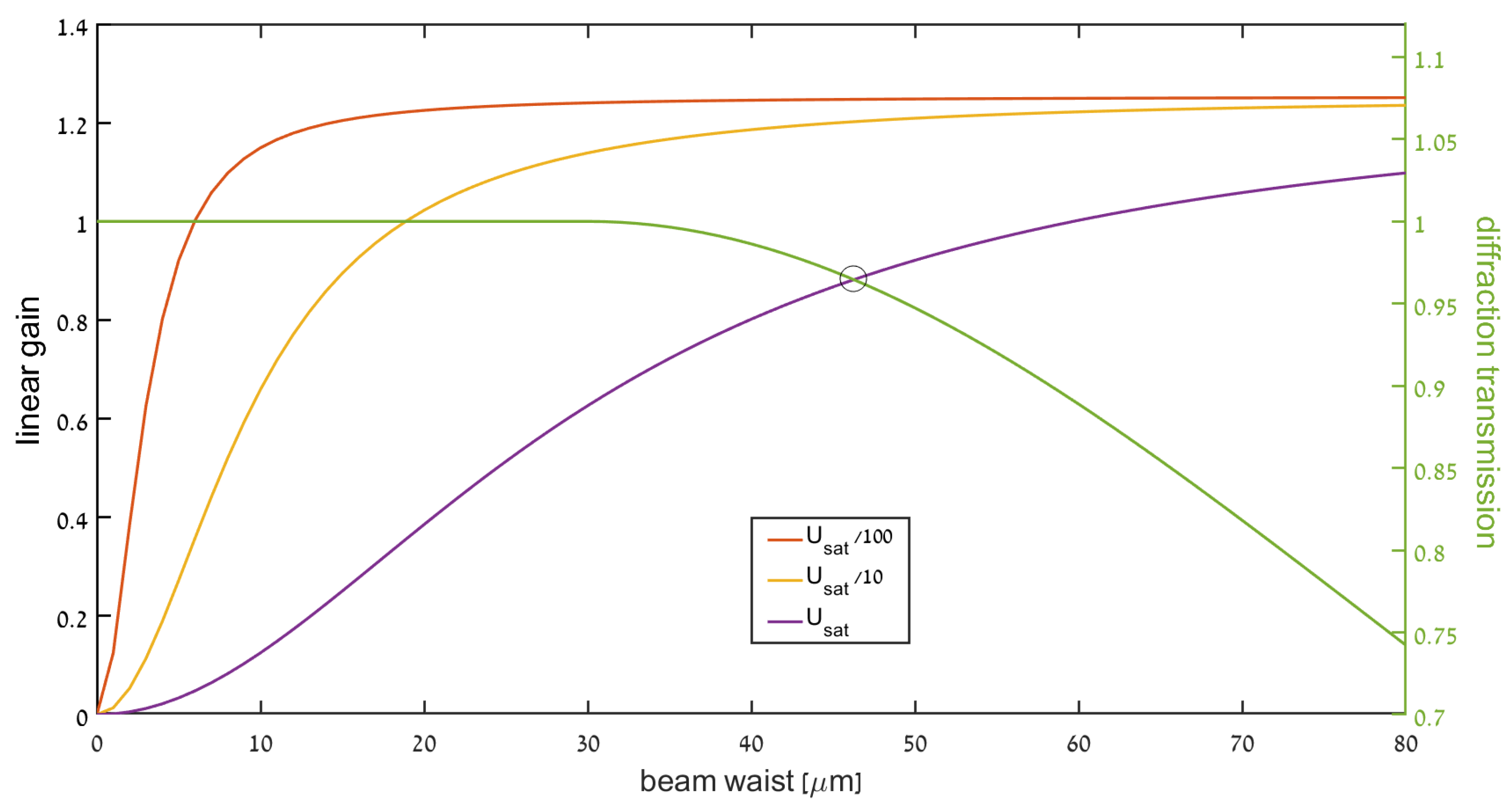
The nonlinear diffraction loss due to the Kerr-lensing effect is at the heart of KLM. In the single-mode regime, the Kerr-lensing effect couples the beam size and the (on-axis) instantaneous intensity at the crystal. Thus, by inserting a mechanism that penalizes the laser for large beams [15,19,24], we can create an effective saturable absorber. Here, we note two competing loss/saturation mechanisms—small beams suffer from insufficient overlap with the pump mode, which reduces their gain, whereas larger beams suffer increased loss due to the effective Kerr lens aperture. This competition is summarized in Figure 7. In general, the nonlinear losses can be divided into two categories: hard apertures, where any power beyond a certain beam size is completely cut off; and soft apertures, where beams beyond a certain size incur a certain amount of loss that depends on the beam’s size [3,10,11]. Both can be easily incorporated into our simulation.

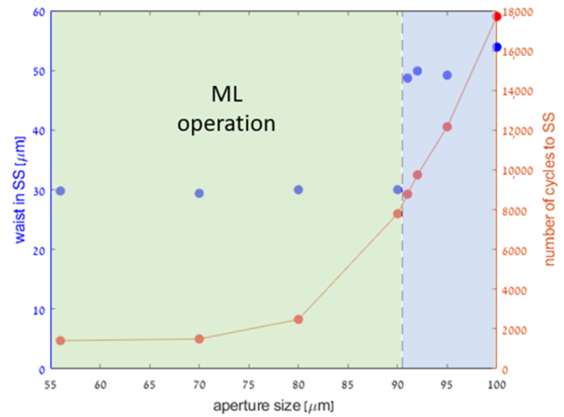
In our simulation, we opt for a soft-aperture mechanism, corresponding to a situation where the most important loss mechanism is the spatial overlap between the laser and the pump mode at the gain medium, where the KLM operates slightly beyond the stability limit. Different mechanisms simply amount to different loss functions, and can be easily accommodated by our software. For numerical reasons, in order to assure convergence of the cavity evolution (power and beam parameter) to the steady state, we need to prevent the beam size from diverging during the initial stage of cavity amplification, when the intra-cavity power is too low to support a significant Kerr lens. For this purpose, we introduce an artificial hard aperture in the round trip that limits the size of large beams effectively without incurring loss on smaller beams. For a narrow beam, only the (exponentially small) wings of the beam would be affected by the aperture and the incurred loss would be minute. This does not affect the dynamics of the cavity or the steady-state value, but only the convergence time of the simulation, as illustrated in Figure 8.

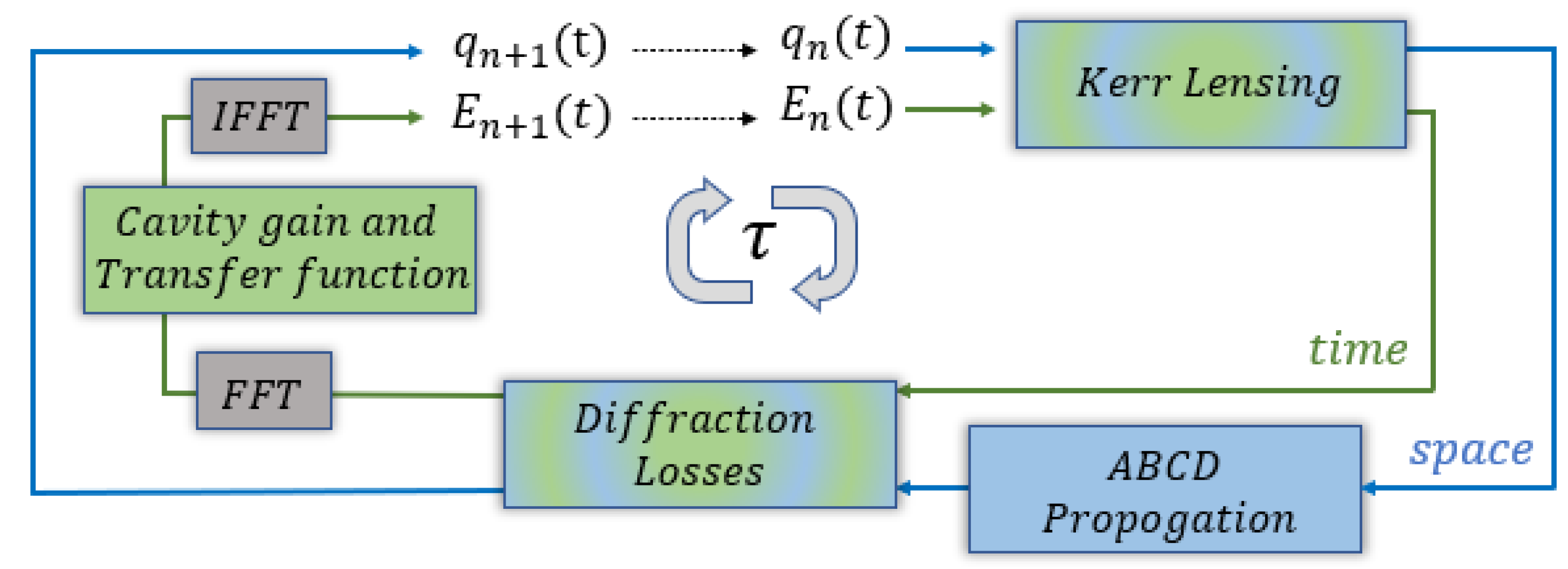
The simulation is performed partially in the time domain, where the instantaneous nonlinear effects are calculated, and partially in the frequency domain where the linear transfer function of the cavity is calculated, as detailed in the pseudo-code given in Algorithm A1. To propagate the field in both time and space, the simulation is divided into a spatial procedure and a temporal procedure. The spatial procedure, detailed in the pseudo-code in Algorithm A2, handles the spatial ABCD propagation under the Gaussian single-mode assumption (including the spatial Kerr and the diffraction losses). The temporal procedure, detailed in the pseudo-code in Algorithm A3, handles the temporal evolution of SPM, gain, loss, and dispersion. The two components are coupled through the Kerr-lens interaction, where the temporal profile of the beam determines the optical power of the Kerr-lens, which, in turn, affects the temporal evolution via the diffraction losses. The variables and function names are given in

Table 2. Variable names and descriptions.

Simulation Parameters	Description
$E\left(t\right)$	Field in time, M-vector.
$\widehat{E}\left(\omega \right)$	Field in frequency, M-vector.
N	Total number of cavity round-trips in the simulation.
M	Total number of time-points within each round-trip.
$w\left(t\right)$	Instantaneous beam waist, M-vector for each round.
$R\left(t\right)$	Beam radius of curvature, M-vector.
$P\left(t\right)$	Beam power, M-vector.
$I\left(t\right)$	Beam intensity at the waist, M-vector.
$q\left(t\right)$	Complex beam radius, M-vector.
$g_0$	Small-signal gain (at center frequency).
$g(\overline{P},w\left(t\right))$	Saturated gain (depends on waist and average power).
$s_0$	Cavity loss rate (at center frequency).
${\sigma }_G$	Gain/loss bandwidth (assuming Lorentzian spectrum).
${\sigma }_D$	Linear dispersion (GVD).
$L_1$	Right cavity arm-length.
$L_2$	Left cavity arm-length.
$L_c$	Crystal’s length.

.

4. Conclusions

We introduced a complete algorithm, accompanied by an open-source MATLAB package for simulating the real-time dynamics of a Kerr-lens mode-locked laser. We simulate from basic principles the complete coupled spatio-temporal dynamics of the laser cavity, under only the assumption of a single Gaussian spatial mode, allowing to observe the complete dynamical evolution of the pulse field in the cavity from the initial noise field to the final steady state. The simulation was thoroughly validated by reproducing all the basic properties of Kerr-lens mode-locked lasers, such as the dependence of the pulse duration in the gain bandwidth, the dispersion, and the self-phase modulation with reasonable agreement to the documented behavior of KLM in Ti:Sapphire. We demonstrate the evolution of pulse energy and duration, as well as the gain dynamics that determine them. Furthermore, the simulation also predicted novel phenomena of space-time coupling in linear KLM cavities [15,17], which demonstrates the power of the simulation as a tool for the design and analysis of ultrafast lasers.

References

1. Herrmann, J. Theory of Kerr-lens mode-locking: Role of self-focusing and radially varying gain. J. Opt. Soc. Am. B 1994, 11, 498–512. [Google Scholar] [CrossRef]
2. Brabec, T.; Spielmann, C.; Curley, P.F.; Krausz, F. Kerr lens mode locking. Opt. Lett. 1992, 17, 1292–1294. [Google Scholar] [CrossRef] [PubMed]
3. Brabec, T.; Schmidt, A.J.; Curley, P.F.; Spielmann, C.; Wintner, E. Hard-aperture Kerr-lens mode locking. J. Opt. Soc. Am. B 1993, 10, 1029–1034. [Google Scholar] [CrossRef]
4. Kurtner, F.X.; der Au, J.A.; Keller, U. Mode-locking with slow and fast saturable absorbers-what’s the difference? IEEE J. Sel. Top. Quantum Electron. 1998, 4, 159–168. [Google Scholar] [CrossRef] [Green Version]
5. Matsko, A.B.; Savchenkov, A.A.; Liang, W.; Ilchenko, V.S.; Seidel, D.; Maleki, L. Mode-locked Kerr frequency combs. Opt. Lett. 2011, 36, 2845. [Google Scholar] [CrossRef] [PubMed]
6. Haus, H.A. Mode-Locking of Lasers. IEEE J. Sel. Top. Quantum Electron. 2000, 6, 1173–1185. [Google Scholar] [CrossRef]
7. Magni, V.; Cerullo, G.; De Silvestri, S. ABCD matrix analysis of propagation of gaussian beams through Kerr media. Opt. Commun. 1993, 96, 348–355. [Google Scholar] [CrossRef]
8. Coen, S.; Randle, H.G.; Sylvestre, T.; Erkintalo, M. Modeling of octave-spanning Kerr frequency combs using a generalized mean-field Lugiato–Lefever model. Opt. Lett. 2012, 38, 37. [Google Scholar] [CrossRef] [Green Version]
9. Salin, F.; Piché, M.; Squier, J. Mode locking of Ti:Al2O3 lasers and self-focusing: A Gaussian approximation. Opt. Lett. 1991, 16, 1674. [Google Scholar] [CrossRef] [PubMed]
10. Lee, Y.W.; Yi, J.H.; Cha, Y.H.; Rhee, Y.J.; Lee, B.C.; Yoo, B.D. Numerical Analysis of Soft-Aperture Kerr-Lens Mode Locking in Ti:Sapphire Laser Cavities by Using Nonlinear ABCD Matrices. J. Korean Phys. Soc. 2005, 46, 1131–1136. [Google Scholar]
11. Juang, D.G.; Chen, Y.C.; Hsu, S.H.; Lin, K.H.; Hsieh, W.F. Differential gain and buildup dynamics of self-starting Kerr lens mode-locked Ti:sapphire laser without an internal aperture. J. Opt. Soc. Am. B 1997, 14, 2116–2121. [Google Scholar] [CrossRef]
12. Cerullo, G.; Silvestri, S.D.; Magni, V. Self-starting Kerr-lens mode locking of a Ti:sapphire laser. Opt. Lett. 1994, 19, 1040–1042. [Google Scholar] [CrossRef] [PubMed]
13. Henrich, B.; Beigang, R. Self-starting Kerr-lens mode locking of a Nd:YAG-laser. Opt. Commun. 1997, 135, 300–304. [Google Scholar] [CrossRef]
14. Sander, M.Y.; Birge, J.; Benedick, A.; Crespo, H.M.; Kärtner, F.X. Dynamics of dispersion managed octave-spanning titanium:sapphire lasers. J. Opt. Soc. Am. B 2009, 26, 743–749. [Google Scholar] [CrossRef]
15. Parshani, I.; Bello, L.; Meller, M.E.; Pe’er, A. Diffractive saturable loss mechanism in Kerr-lens mode-locked lasers: Direct observation and simulation. Opt. Lett. 2021, 46, 1530. [Google Scholar] [CrossRef] [PubMed]
16. Proctor, B.; Westwig, E.; Wise, F. Characterization of a Kerr-lens mode-locked Ti:sapphire laser with positive group-velocity dispersion. Opt. Lett. 1993, 18, 1654–1656. [Google Scholar] [CrossRef] [PubMed]
17. Parshani, I.; Bello, L.; Meller, M.E.; Pe’er, A. Spatial symmetry breaking by non-local Kerr-lensing in mode-locked lasers. arXiv 2021, arXiv:2111.12078. [Google Scholar] [CrossRef]
18. Yefet, S.; Pe’er, A. Mode locking with enhanced nonlinearity—A detailed study. Opt. Express 2013, 21, 19040. [Google Scholar] [CrossRef] [PubMed] [Green Version]
19. Yefet, S.; Pe’er, A. A Review of Cavity Design for Kerr Lens Mode-Locked Solid-State Lasers. Appl. Sci. 2013, 3, 694–724. [Google Scholar] [CrossRef] [Green Version]
20. Kartner, F.; Jung, I.; Keller, U. Soliton mode-locking with saturable absorbers. IEEE J. Sel. Top. Quantum Electron. 1996, 2, 540–556. [Google Scholar] [CrossRef]
21. Haus, H.A. Theory of mode locking with a fast saturable absorber. J. Appl. Phys. 1975, 46, 3049–3058. [Google Scholar] [CrossRef]
22. Chen, C.J.; Wai, P.K.A.; Menyuk, C.R. Self-starting of passively mode-locked lasers with fast saturable absorbers. Opt. Lett. 1995, 20, 350–352. [Google Scholar] [CrossRef] [PubMed]
23. Available online: https://www.rp-photonics.com/saturation_power.html (accessed on 26 September 2022).
24. Wright, L.G.; Sidorenko, P.; Pourbeyram, H.; Ziegler, Z.M.; Isichenko, A.; Malomed, B.A.; Menyuk, C.R.; Christodoulides, D.N.; Wise, F.W. Mechanisms of spatiotemporal mode-locking. Nat. Phys. 2020, 16, 565–570. [Google Scholar] [CrossRef]
25. Idan Parshani, L.B. klm-Sim. 2022. Available online: https://github.com/leonbello/klm-sim (accessed on 26 September 2022).
Figure 1. The cavity layout of a standard KLM laser in a linear cavity: The cavity focus is formed by two spherical mirrors/lenses, where the nonlinear Kerr medium (and gain) is placed. Two cavity arms of lengths L 1 , L 2 exist around the focus. One of the arms includes components for tuned dispersion control (e.g., a double-prism).
Applsci 12 10354 g001
Figure 2. Evolution of the laser field during the entire oscillation buildup: (a) The cavity (pulse) energy and (b) the pulse-duration (FWHM) as a function of round-trip number (slow time scale). To observe the evolution of the pulse field within the cavity round-trip, we sampled four specific round-trips, as shown in (c) for the instantaneous power and (d) for the instantaneous gain as a function of time within a single round-trip (fast time scale). The colors of the graphs in (c,d) correspond to the circles on the energy graph of (a).
Applsci 12 10354 g002
Figure 3. The beam propagation through the cavity in a representative round-trip. The non-linear focus bends the beam back into stable operation, creating an effective saturable absorber—low-power pulses are unstable, while high-power pulses are focused back into stability.
Applsci 12 10354 g003
Figure 4. The temporal width of the pulse in time as function of gain bandwidth. As expected, the pulse becomes shorter and shorter as bandwidth increases. Furthermore, we see that dispersion broadens the pulse, with the pulse duration in the high dispersion configuration being almost an order of magnitude longer than the low dispersion one.
Applsci 12 10354 g004
Figure 5. The width and peak power of the pulse as a function of the overall dispersion. The pulse reaches maximum power and minimum width for a specific, nonzero value, due to the dispersion induced by the nonlinear Kerreffect.
Applsci 12 10354 g005
Figure 6. Flowchart of the simulation. The roundtrip time is denoted τ , and includes a spatial part (outer loop—blue), which propagates the beam parameter q ( t ) through the cavity with the ABCD formalism; and a temporal part (inner loop—green), which propagates the field in time E ( t ) from one roundtrip to the next according to the spectral transfer function of the cavity, which includes gain saturation and the spectral gaincurve, loss and chromatic dispersion (all conveniently calculated in the frequency domain with a fast Fourier transform—FFT). The two parts are coupled together via the Kerrlensing effect and the diffraction losses, where the temporal intensity dictates the instantaneous nonlinear lens and the temporal beam parameter q ( t ) dictates the instantaneous diffraction losses.
Applsci 12 10354 g006
Figure 7. Modeling the diffraction losses. Left axis: gain as function of the beam waist for three pulse energies, U s a t / 100 (red), U s a t / 10 (yellow), U s a t (purple). The saturated gain value depends on the beam waist because for narrow beams, the spatial overlap with the pump mode is only partial (see algorithm for exact dependence). Thus, as the pulse energy increases, gain saturation pushes the beam toward wider beam waists to fully extract the pump energy. Finally, however, diffraction losses come into effect, as shown in the right axis: Diffraction transmission (1-loss) as a function of beam waist (green curve). The beam waist at steady state would correspond to the maximal net gain, g · l D , which occurs near the equality point (marked by the black circle).
Applsci 12 10354 g007
Figure 8. Artificial aperture for numerical convergence. In order to maintain a reasonable beam size during all stages of the simulation, we implemented an artificial aperture to prevent the beam size from diverging during the initial stage of cavity amplification, when the intra-cavity power is too low to support a significant Kerr lens. This aperture was implemented as a lens with an imaginary focus, which is equivalent to a Gaussian aperture that limits the beam width, but keeps its total energy. To verify that the aperture does not affect the ML results, we ran the simulation for various artificial aperture sizes, recording the beam waist at steady state (left axis), as well as the number of round trips required to reach steady state (right axis). Note that within the convergence range (green background), the actual beam waist in steady-state is not affected by the artificial aperture. The run-time, however, diverges for wider aperture sizes until the algorithm stops converging at all.
Applsci 12 10354 g008