Code Smell Detection Using Ensemble Machine Learning Algorithms

Abstract

Code smells are the result of not following software engineering principles during software development, especially in the design and coding phase. It leads to low maintainability. To evaluate the quality of software and its maintainability, code smell detection can be helpful. Many machine learning algorithms are being used to detect code smells. In this study, we applied five ensemble machine learning and two deep learning algorithms to detect code smells. Four code smell datasets were analyzed: the Data class, the God class, the Feature-envy, and the Long-method datasets. In previous works, machine learning and stacking ensemble learning algorithms were applied to this dataset and the results found were acceptable, but there is scope of improvement. A class balancing technique (SMOTE) was applied to handle the class imbalance problem in the datasets. The Chi-square feature extraction technique was applied to select the more relevant features in each dataset. All five algorithms obtained the highest accuracy—100% for the Long-method dataset with the different selected sets of metrics, and the poorest accuracy, 91.45%, was achieved by the Max voting method for the Feature-envy dataset for the selected twelve sets of metrics.

1. Introduction

Code smells indicate poor design and implementation options that may reduce code understandability and probably enhance change requirements and fault proneness [1]. Thus, a code smell is a characteristic in a program’s source code that indicates a bigger issue. Code smells happen when code is not written according toessential principles [2]. Software engineers face a difficult task in detecting code smells. W. Kessentini et al. [3] and Fontana et al. [4,5] discussed various techniques and tools to identify various code smells. Every approach has a different outcome [6,7].

Because of the large size and high complexity of the software, the quality is declining [8]. Designers must follow the development cycle, as well as specific and non-specific requirements, to ensure software reliability [9]. Commonly, developers have focused only on functional requirements, whereas non-functional requirements, such as conciseness, reliability, progression, manageability, and renewability, are ignored [10]. The absence of non-functional requirements tends towards degradation of software reliability, which increases the maintainability cost and software’s complexity. Fowler et al. [11] describe how to transform poorly built code in the exemplary execution using a refactoring paradigm.

Various experiments have been carried out to investigate the effects of code smells on software, and unwanted consequences of these have been found [12,13,14]. Software restructuring is generally required to eliminate them. Olbrich et al. [15], Khomh et al. [16], and Deligiannis et al. [17] analyzed the impact of code smells upon software design by studying the number of modifications required, in future, within the software. They also checked whether classes affected with code smells need to be altered more frequently and need too much looking after. Li, W et al. [18] considered the influence of bad smells on class failure possibility in the future. Their research found that affectedsoftware modules that have code smells have a greater rate of failure in comparison with other modules. Castillo et al. [19] investigated the negative impact of the God class (GC) on utilization and discovered that removing the GC reduces the cyclic complexity of the software. Gogullothu et al. [20] worked on multi-label code smell datasets. Tomasz et al. [21] carried out a systematic literature review to see how far there is reproducible research on code smell detection.

This research focuses on detecting code smells using ensemble machine learning and deep learning approaches with the software metrics. Metrics have an important role in code smell detection by determining the source code’s characteristics.

1.1. Motivation

In the literature [7,20,21,22], many machine learning techniques (MLTs) and feature selection approaches (FSA) have been applied to code smell datasets for detecting code smells [7]. Moreover, the results of most of these techniques are found to be good [20,22,23]. However, in most of the papers [7,20,21,22] the authors do not mention the effect of different subsets of metrics on the performance accuracy for detecting the code smells. To fill this gap, in this paper we extracted different subsets of metrics (e.g., eight metrics, nine metrics, ten metrics, eleven metrics, twelve metrics, and the whole set of metrics) with the help of Chi-square FSA; the ensemble machine learning and deep learning algorithms were then applied to each set of metrics to find their effects on the model’s accuracy.

1.2. Contributions

This study introduces a code smell detection technique based on ensemble machine learning and deep learning approaches. We considered four code smell datasets: God Class (GC), Data Class (DC), Long-method (LM), and Feature-envy (FE) from Fontana et al. [7]. The GC and DC datasets are the class-level datasets, while FE and LM datasets are the method-level datasets. Five ensemble learning algorithms (Adaboost, Bagging, Max voting, Gradient boosting, and XGboosting) and two deep learning algorithms (Artificial neural network, and Convolutional neural network) were implemented on these datasets.

Seven performance measures: sensitivity, accuracy, positive predictive value (PPV), F-measure, area-under-curve of receiver-operating-characteristic curve score (AUC_ROC_Score), Matthews correlation coefficient (MCC), and the Cohen_Kappa_scorewere calculated to evaluate the performance of ensemble methods.

1.3. Research Questions

This study has the following research questions.

RQ1.

Which ensemble and deep learning algorithm is better/best for detecting the code smells?

Motivation. Alazba, A et al. [22] applied machine learning and stacking ensemble algorithms, and Tushar Sharma et al. [24] applied deep learning for code smell detection. They found that the stacking ensemble and deep learning algorithms obtained better performance accuracy than the MLTs. For that reason, we examine the impact of other ensemble learning and deep learning algorithms to detect code smells.

RQ2.

Does a set of metrics chosen by the Chi-square FSA improve the performance of code smell detection?

Motivation. Mohammad Y. Mhawish et al. [25,26], Pushpalatha M.N. [27], and Dewangan et al. [23] presented the impact of different FSAs on the performance measurements. They found that using the FSA improved the accuracy, although these authors did not examine the effect of various subsets of metrics on the algorithms’ performance. Therefore, in this study, the Chi-square FSA is applied to improve the algorithms’ performance and identify which subset of metrics plays a better role in the code smell detection procedure.

RQ3.

Does the SMOTE class balancing technique improve the performance of code smell detection?

Motivation. Sushant Kumar Pandey et al. [28] applied a random sampling method to solve the class imbalance issue. They found an improvement in the results with the applied random sampling method. SofienBoutaib et al. [29] applied an ADIODE method to identify the code smell with class labels. They found good results. It motivated us to apply the SMOTE method to find the impact of the class imbalance problem in our study.

The outline of the paper is as follows: Section 2 describes the literature review. Section 3 describes the used datasets and research framework. Section 4 depicts the implementation work. Section 5 discusses the result analysis and threats to validity. Section 6 concludes the study.

2. Literature Review

Various approaches have been introduced in the literature for code smell detection. Fontana et al. [30] proposed an MLT to classify code smell severity. This method can assist developers in ordering classes or functions. The code smell severity is classified using a multinomial classification and regression method.

M.N. Pushpalatha et al. [27] proposed the bug’s severity reports prediction for closed source datasets. For this purpose, they took the dataset (PITS) for NASA projects from the PROMISE warehouse. They applied ensemble approaches and two-dimensional reduction techniques (Chi-square and information gain), to improve the accuracy. They obtained the results that performance of the bagging approach is better in comparison to other ensemble algorithms.

Aladdin et al. [31] presented eight MLTs to calculate the severity level of a software bug report in closed source projects. These bug reports are associated with various closed-source projects evolved by the INTIX company based in Amman, Jordan. They built their dataset from the JIRA bug tracking system. They found that the decision tree algorithm achieved better performances than other MLTs.

Pushpalatha et al. [32] presented ensemble algorithms using supervised and unsupervised classification for bug severity reports for closed source datasets. They used information gain and Chi-square FSA to select the appropriate features from the severity dataset. They obtained 79.85% to 89.80% varied accuracy for Pits C.

As we have seen, most of the articles above mainly describe code smell recognition with MLTs. Most of the previous studies examined only a few systems and applied them to the MLT. Some authors applied parameter optimization approaches and various kinds of FSAs. Dewangan et al. [23] applied six MLTs, a tuning optimization approach based on grid search, wrapper-based and Chi-square FSA to select the appropriate features from each dataset and obtained 100% accuracy with the logistic regression model on the LM dataset, but the accuracy of other datasets i.e., DC, GC, and FE, was not good.

Table 1. Previous work on code smells detection.

Author Name	Year	Proposed Model	Datasets	FSAs	Results
Dewangan et al. [5]	2021	Six MLTs	code smell datasets from Fontana et al. [7]	Chi-square and Wrapper based FSA	Logistic regression obtained 100% accuracy for the LM dataset.
Fontana et al. [7]	2016	16 MLT	code smell datasets from Fontana et al. [7]	N/A	In the B-J48 Pruned for LM dataset, the accuracy was 99.10%.
Guggulothu et al. [20]	2020	Random Forest (RF), J48 Unpruned MLT, B-RF algorithms etc.	FE and LM with Multi-label approach from Fontana et al. [7]	N/A	In RF 95.9% accuracy for LM. In B-J48 Pruned 99.1%accuracy for FE
Mhawish et al. [25]	2020	MLTs	code smell datasets from Fontana et al. [7] (with original and refined datasets)	Genetic algorithm-based GA-CFS and GA-Naive Bayes FSA	99.70% accuracy for DC dataset
Mohammad Y. Mhawish et al. [26]	2019	MLTs	code smell datasets from Fontana et al. [7]	Genetic algorithm-based GA-CFS and GA-Naive Bayes FSA	98.38% accuracy for LM
M. N. Pushpalatha et al. [27]	2019	Ensemble algorithms	Bug severity reports for closed source datasets (NASA PITs Dataset taken from promise repository [30])	Chi-square and Information gain	N/A
Fontana et al. [30]	2017	Multinomial classifier and regression method	Severity code smell datasets from Fontana et al. [30]	variance filter, correlation filter	In the B-J48 Pruned for FE dataset, the accuracy was 93%.
Aladdin et al. [31]	2019	Eight MLTs	Bug report dataset	N/A	86.31% accuracy in Logistic regression decision tree
Pushpalatha et al. [32]	2019	Ensemble algorithms using supervised and unsupervised classification	Bug severity reports for closed source datasets	Information gain and Chi-square	79.85% to 89.80% Varies accuracy for PitsC
I. Kaur et al. [33].	2021	Ensemble algorithms	three open-source java datasets	Correlation FSA	N/A
M. M. Draz et al. [34].	2021	Whale optimization algorithm	code smell datasets from M.M. Draz et al. [34]	N/A	The precision and recall were 94.24%, 93.4% respectively.
Gupta et al. [35]	2021	Deep learning	Eight code smell dataset from Gupta et al. [35]	Wilcoxon Sign Rank Test and Cross-Correlation analysis	96.84% accuracy in SMOTE algorithm
Di Nucci et al. [36]	2018	MLTs	code smell datasets from Fontana et al. [7]	N/A	Approx 84.00% accuracy in RF and J48 for FE.
Yadav et al. [37]	2021	decision tree model with hyper parameter tuning	code smell datasets from Fontana et al. [7]	N/A	reached 97.62% in blob class and data class datasets.
F. Pecorelli et al. [38]	2019	MLTs	Five matrix-based code smell datasets from F. Pecorelli et al. [38]	N/A	DECOR typically obtained better performance than the ML baseline
Alkharabsheh et al. [39]	2019	MLT (Systematic mapping study)	GC dataset Design Smell datasets	N/A	99.82% of kappa in RF
Alkharabsheh et al. [40]	2021	Eight MLTs	GC datasets Design Smell GC datasets [40]	N/A	N/A
Mansoor et al. [41]	2017	MLTs	code smell datasets from Mansoor et al. [41]	N/A	Average 87.00% of precision and 92.00% of recall for five code smell datasets
Proposed approach	-	Five MLTs and two deep learning	code smell datasets Fontana et al. [7]	Chi-square	All five MLTs obtained 100% accuracy for the LM dataset.

summarizes different kinds of tools and methods used to detect the code smell.

Table 1 discussed two types of code smell datasets: simple code smell and severity code smell datasets. In Table 1, the works of literature [5,7,20,25,26,36,37] used the same dataset: Fontana et al. [7] that is Data class, God class, Feature envy, and Long method.

3. Proposed Research Framework

In this work, we build a model for detecting the code smells using ensemble methods. Steps of this framework are shown in Figure 1. First, we selected the code smell datasets [7]. Then we applied the min–max normalization technique for feature scaling. After that, we applied a SMOTE class balancing technique. Then, we applied the Chi-square FSA to extract the finest features from the datasets. Ensemble and deep learning methods were applied to them. To improve the performance of ensemble and deep learning methods, we applied ten-fold cross-validation. Finally, we computed performance measures.

3.1. Dataset Choice and Illustration

The previous literature [20,22,36] used a code smell dataset from Fontana et al. [7] and obtained the best accuracy. They also examined systems from the Qualitas Corpus [42], release 20120401r, one of the most comprehensive compiled benchmark datasets to date, explicitly created for empirical software engineering research. Therefore, to conduct the experiment, we used four code smell datasets: DC, GC, FE, and LM [7]. Fontana et al. [7] selected 74 systems out of 111 of various dimensions and computed a large set of object-oriented metrics. For the 74 software systems, they calculated 61 metrics for class-level code smells (DC and GC) and 82 metrics for method-level code smells (FE and LM). They used various tools and approaches to detect code smells.

Table 2. Automatic Detector Tools and Techniques (ADVISORS) [23].

Code Smells	Reference, Tool/Detection Rules
GC	iPlasma (GC, Brain Class), PMD [43]
DC	iPlasma, Fluid Tool [44], Anti-Pattern Scanner [15]
FE	iPlasma, Fluid Tool [44]
LM	iPlasma (Brain Method), PMD, Marinescu detection rule [45]

explains the automatic detection tools and techniques they used. Each dataset they created has 140 smells and 280 no-smells.

Table 3. Class level and method level code smells datasets [23].

Code Smell Dataset	Samples	Selected Metrics
DC	420	61
GC	420	61
FE	420	82
LM	420	82

shows the class level and method level code smells datasets. Sixty-one metrics are computed for DC and GC at the class level code smells. Eighty-two metrics are computed for FE and LM at the method level code smells. These datasets can be downloaded from http://essere.disco.unimib.it/reverse/MLCSD.html (accessed on 2 August 2022).

The code smells datasets are defined below.

DC: Classes that do not have enough functionality are called data classes. It refers to those classes that keep data with simple functionality and have other classes that strongly depend on them. It exposes data through accessor methods [30].

GC: It refers to those classes that have many functionalities. It can be referred to as a huge class with a large number of lines. It causes problems connected with big code size, coupling, and complexity [30].

FE: These methods use a lot of data from other classes rather than theirs. They prefer to use the features of other classes, taking into account features entered via accessor methods [30].

LM: These methods are the results of a human tendency to write a new code instead of reading an existing code. An LM has an excessive amount of code, is complex, tough to recognize, and makes extensive use of data from other classes [30].

3.2. Dataset Normalization

These datasets have different features ranges, so it would be better to normalize the features before applying MLTs. In this paper, we applied the min–max feature scaling technique to rescale the range of feature or observation values of datasets between 0–1 [46]. Equation (1) shows the min–max formula, where X is the initial real rate while X′ is the normalized rate. The Xmin value of the feature is changed into a “0”, and the Xmax value is changed into a “1”, and every other value is changed into a decimal between 0 and 1.

$$X^{’}=\frac{X-Xmin}{Xmax-Xmin}$$

(1)

3.3. Class Balancing Technique

In this study, we applied the SMOTE class balancing technique to balance each class of each dataset. SMOTE is a famous oversampling approach that was introduced to enhance random oversampling.

3.4. Feature Selection Approach (FSA)

FSA is used to find the most significant features on which a response is highly dependent. It is one of the most important pre-processing steps in machine learning and is applied before applying a classification algorithm so that its performance can be improved. We used a Chi-square-based FSA to extract the best metrics to build our ensemble learning models.

Chi-square FSA is generally applied in the categorical dataset. Chi-square helps in selecting the best features by testing the relationship between features. The Chi-square formula is shown in Equation (2):

$$X^2=\frac{{\left(Observed frequency-Expected frequency\right)}^2}{Expected frequency}$$

(2)

For the response and independent variables, we can obtain Observed frequency (the number of observations of feature) and Expected frequency (the number of expected observations of a feature). Chi-square measures how these two values deviate from each other. The greater the deviation, the greater the response, and independent variables are dependent.

We extracted the best metrics from each dataset by which we obtained the highest accuracy. The set of metrics (e.g., 8, 9, 10, 11, 12, and all features) were extracted for each model and each dataset and we only selected those with the highest scoring features by the Chi-square FSA.

Table 4. Chi-square FSA’s extracted metrics.

Dataset Used	Set of Metrics	Chi-Square FSA’s Extracted Metrics
DC	09	LOCNAMM_type, LOC_type, WMCNAMM_type, WMC_type, RFC_type, NOMNAMM_package, WOC_type, CFNAMM_type, ATFD_type
GC	12	LOC_type, LOCNAMM_type, WMCNAMM_type, WMC_type, NOMNAMM_package, RFC_type, CFNAMM_type, ATFD_type, NOMNAMM_type, NOM_type, FANOUT_type, CBO_type
FE	12	LOC_method, NOAV_method, CYCLO_method, ATFD_method, ATFD_type, CINT_method, NOLV_method, CFNAMM_method, FDP_method, FANOUT_method, CBO_type, Method
LM	12	LOC_method, CYCLO_method, NOAV_method, NOLV_method, CINT_method, ATFD_type, CFNAMM_method, ATFD_method, FANOUT_method, ATLD_method, MAXNESTING_method, Method

shows these metrics extracted by the Chi-square FSA, where the first feature is highly scored, and the last feature is a minimum scored feature (according to the Chi-square FSA). The detailed description of all selected metrics are given in Appendix A section.

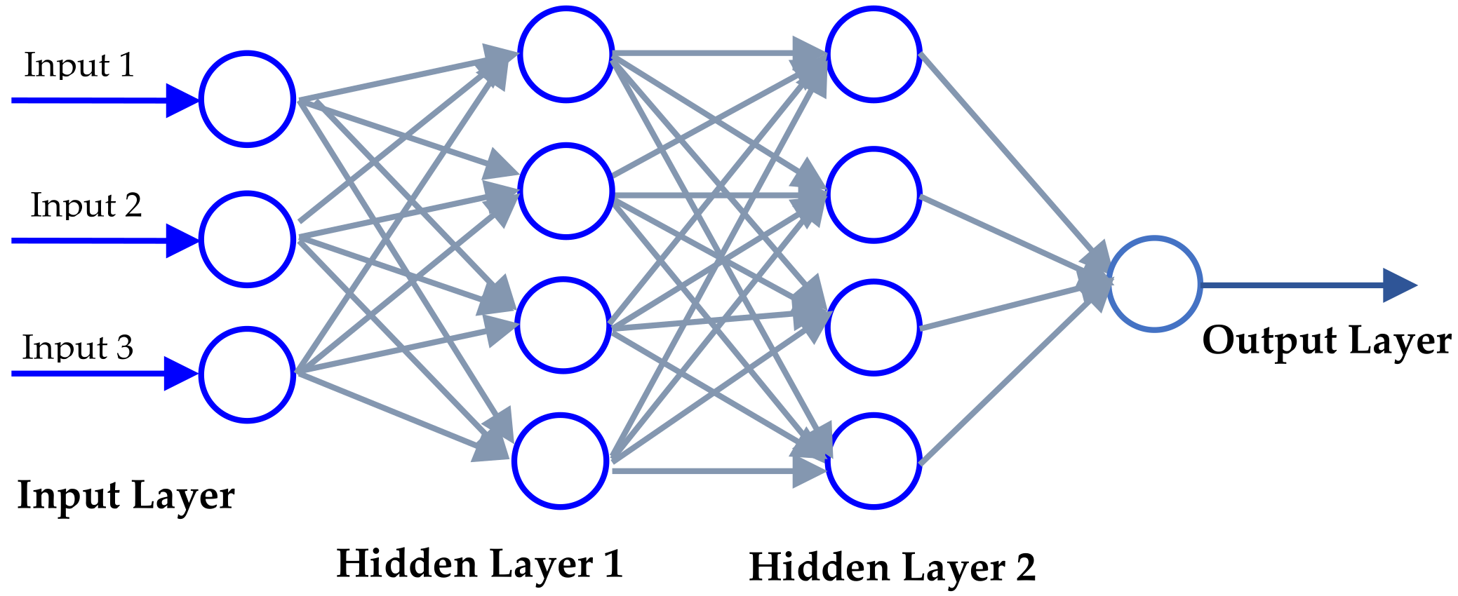
3.5. Proposed Ensemble and Deep Learning Algorithms

AdaBoost: It was discovered by Yoav Freund and Robert Schapire. AdaBoost was the first popular boosting method for binary classification. The Boosting method combines a multiple “weak classifier” into a single “strong classifier” [47].

Bagging: Bagging, also known as Bootstrap aggregation, is a type of ensemble MLT that makes it easier to improve the MLT performance and accuracy. It reduces the error of a prediction model by applying bias-variance trade-offs to an agreement. Bagging is used in regression and classification models to prevent data from being over-fit [48].

Max Voting: The Max Voting method is an MLT which uses a set of ensemble methods and produces the outcomes (class) according to the class with the highest possibility. It basically sums the outcomes from each classifier submitted to a voting classifier and forecasts the result class based on the highest number of votes. Generally, a single model is developed which educates on numerous models and guesses outputs based on the collective number of votes for every output class, instead of building distinct single models and judging their performance [49].

Gradient boosting: The most effective ensemble MLT is the gradient boosting (GB) algorithm. Bias error and variance error are the two most common forms of mistakes in MLTs. The GB algorithm is a boosting method that may be used to reduce the algorithm’s bias inaccuracy. The GB method is employed not just for constant target variables such as regression, but also for categorical target variables such as classifiers. The mean square error (MSE) is the cost function when used as a regression, while the log loss is the cost function when used as a classifier [50].

XGBoost: The XGBoost is also identified as the extreme gradient boosting algorithm. It is a tree-based MLA with better presentation and speediness. XGBoost was created by Tianqi Chen and is controlled mainly by the DMLC (Distributed Machine Learning Community) group. It has gained popularity while yielding desirable results in structured and tabular data.

Artificial neural network (ANN): The ANN, also known as a neural network (NN), is a mathematical model that draws on features of biological neural networks, including their structure and functionality. A neural network uses an artificial neural method of computation to process data and is made up of a network of artificial neurons linked to one another [51]. The ANN has three layers: an input layer, a hidden layer, and an output layer., as shown in Figure 2.

Convolutional neural network (CNN): One of the best-known and most frequently utilized deep learning methods is the convolutional neural network (CNN). CNN’s key benefit over its forerunners is that it recognizes important elements without human intervention, making it popular [53].

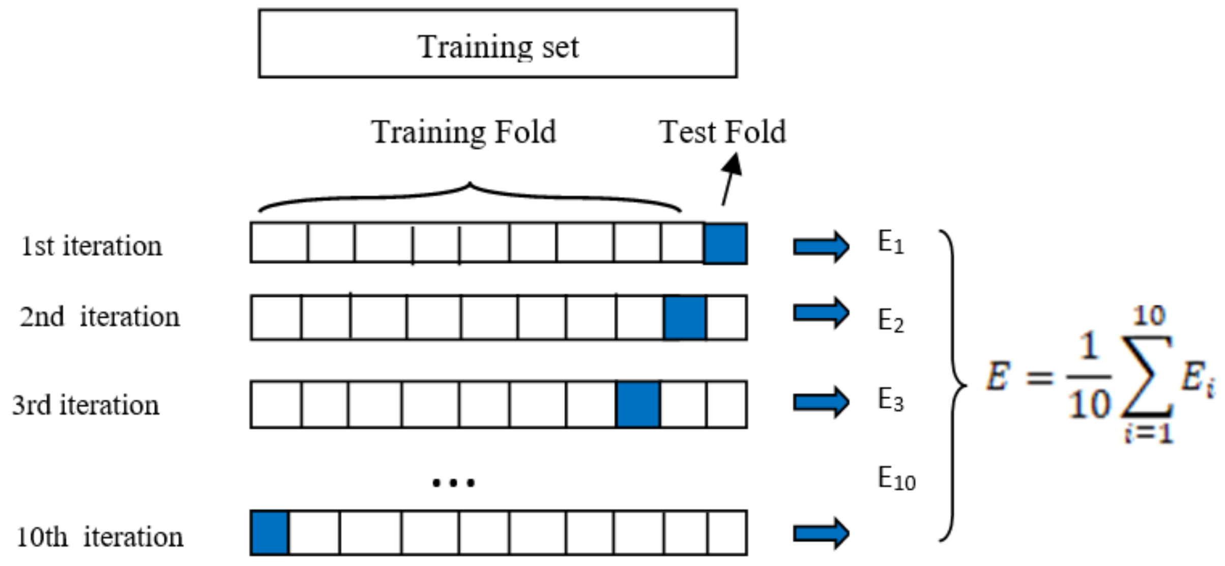
3.6. Evaluation Methodology

As the datasets are small, we used ten-fold cross-validation in order to obtain better model performance. Figure 3 shows all the processes of the ten-fold cross-validation.

3.7. Key Measurements of Performance

In this study, we evaluated the performance of various experiments. The confusion matrix (CM) was calculated. The actual and expected information detected by code smell detection classifiers was stored in the CM. Then using the CM, the true positive (TP), true negative (TN), false positive (FP), and false-negative (FN) were calculated. The definition of TP, TN, FP, and FN are given below:

• TP represents the outputs (occurrences) where the algorithm accurately expects the positive class.
• TN represents the outputs (occurrences) where the algorithm accurately expects the negative class.
• FP represents the outputs (occurrences) where the algorithm inaccurately expects the positive class.
• FN represents the outputs (occurrences) where the algorithm inaccurately expects the negative class.

Definitions and formula of evaluation metrics: PPV, sensitivity, F-measure, AUC_ROC_score, accuracy, MCC, and Cohen_Kappa_score used to evaluate the model’s performance are given below:

Positive predictive value (PPV):Positive predictive value measures the number of code smell instances correctly identified by machine learning methods. PPV is also known as precision [55]. Formula (3) was used to calculate the positive predictive value. PPV is calculated as the number of TP divided by the total number of TP and FP.

$$\mathrm{Positive} \mathrm{Predictive} \mathrm{Value}\left(\mathrm{PPV}\right)=\frac{\mathrm{TP}}{\mathrm{TP}+\mathrm{FP}}$$

(3)

Sensitivity: Sensitivity measures the amount of code smell occurrences recognized by machine learning methods. The sensitivity is also known as the true positive rate (TPR) and Recall [55]. Formula (4) was used to calculate the sensitivity. The sensitivity is calculated as the number of TP divided by the total number of TP and FN.

$$\mathrm{Sensitivity}=\frac{\mathrm{TP}}{\mathrm{TP}+\mathrm{FN}}$$

(4)

F-measure: F-measure measures the harmonic mean of positive predictive value (PPV) and sensitivity, and its stand for a balance between their values [55]. Formula (5) was used to calculate the F-measure.

$$\mathrm{F}-\mathrm{measure}\left(\mathrm{F}\right)=2\times \frac{\mathrm{PPV}\times \mathrm{Sensitivity}}{\mathrm{PPV}+\mathrm{Sensitivity}}$$

(5)

AUC_ROC_Score: The AUC_ROC_score is applied to observe the performance of a classification model based on its rate of correct and incorrect classifications. ROC represents the probability, and AUC calculates the degree of separability [55]. It says how much the model is able to distinguish between classes. An outstanding model puts AUC near one, which notifies that it has a good measure of separation. A bad model will have an AUC near 0, notifying that it has the worst measure of separation. Indeed, it means it returns the result and calculates 0s as 1s and 1s as 0s. When an AUC is 0.5, the model has no class separation ability in the model.

Accuracy: Accuracy measures the association between PPV and sensitivity. It displays the percentage of positive and negative instances that were accurately categorized [55]. Formula (6) was used to calculate accuracy. Accuracy is calculated as the total number of TP and TN divided by the total number of TP, TN, FP, and FN.

$$\mathrm{Accuracy}\left(\mathrm{A}\right)=\frac{\mathrm{TP}+\mathrm{TN}}{\mathrm{TP}+\mathrm{TN}+\mathrm{FP}+\mathrm{FN}}$$

(6)

Matthews Correlation Coefficient (MCC): The Matthews correlation coefficient (MCC) is utilized in MLT to determine the quality of two-class or binary classification. It obtains true and false positives and negatives and is normally considered a balanced calculation that can be utilized if the classes are of significantly different sizes [56]. The formula for calculating the MCC is given in Equation (7).

$$\mathrm{MCC}=\frac{\left(\mathrm{TP}\times \mathrm{TN}\right)-\left(\mathrm{FP}\times \mathrm{FN}\right)}{\sqrt{\left(\mathrm{TP}+\mathrm{FP}\right)\left(\mathrm{TP}+\mathrm{FN}\right)\left(\mathrm{TN}+\mathrm{FP}\right)\left(\mathrm{TN}+\mathrm{FN}\right)}}$$

(7)

Cohen_Kappa_Score: Cohen_Kappais a metric which is utilized to evaluate the agreement between two raters. It can also be utilized to evaluate the performance of a classification model [57]. The formula for calculating the Cohen_Kappa is given in Equation (8).

$$\mathrm{Cohen} \mathrm{Kappa}=\frac{P_0-P_e}{1-P_e}$$

(8)

4. The Outcome of Proposed Algorithms

To answer RQ1, we implemented five ensemble and two deep learning algorithms and found the performance accuracy of each algorithm. Additionally, a Chi-square FSA was applied to select the best metrics from each dataset. The best metrics chosen by the Chi-square FSA are shown in Table 4. All experimental findings of each ensemble and deep learning method are presented in

Table 5. Results of AdaBoost algorithm.

Datasets	PPV (%)	Sensitivity (%)	F-Measure (%)	AUC_ROC_Score (%)	Accuracy (%)	MCC (%)	Cohen_Kappa (%)
DC	98	99	99	84.26	98.80	94.47	94.30
GC	97	97	97	87.97	97.62	91.92	91.89
FE	100	100	100	98.72	100	100	100
LM	100	100	100	98.98	100	100	100

,

Table 6. Results of Bagging algorithm.

Datasets	PPV (%)	Sensitivity (%)	F-Measure (%)	AUC_ROC_Score (%)	Accuracy (%)	MCC (%)	Cohen_Kappa (%)
DC	100	100	100	97.92	98.80	94.42	94.42
GC	100	100	100	98.92	97.62	97.55	97.51
FE	100	100	100	94.20	100	100	100
LM	100	100	100	88.80	99.94	100	100

,

Table 7. Results of Max voting algorithm.

Datasets	PPV (%)	Sensitivity (%)	F-Measure (%)	AUC_ROC_Score (%)	Accuracy (%)	MCC (%)	Cohen_Kappa (%)
DC	100	100	100	94.62	98.81	100	100
GC	98	97	98	85.24	97.62	88.97	88.37
FE	100	100	100	97.67	97.87	94.40	94.25
LM	100	100	100	97.62	97.92	80.95	80.95

,

Table 8. Results of Gradient boosting algorithm.

Datasets	PPV (%)	Sensitivity (%)	F-Measure (%)	AUC_ROC_Score (%)	Accuracy (%)	MCC (%)	Cohen_Kappa (%)
DC	100	100	100	92.40	98.80	94.89	94.89
GC	99	99	99	91.84	97.62	92.66	92.62
FE	100	100	100	97.25	95.74	90.20	89.72
LM	100	100	100	95. 66	100	100	100

,

Table 9. Results of XGboost algorithm.

Datasets	PPV (%)	Sensitivity (%)	F-Measure (%)	AUC_ROC_Score (%)	Accuracy (%)	MCC (%)	Cohen_Kappa (%)
DC	100	100	100	92.54	99.80	100	100
GC	98	99	99	87.26	97.62	94.69	94.54
FE	100	100	100	93.40	100	92.36	92.07
LM	100	100	100	84.33	100	100	100

,

Table 10. Results of ANN algorithm.

Datasets	PPV (%)	Sensitivity (%)	F-Measure (%)	AUC_ROC_Score (%)	Accuracy (%)	MCC (%)	Cohen_Kappa (%)
DC	96	96	96	93.64	97.82	95.52	95.12
GC	96	96	96	92.89	97.23	96.26	96.12
FE	98	98	98	97.28	97.98	99.12	99.08
LM	98	97	98	96.29	98.25	98.78	98.66

and

Table 11. Results of CNN algorithm.

Datasets	PPV (%)	Sensitivity (%)	F-Measure (%)	AUC_ROC_Score (%)	Accuracy (%)	MCC (%)	Cohen_Kappa (%)
DC	98	99	98	93.64	97.82	95.52	95.12
GC	99	99	98	92.89	97.23	96.26	96.12
FE	100	99	100	99.12	99.08	99.12	99.08
LM	100	100	99	99.29	99.26	98.78	98.66

. In each experiment table, we have shown seven performance measurements: PPV, Sensitivity, F-measure, AUC_ROC_score, Accuracy, MCC, and Cohen_Kappa_score. The performance comparison of all five ensemble and two deep learning algorithms is shown in

Table 12. Comparison Performance between Five Ensemble and Two Deep Learning Methods code smells Datasets.

Algorithms	DC			GC			FE			LM
	F (%)	AUC (%)	A (%)	F (%)	AUC (%)	A (%)	F (%)	AUC (%)	A (%)	F (%)	AUC (%)	A (%)
AdaBoost	99.00	84.26	98.80	97.00	87.97	97.62	100	98.72	100	100	98.98	100
Bagging	100	97.92	98.80	100	98.92	97.62	100	94.20	100	100	88.80	99.94
Max voting	100	94.62	98.81	98.00	85.24	97.62	100	97.67	97.87	100	97.62	97.92
Gradient Boosting	100	92.40	98.80	99.00	91.84	97.62	100	97.25	95.74	100	95. 66	100
XGBoost	100	92.54	99.80	99.00	87.26	97.62	100	93.40	100	100	84.33	100
ANN	96.00	93.64	97.82	96.00	92.89	97.23	98.00	97.28	97.98	98.00	96.29	98.25
CNN	98.00	93.64	97.82	98.00	92.89	97.23	100	99.12	99.08	99.00	99.29	99.26

Note: F—F-score, AUC—AUC_ROC_Score, A—Accuracy.

.

4.1. PerformanceComparisonbetweenFive Ensemble and Two Deep Learning Methods

This section compares the outcomes of all five used ensemble and two deep learning techniques applied on ten features selected by the Chi-square FSAs. Table 12 shows comparative performance of all applied ensemble and two deep learning techniques using the AUC ROC Score, F-measure, and Accuracy. From Table 12 it isclear that the AdaBoost approach obtains the highest accuracy of 100% for the FE and LM datasets, while the worst accuracy of 97.62% is for the GC dataset. The Bagging algorithm obtains the highest accuracy of 100% for the FE dataset and the worst accuracy of 97.62% for the GC dataset. The Max voting approach achievedthe best accuracy, 98.81%, for the DC dataset and the worst accuracy, 97.62%, for the GC dataset. The Gradient boosting algorithm obtainedthe highest accuracy of 100% for the LM data set and the worst accuracy of 95.74% for the FE dataset. The XGBoost approach obtainedthe highest accuracy of 100% for the FE and LM datasets, while the worst accuracy was 97.62% for the GC dataset. The ANN approach obtainedthe highest accuracy of 98.25% for the LM datasets, while the worst accuracy was 97.23% for the GC dataset. The CNN approach obtainedthe highest accuracy of 99.26% for the LM datasets, while the worst accuracy was 97.23% for the GC dataset.

4.2. Effect of Subset of Features Selected by Chi-Square FSA on Model Accuracy

Chi-square FSAs were used to answer RQ2. This experiment was done to see the effect of Chi-square FSA to identify the software features which are important in recognizing the code smells.

Table 13. Outcomes of Ensemble algorithms for different sets of selected features.

MLT	Number of Selected Features	Accuracy for DC Dataset (%)	Accuracy for GC Dataset (%)	Accuracy for FE Dataset (%)	Accuracy for LM Dataset (%)
Adaboost algorithm	8	96.43	95.23	100	100
	9	97.61	97.62	100	100
	10	98.80	97.62	100	100
	11	98.80	97.62	97.87	97.91
	12	97.61	97.62	100	100
	All features	98.80	97.62	100	100
Bagging algorithm	8	99.92	98.80	97.87	97.92
	9	97.62	97.62	97.87	97.92
	10	98.80	97.62	100	99.94
	11	97.62	98.80	97.87	100
	12	97.62	99.24	100	100
	All Features	98.80	98.80	97.87	100
Max voting algorithm	8	98.81	95.24	97.87	97.92
	9	100	97.61	97.87	100
	10	98.81	97.62	97.87	97.92
	11	98.80	97.62	100	97.92
	12	98.80	96.42	91.45	97.92
	All Features	97.62	95.23	100	100
Gradient boosting algorithm	8	99.96	98.80	100	100
	9	98.80	96.43	100	100
	10	98.80	97.62	95.74	100
	11	99.28	98.80	95.74	100
	12	98.80	97.62	97.87	100
	All features	98.80	98.80	97.87	100
XGboost algorithm	8	98.80	96.42	97.87	100
	9	98.80	97.62	97.87	100
	10	99.80	97.62	100	100
	11	99.88	98.80	99.56	97.92
	12	99.26	97.62	97.87	97.92
	All features	98.80	97.62	97.87	97.92
ANN	8	97.23	97.12	97.98	97.96
	9	97.23	97.14	97.98	97.96
	10	97.82	97.23	97.98	98.25
	11	98.67	97.98	98.76	98.25
	12	98.62	97.23	98.98	99.02
	All features	99.12	97.56	98.76	98.25
CNN	8	97.82	97.12	98.76	98.88
	9	97.82	97.23	98.98	98.88
	10	97.82	97.23	99.08	99.26
	11	98.98	98.24	99.08	99.26
	12	99.26	98.24	99.56	99.36
	All features	99.16	98.78	99.36	99.26

shows how the performance accuracy of the ensemble and deep learning approaches is affected when the number of selected metrics isincreased by one in each step. The comparison indicates that the feature extraction is helpful to improve the accuracy of nearly all ensemble methods for all datasets, and that it has slightly different effects on each model and each dataset. However, in some models, such as Bagging, Gradient boosting, XGBoost algorithms, ANN, and CNN, the FSA increases accuracy greatly. In Adaboosting and the Max voting algorithm, feature extraction had no significant effect.

4.3. Effect of Class Balancing Technique (SMOTE) on Model Accuracy

A class balancing technique (SMOTE) was used to answer RQ3. This experiment was performed to see the effect of SMOTE on the accuracy performance of code smell detection.

Table 14. Outcomes of Ensemble algorithms with and without applied SMOTE.

Algorithms	DC		GC		FE		LM
	Accuracy with Applied SMOTE	Accuracy without Applied SMOTE	Accuracy with Applied SMOTE	Accuracy without Applied SMOTE	Accuracy with Applied SMOTE	Accuracy without Applied SMOTE	Accuracy with Applied SMOTE	Accuracy without Applied SMOTE
AdaBoost	99.10	98.80	98.21	97.62	98.65	100	100	100
Bagging	99.11	99.92	98.21	99.24	100	100	100	100
Max voting	99.10	100	98.21	97.62	100	100	100	100
Gradient Boosting	100	99.96	99.10	98.80	100	100	100	100
XGBoost	100	99.88	97.32	98.80	98.64	100	100	100
ANN	99.12	98.67	98.37	97.98	99.06	98.98	99.00	99.02
CNN	99.26	99.26	98.78	98.78	99.24	99.56	99.67	99.36

shows how the SMOTE class balancing technique’s performance accuracy affects each ensemble and deep learning method’s performance accuracy for each code smell dataset. The comparison indicates that the SMOTE is helpful in improving the accuracy of some models such asAdaBoost, GB, XGBoost, and ANN models for the DC dataset. Likewise, the AdaBoost, Max voting, GB, and ANN model enhance the accuracy of the GC dataset.

5. Discussion

5.1. Result Comparison of Our Approach with Others’ Correlated Work

A few other authors [22,30,31,33,42] also worked on the same code smell datasets. These authors used machine learning and stack ensemble learning algorithms. In this subsection, we compared the outcomes of our approach with previous related works. They are shown in

Table 15. Result comparison of our approach with other correlated works.

Year	Author Name	Datasets
		DC		GC		FE		LM
		Best Algorithm	Accuracy (%)	Best Algorithm	Accuracy (%)	Best Algorithm	Accuracy (%)	Best Algorithm	Accuracy (%)
2016	Fontana et al. [7]	B-J48 Pruned	99.02	Naive Bayes	97.55	B-JRip	96.64	B-J48 Pruned	99.43
2018	Nucci et al. [36]	RF and J48	Approx 83	J48 and RF	Approx 83	J48 and RF	Approx 84	J48 and RF	Approx 82
2020	Mhawishet al. [25]	RF	99.70	GBT	98.48	Decision tree	97.97	RF	95.97
2020	Guggulothu et al. [20]	-	-	-	-	B-J48 Pruned	99.10	RF	95.90
2021	Alazba et al. [22]	Stack-LR	98.92	Stack-SVM	97.00	Stack-LR	95.38	Stack-SVM	99.24
2021	Dewangan et al. [23]	RF	99.74	RF	98.21	Decision tree	98.60	Logistic Regression	100.00
	Proposed Approach	Max Voting	100	Bagging	99.24	All five methods	100	All Five Methods	100

.

Dewangan et al. [23] achieved 99.74% accuracy with the RF technique employing all features on the DC dataset. Fontana et al.’s [7] approach applied human-understandable detection rules for J48 and JRip algorithms and found 99.02% highest accuracy for the B-J48 Pruned approach. Mhawish et al. [25] used the GA-based FSA and found the highest accuracy, 99.70%, using the RF approach. Nucci et al. [36] applied the gain ratio FSA and found around 83% accuracy with the RF and J48 approach. Alazba et al. [22] used the gain FSA and found the highest accuracy, 98.92%, using the Stack-LR algorithm, whereas this approach’s accuracy was 100% using the Max voting algorithm with nine features.

Dewangan et al. [23] achieved 98.21% accuracy utilizing the RF method with Chi-square FSA on the GC dataset. Fontana et al. [7] applied human-understandable detection rules for the J48 and JRip algorithms and found 97.55% highest accuracy in the Naive Bayes algorithm. Mhawish et al. [25] used the GA-based FSA and found the highest accuracy, 98.48%, using the GBT model. Nucci et al. [36] applied the gain ratio FSA and found around 83% accuracy with the RF and J48 approach. Alazba et al. [22] used the gain FSA and found the highest accuracy, 97%, using the Stack-SVM algorithm, whereas this experiment’s accuracy was 99.24% with the Bagging approach using 12 features.

Dewangan et al. [23] used the Decision tree algorithm with all features and achieved 98.60% accuracy on the FE dataset. Fontana et al.’s [7] approach applied human-understandable detection rules for the J48 and JRip algorithms and found 96.64% greatest accuracy with the B-JRip approach. Mhawish et al. [25] used the GA-based FSA and found the greatest accuracy of 97.97% with the Decision tree approach. Nucci et al. [36] applied the gain ratio FSA, and obtained accuracy of around 84% with the RF and J48 approach. Alazba et al. [22] used the gain FSA and found the greatest accuracy, 95.38%, using the Stack-LR algorithm. Guggulothu et al. [20] converted the dataset into the multi-label dataset, and found the greatest accuracy of 99.10% with the B-J48 Pruned approach. Whereas this approach’s accuracy was100% using all five algorithms (where the AdaBoost model used eight, nine, 10, 12 and all features, the Bagging model used10 and 12 features, the Max voting model used11 and all features, the GB model used eight and nine features, and the XGB model used 10 features).

Dewangan et al. [23] used the Logistic regression approach using all features and achieved 100% accuracy on the LM dataset. Fontana et al.’s [7] approach applied human-understandable detection rules for the J48 and JRip algorithm and found 99.43% greatest accuracy using the B-J48 pruned approach. Mhawish et al. [25] used the GA-based FSA and found the greatest accuracy of 95.97% with the RF approach. Nucci et al. [36] applied the gain ratio FSA and found 82% accuracy with the J48 and RF approaches. Guggulothu et al. [20] converted the dataset into the multi-label dataset, and they found the greatest accuracy of 95.90% with the RF algorithm. Alazba et al. [22] used the gain FSA and found the greatest accuracy, 99.24%, using the Stack-SVM algorithm. Whereas this approach’s accuracy was 100% using all five algorithms (where the AdaBoost model used eight, nine, 10, 12 and all features, the Bagging model used11, 12 and all features, the Max voting model used nine and all features, the GB model used eight, nine, 10, 11, 12, and all features, and the XGB model used eight, nine, and 10 features).

5.2. Analysis of Our Work

In this paper, we have mainly focused on ensemble, deep learning algorithms, the SMOTE balancing technique, and the Chi-square FSA. In this experiment, we established that the ensemble algorithm found the best results compared to our previous work [23], in which six MLTs were applied. We showed our outcomes obtained from five ensemble and two deep learning algorithms in Table 5, Table 6, Table 7, Table 8, Table 9, Table 10 and Table 11. All comparisons of our outcomes with other previous works are shown in Table 15. We used seven performance measurements for evaluating the model’s performance: PPV, Sensitivity, F-measure, AUC_ROC_score, Accuracy, MCC, and Cohen_Kappa_score. All proposed ensemble algorithms produced excellent results for DC, FE, and LM datasets. This research work answers the research questions (discussed in the introduction section).

To answer the RQ1, Five ensemble and two deep learning models are applied. Ensemble approaches have been shown to be quite good at predicting code smells. Furthermore, to answer the RQ2: the Chi-square FSA is applied to improve the performance accuracy. The best metrics are identified by the Chi-square FSA as shown in Table 4. The results indicate that it improves the accuracy of all ensemble methods for all datasets. However, the improvement is different for each model and dataset combination. Bagging, Gradient boosting, and XGBoost algorithms give the best accuracy, but feature extraction has no significant effect on the Max voting algorithm. Our implemented code and datasets are available at the link: https://github.com/seemadewangan/AdaBoost-Model-with-Chi-square-.git(accessed on 4 September 2022). To answer the RQ3, we applied a SMOTE balancing technique.

5.3. Result and All Model Comparison of Our Approach with Other Correlated Works

This subsection presents models applied by various authors and the greatest accuracy they obtained for the same dataset (Data class, God class, Feature envy, and Long method). The previous literature [7,20,22,36,37] proposed various types of machine learning, and ensemble learning algorithms on the same datasets (Fontana et al. [7]), and each author found different results.

Table 16. Result and all model comparison of our approach with other correlated works.

Author Name	Applied Algorithms		Datasets
			DC	GC	FE	LM
		Applied FSA and Other Techniques	Accuracy (%) with Best Algorithm	Accuracy (%) with Best Algorithm	Accuracy (%) with Best Algorithm	Accuracy (%) with Best Algorithm
Fontana et al. [7]	B-J48 Pruned, B-J48 UnPruned, JRip Pruned, JRipUnPruned, RF, Naive Bayes, SMO LibSVM, B-Random Forest, B-JRip, J48 Reduced Error Pruning, B-J48 Reduced Error Pruning	-	99.02% accuracy using B-J48 Pruned	97.55% accuracy using Naive Bayes	96.64% accuracy using B-JRip	99.43% accuracy using B-J48 Pruned
Nucci et al. [36]	B J48 Pruned, B J48 Unpruned, J48 Reduced Error Pruning, B-J48 Reduced Error Pruning, B JRip, B-RF, B-Naive Bayes, B SMO RBF, B SMO Poly, B LibSVM C-SVC Linear, B LibSVM C-SVC Poly, B LibSVM C-SVC Radial, B LibSVM C-SVC Sigmoid, RF, Naive Bayes, SMO RBF, SMO Polynomial, LibSVM C-SVC Linear, LibSVM C-SVC Poly, LibSVM C-SVC Radial, LibSVM C-SVC Sigmoid	GainRatio FSA	Approx 83% accuracy using RF and J48	Approx 83% accuracy using J4 and RF	Approx 84% accuracy using J48 and RF	Approx 82% accuracy using J48 and RF
Mhawishet al. [25]	Deep learning, DT, GBT, SVM, RF, MLP	Genetic Algorithm based FSA and Grid search-based parameter optimization technique	99.70% accuracy using RF	98.48% accuracy using GBT	97.97% accuracy using DT	95.97% accuracy using RF
Guggulothuet al. [20]	J48 Pruned, RF, B-J48 Pruned, B-J48 UnPruned, B-Random Forest	-	-	-	99.10% accuracy using B-J48 Pruned	95.90% accuracy using RF
Alazba et al. [22]	DT, SVM(Lin), SVM(Sig), SVM(Poly), SVM(RBF), NB(B), NB(M), NB(G), LR, MLP, SGD, GP, KNN, LDA, Stack-LR, Stack-DT, Stack-SVM	Gain FSA	98.92% accuracy using Stack-LR	97.00% accuracy using Stack-SVM	95.38% accuracy using Stack-LR	99.24% accuracy using Stack-SVM
Dewangan et al. [23]	Naive Bayes, KNN, DT, MLP, LR, RF	Chi-squared and Wrapper-based FSA, and Grid search parameter optimization	99.74% accuracy using RF	98.21% accuracy using RF	98.60% accuracy using DT	100% accuracy using LR
P.S. Yadav et al. [37]	decision tree model with hyper parameter tuning	Grid search parameter optimization	97.62% accuracy using DT	97.62% accuracy using DT	-	-
Proposed Approach	AdaBoost, Bagging, Max voting, GB, XGBoost, ANN, CNN	Chi-squared FSA, and SMOTE class balancing technique	100% accuracy using Max voting	99.24% accuracy using Bagging	100% accuracy using all five ensemble methods	100% accuracy using all five ensemble methods

shows all the model names applied in the previous literature.

Various authors applied machine learning and ensemble learning algorithms for the data class dataset. First, Fontana et al. [7] created this dataset and applied machine learning to it. They found 99.02% greatest accuracy using the B-J48 Pruned algorithm. After that, Mahvish et al. [25] obtained the greatest accuracy, 99.70%, using the RF model. They applied Deep learning and five other machine learning algorithms with genetic algorithm-based FSA and Grid search-based parameter optimization techniques. Dewangan et al. [23] also applied six machine learning algorithms with the Chi-square and Wrapper-based FSA and Grid search parameter optimization and obtained 99.74% greatest accuracy using RF. But in the earlier literature, the authors neither handled class imbalance nor studied the performance of boosting and bagging ensemble learning algorithms. Therefore, in this work, we applied five ensemble learning and two deep learning algorithms with the Chi-square FSA and SMOTE class balancing techniques. We obtained 100% accuracy using the Max voting algorithm. In this way, we found that ensemble learning is the best algorithm for detecting the code smells from the data class dataset.

For the god class dataset, first, Fontana et al. [7] created this dataset and applied sixteen machine learning models to these. They found 97.55% greatest accuracy using the Naïve Bayes algorithm. After that, Mahvish et al. [25] obtained the greatest accuracy, 98.48%, using the GBT model. They applied Deep learning and five other machine learning algorithms with genetic algorithm-based FSA and Grid search-based parameter optimization techniques. Dewangan et al. [23] also applied six machine learning algorithms with Chi-square, Wrapper-based FSA and Grid search parameter optimization and obtained 98.21% greatest accuracy using the RF, which is not a good result as compared to previous literature. But in the earlier literature, the authors neither handled class imbalance nor studied the performance of boosting and bagging ensemble learning algorithms. Therefore, in this work, we applied five ensemble learning, two deep learning algorithms with Chi-square FSA and the SMOTE class balancing technique. We obtained 99.24% accuracy using the Bagging algorithm. In this way, we found that ensemble learning is the best algorithm for detecting the code smells from the god class dataset.

Various authors applied machine learning and ensemble learning algorithms for the feature envy dataset. First, Fontana et al. [7] created this dataset and applied machine learning to it. They found 96.64% greatest accuracy using the B-JRip algorithm. After that, Mahvish et al. [25] obtained the greatest accuracy, 97.97%, using the DT model. They applied Deep learning and five other machine learning algorithms with the genetic algorithm-based FSA and Grid search-based parameter optimization techniques. Guggulothu et al. [20] applied five machine learning algorithms and obtained 99.10%, the greatest accuracy using the B-J48 Pruned algorithm. Dewangan et al. [23] also applied six machine learning algorithms with Chi-square and Wrapper-based FSA and Grid search parameter optimization and obtained 98.60% greatest accuracy using the DT model, which is not a good result as compared to previous literature. But in the earlier literature, the authors neither handled class imbalance nor studied the performance of boosting and bagging ensemble learning algorithms. Therefore, in this work, we applied five ensemble learning, two deep learning algorithms with Chi-square FSA, and the SMOTE class balancing technique. We obtained 100% accuracy using all five ensemble models (AdaBoost, Bagging, Max voting, GB, XGBoost). In this way, we found that ensemble learning is the best algorithm for detecting the code smells from the feature envy dataset.

For the Long method dataset also, various authors applied various types of machine learning and ensemble learning algorithms. First, Fontana et al. [7] created this dataset and applied machine learning to it. They found 99.43% greatest accuracy using the B-J48 Pruned algorithm. After that, Alazba et al. [22] obtained the greatest accuracy of 99.24% using the Stack-SVM model. They applied 17machine learning algorithms with the gain FSA. Dewangan et al. [23] also applied six machine learning algorithms with Chi-square and Wrapper-based FSA and Grid search parameter optimization and obtained 100% greatest accuracy using the LR. But in the earlier literature, the authors neither handled class imbalance nor studied the performance of boosting and bagging ensemble learning algorithms. Therefore, in this work, we applied five ensemble learning and two deep learning algorithms with the Chi-square FSA, and the SMOTE class balancing technique. We obtained 100% accuracy using all five ensemble models (AdaBoost, Bagging, Max voting, GB, XGBoost). In this way, we found that ensemble learning is the best algorithm for detecting the code smells from the feature envy dataset.

5.4. Statistical Analysis

We used a Paired t-test to find out whether there was a statistically significant difference between the two classifiers such that we could employ only the best one. This paired t-test needs the utilization of N different test sets on which to calculate each classifier. We used ten-fold cross-validation for N test sets. The accuracy for each classifier across each code smell dataset is shown in

Table 17. Statistical Analysis.

Classifier	Data Class (%)	God Class (%)	Feature Envy (%)	Long Method (%)
AdaBoost	98	97	97	97
Bagging	80	90	80	90
Max voting	97	98	98	99
Gradient Boosting	98	97	97	97
XGBoost	97	97	98	97
ANN	80	90	80	90
CNN	80	90	80	90

. We calculated the statistical analysis with ten-fold cross-validation through the F-measure using a Paired t-test. We observed that for the Data class dataset, the GradientBoosting and AdaBoost algorithms were the highest-scoring algorithms. For the God class dataset, the Max voting algorithm was the highest-scoring algorithm. For the feature envy dataset, the Maxvoting and XGBoost algorithms were the highest-scoring algorithms. For the Long method dataset, the Maxvoting algorithm was the highest-scoring algorithm. Therefore, the Maxvoting classifier is best for code smell detection.

5.5. Threats to Validity

This subsection discusses threats related to internal validity, external validity, and conclusion validity. One of the threats to internal validity is the dataset. It is the most serious internal threat to our experiment. As mentioned above, Fontana et al. [7] developed the dataset that we used for this study. They created the database by employing code smells consultants to choose candidates from a large collection of 74 diverse software applications (Qualitas Corpus) and carefully certifying the 420 instances to every code smell. To create this collection of datasets, many metrics (features) are assessed. Many of these metrics may or may not have an effect on the outcomes of the models that were applied. The second threat to internal validity is the feature selection technique that we used- Chi-square FSAs. Chi-Square is sensitive to small frequencies in features considered. Generally, when the expected value in a feature is less than five, the Chi-square can lead to errors in conclusions. To handle this threat, we analyzed the datasets and found that this condition does not occur in our dataset.

Threats to external validity in our study are as follows: The first issue is that the dataset only contains two code smells: class-level and method-level smells. The second vulnerability is connected to the software applications that are used to produce the dataset, which are entirely in Java language code. As a result, our technique may not be suitable for C and C++ programming languages.

Threats to conclusion validity are summarized as follows: They are related to evaluating the model’s performance. The metrics we used for evaluation of models’ performance may not suffice. We tried to manage this threat by using multiple evaluation metrics, such as PPV, Sensitivity, F-measure, AUC_ROC_score, Accuracy, MCC, and Cohen_Kappa_score. It was further improved using ten-fold cross-validation.

6. Conclusions and Future Scope

This paper proposed ensemble and deep learning methods to detect the code smells. Four code smell datasets, DC, GC, FE, and LM, were used, created by Fontana et al. [7], using 74 open-source systems. The Chi-square FSA was applied to select the best metrics from each dataset to improve performance accuracy.

The five ensemble MLTs (AdaBoost, Bagging, Max Voting, Gradient Boosting, XGBoost), and two deep learning (ANN and CNN) are applied to detect the code smells. This research work is implemented two-fold: (i) the first fold applied ensemble approaches to detect the code smells and (ii) the seven performance measurements (PPV, Sensitivity, F-measure, AUC_ROC_score, Accuracy, MCC, and Cohen_Kappa_score) are computed in the second fold to compare these ensemble MLTs. Chi-square FSAs with a ten-fold cross-validation approach wereused to improve accuracy.

The AdaBoost algorithm achieved the greatest accuracy of 100% for the FE and the LM datasets when the number of selected features were eight, nine, 10, and 12, and the whole set of metrics, while the worst accuracy was 95.23% for the GC dataset when the number of selected features was eight.

The Bagging algorithm achieved the greatest accuracy of 100% for the FE (when the number of selected features were 10and 12) and the LM (when the number of selected features were 11, 12and the whole set of metrics) datasets. The worst accuracy of 97.62% was achieved for the DC (when the number of selected features were nine, 11, and 12) and GC (when the number of selected features were nine and 10) datasets.

The Max Voting algorithm obtained the greatest accuracy of 100% for the DC (when the number of selected features was nine), the FE (when the number of selected features was11, and the whole set of metrics), and the LM (when the number of selected features wasnine and the whole set of metrics) datasets. The worst accuracy, 91.45%, was obtained for the FE dataset for 12 selected features.

The Gradient Boosting algorithm obtained the greatest accuracy of 100% for the FE (when the number of selected features was eight and nine) and the LM (when the number of selected features was eight, nine, 10, 11, 12 and the whole set of metrics) datasets, while the worst accuracy, 95.74%, was obtained for the FE dataset if the number of selected features was 10 and 11.

The XGBoost algorithm obtains the greatest accuracy of 100% for, the FE (when the number of selected features was 10) and the LM (when the number of selected features was eight, nine, and 10) datasets, while the worst accuracy of 96.42% was obtained for GC if the number of selected features was eight.

The ANN algorithm obtains the greatest accuracy of 99.12% for the DC (when all features were selected), while the worst accuracy of 97.12% was obtained for the GC if the number of selected features was eight.

The CNN algorithm obtains the highest accuracy of 99.56% for the FE (when the number of selected features was 12), while the worst accuracy of 97.12% was obtained for the GC if the number of selected features was eight.

We utilized two kinds of smells in this paper: class and method level smell with limited features. This paper presents several experiments that would be interesting for software developers as well as research practitioners working in this or a similar domain.

In future work, we are planning to improve results by applying algorithms to solve data augmentation techniques. Other learning algorithms as well as feature selection techniques should also be explored to find the best techniques for code smell detection.

References

1. Palomba, F.; Bavota, G.; Penta, M.D.; Oliveto, R.; Poshyvanyk, D.; de Lucia, A. Mining Version Histories for Detecting Code Smells. IEEE Trans. Softw. Eng. 2015, 41, 4062–4089. [Google Scholar] [CrossRef]
2. Wikipedia Contributors. Code Smell. 20 October 2021. Available online: https://en.wikipedia.org/w/index.php?title=Code_smell&oldid=1050826229 (accessed on 16 November 2021).
3. Kessentini, W.; Kessentini, M.; Sahraoui, H.; Bechikh, S.; Ouni, A. A cooperative parallel search-based software engineering approach for code-smells detection. IEEE Trans. Softw. Eng. 2014, 40, 841–861. [Google Scholar] [CrossRef]
4. Fontana, F.A.; Braione, P.; Zanoni, M. Automatic detection of bad smells in code: An experimental assessment. J. Object Technol. 2012, 11, 5. [Google Scholar]
5. Dewangan, S.; Rao, R.S. Code Smell Detection Using Classification Approaches. In Intelligent Systems; Udgata, S.K., Sethi, S., Gao, X.Z., Eds.; Lecture Notes in Networks and Systems; Springer: Singapore, 2022; Volume 431. [Google Scholar] [CrossRef]
6. Rasool, G.; Arshad, Z. A review of code smell mining techniques. J. Softw. Evol. Process 2015, 27, 867–895. [Google Scholar] [CrossRef]
7. Fontana, F.A.; Mäntylä, M.V.; Zanoni, M.; Marino, A. Comparing and experimenting machine learning techniques for code smell detection. Empir. Softw. Eng. 2016, 21, 1143–1191. [Google Scholar] [CrossRef]
8. Lehman, M.M. Programs, life cycles, and laws of software evolution. Proc. IEEE 1980, 68, 1060–1076. [Google Scholar] [CrossRef]
9. Wiegers, K. , Beatty, J. Software Requirements; Pearson Education: London, UK, 2013. [Google Scholar]
10. Chung, L.; do Prado Leite, J.C.S. On Non-Functional Requirements in Software Engineering. In Conceptual Modeling: Foundations and Applications-Essays in Honor of John Mylopoulos; Borgida, A.T., Chaudhri, V., Giorgini, P., Yu, E., Eds.; Springer: Singapore, 2009; pp. 363–379. [Google Scholar]
11. Fowler, M.; Beck, K.; Brant, J.; Opdyke, W.; Roberts, D. Refactoring: Improving the Design of Existing Code, 1st ed.; Addison-Wesley Professional: Boston, MA, USA, 1999. [Google Scholar]
12. Yamashita, A.; Moonen, L. Do Code Smells Reflect Important Maintainability aspects? In Proceedings of the 28th IEEE International Conference Software Maintenance, Trento, Italy, 23 September 2012; pp. 306–315. [Google Scholar]
13. Sjøberg, D.I.K.; Yamashita, A.; Anda, B.C.D.; Mockus, A.; Dyb, A.T. Quantifying the effect of code smells on maintenance effort. IEEE Trans. Softw. Eng. 2013, 39, 1144–1156. [Google Scholar] [CrossRef]
14. Sahin, D.; Kessentini, M.; Bechikh, S.; Ded, K. Code-smells detection as a bi-level problem. ACM Trans. Softw. Eng. Methodol. 2014, 24, 6. [Google Scholar] [CrossRef]
15. Olbrich, S.M.; Cruzes, D.S.; Sjoøberg, D.I.K. Are all Code Smells Harmful? A study of God Classes and Brain Classes in the evolution of Three open-Source Systems. In Proceedings of the 26th IEEE International Conference Software Maintenance, Timisoara, Romania, 12–18 September 2010. [Google Scholar]
16. Khomh, F.; Penta, D.M.; Gueheneuc, Y.G. An Exploratory Study of the Impact of Code Smells on Software Change Proneness. In Proceedings of the 16th Working Conference on Reverse Engineering, Lille, France, 13–16 October 2009; pp. 75–84. [Google Scholar]
17. Deligiannis, I.; Stamelos, I.; Angelis, L.; Roumeliotis, M.; Shepperd, M. A controlled experiment investigation of an object-oriented design heuristic for maintainability. J. Syst. Softw. 2004, 72, 129–143. [Google Scholar] [CrossRef]
18. Li, W.; Shatnawi, R. An empirical study of the bad smells and class error probability in the post-release object-oriented system evolution. J. Syst. Softw. 2007, 80, 1120–1128. [Google Scholar] [CrossRef]
19. Perez-Castillo, R.; Piattini, M. Analyzing the harmful effect of god class refactoring on power consumption. IEEE Softw. 2014, 31, 48–54. [Google Scholar] [CrossRef]
20. Guggulothu, T.; Moiz, S.A. Code smell detection using multi-label classification approach. Softw. Qual. J. 2020, 28, 1063–1086. [Google Scholar] [CrossRef] [Green Version]
21. Lewowski, T.; Madeyski, L. How far are we from reproducible research on code smell detection? A systematic literature review. Inf. Softw. Technol. 2022, 144, 106783. [Google Scholar] [CrossRef]
22. Alazba, A.; Aljamaan, H.I. Code smell detection using feature selection and stacking ensemble: An empirical investigation. Inf. Softw. Technol. 2021, 138, 106648. [Google Scholar] [CrossRef]
23. Dewangan, S.; Rao, R.S.; Mishra, A.; Gupta, M. A Novel Approach for Code Smell Detection: An Empirical Study. IEEE Access 2021, 9, 162869–162883. [Google Scholar] [CrossRef]
24. Sharma, T.; Efstathiou, V.; Louridas, P.; Spinellis, D. Code smell detection by deep direct-learning and transfer-learning. J. Syst. Softw. 2021, 176, 110936. [Google Scholar] [CrossRef]
25. Mhawish, M.Y.; Gupta, M. Predicting code smells and analysis of predictions: Using machine learning techniques and software metrics. J. Comput. Sci. Technol. 2020, 35, 1428–1445. [Google Scholar] [CrossRef]
26. Mhawish, M.Y.; Gupta, M. Generating Code-Smell Prediction Rules Using Decision Tree Algorithm and Software Metrics. Int. J. Comput. Sci. Eng. 2019, 7, 41–48. [Google Scholar] [CrossRef]
27. Pushpalatha, M.N.; Mrunalini, M. Predicting the Severity of Closed Source Bug Reports Using Ensemble Methods. In Smart Intelligent Computing and Applications. Smart Innovation, Systems and Technologies; Satapathy, S., Bhateja, V., Das, S., Eds.; Springer: Singapore, 2019; Volume 105. [Google Scholar] [CrossRef]
28. Pandey, S.K.; Tripathi, A.K. An Empirical Study towards dealing with Noise and Class Imbalance issues in Software Defect Prediction. Soft Comput. 2021, 25, 13465–13492. [Google Scholar] [CrossRef]
29. Boutaib, S.; Bechikh, S.; Palomba, F.; Elarbi, M.; Makhlouf, M.; Said, L.B. Code smell detection and identification in imbalanced environments. Expert Syst. Appl. 2021, 166, 114076. [Google Scholar] [CrossRef]
30. Fontana, F.A.; Zanoni, M. Code smell severity classification using machine learning techniques. Knowl. Based Syst. 2017, 128, 43–58. [Google Scholar] [CrossRef]
31. Baarah, A.; Aloqaily, A.; Salah, Z.; Mannam, Z.; Sallam, M. Machine Learning Approaches for Predicting the Severity Level of Software Bug Reports in Closed Source Projects. Int. J. Adv. Comput. Sci. Appl. 2019, 10, 285–294. [Google Scholar] [CrossRef] [Green Version]
32. Pushpalatha, M.N.; Mrunalini, M. Predicting the severity of open source bug reports using unsupervised and supervised techniques. Int. J. Open Source Softw. Process. 2019, 10, 676–692. [Google Scholar] [CrossRef]
33. Kaur, I.; Kaur, A. A Novel Four-Way Approach Designed with Ensemble Feature Selection for Code Smell Detection. IEEE Access 2021, 9, 8695–8707. [Google Scholar] [CrossRef]
34. Draz, M.M.; Farhan, M.S.; Abdulkader, S.N.; Gafar, M.G. Code smell detection using whale optimization algorithm. Comput. Mater. Contin. 2021, 68, 1919–1935. [Google Scholar] [CrossRef]
35. Gupta, H.; Kulkarni, T.G.; Kumar, L.; Neti, L.B.M.; Krishna, A. An Empirical Study on Predictability of Software Code Smell Using Deep Learning Models; Springer: Cham, Switzerland, 2021. [Google Scholar] [CrossRef]
36. Di Nucci, D.; Palomba, F.; Tamburri, D.A.; Serebrenik, A.; de Lucia, A. Detecting Code Smells using Machine Learning Techniques: Are We There Yet? In Proceedings of the 2018 IEEE 25th International Conference on Software Analysis, Evolution and Reengineering (SANER), Campobasso, Italy, 20–23 March 2018. [CrossRef] [Green Version]
37. Yadav, P.S.; Dewangan, S.; Rao, R.S. Extraction of Prediction Rules of Code Smell using Decision Tree Algorithm. In Proceedings of the 2021 10th International Conference on Internet of Everything, Microwave Engineering, Communication and Networks (IEMECON), Jaipur, India, 1–2 December 2021; pp. 1–5. [Google Scholar] [CrossRef]
38. Pecorelli, F.; Palomba, F.; di Nucci, D.; de Lucia, A. Comparing Heuristic and Machine Learning Approaches for Metric-Based Code Smell Detection. In Proceedings of the 2019 IEEE/ACM 27th International Conference on Program Comprehension (ICPC), Montreal, QC, Canada, 25–26 May 2019; pp. 93–104. [Google Scholar] [CrossRef]
39. Alkharabsheh, K.; Crespo, Y.; Manso, E.; Taboada, J.A. Software Design Smell Detection: A systematic mapping study. Softw. Qual. J. 2019, 27, 1069–1148. [Google Scholar] [CrossRef]
40. Alkharabsheh, K.; Crespo, Y.; Fernández-Delgado, M.; Viqueira, J.R.; Taboada, A.J. Exploratory study of the impact of project domain and size category on the detection of the God class design smell. Softw. Qual. J. 2021, 29, 197–237. [Google Scholar] [CrossRef]
41. Mansoor, U.; Kessentini, M.; Maxim, B.R.; Deb, K. Multi-objective code-smells detection using good and bad design examples. Softw. Qual. J. 2017, 25, 529–552. [Google Scholar] [CrossRef]
42. Tempero, E.; Anslow, C.; Dietrich, J.; Han, T.; Li, J.; Lumpe, M.; Melton, H.; Noble, J. The Qualitas Corpus: A Curated Collection of Java Code for Empirical Studies. In Proceedings of the 17th Asia Pacific Software Engenering Conference, Sydney, Australia, 30 November–3 December 2010; pp. 336–345. [Google Scholar]
43. Marinescu, C.; Marinescu, R.; Mihancea, P.; Ratiu, D.; Wettel, R. iPlasma: An Integrated Platform for Quality Assessment of Object-Oriented Design. In Proceedings of the 21st IEEE International Conference on Software Maintenance (ICSM 2005), Budapest, Hungary, 29 September 2005; pp. 77–80. [Google Scholar]
44. Nongpong, K. Integrating “Code Smells” Detection with Refactoring Tool Support. Ph.D. Thesis, University of Wisconsin Milwaukee, Milwaukee, WI, USA, 2012. [Google Scholar]
45. Marinescu, R. Measurement and Quality in Object-Oriented Design. Ph.D. Thesis, Department of Computer Science, “Polytechnic” University of Timisoara, Timisoara, Romania, 2002. [Google Scholar]
46. Peshawa, J.; Muhammad, A.; Rezhna, H.F. Data Normalization and Standardization: A Technical Report. Mach. Learn. Tech. Rep. 2014, 1, 1–6. [Google Scholar]
47. Boosting in Machine Learning | Boosting and AdaBoost. Available online: https://www.geeksforgeeks.org/boosting-in-machine-learning-boosting-and-adaboost/ (accessed on 26 November 2021).
48. Bagging in Machine Learning: Step to Perform and Its Advantages. Available online: https://www.simplilearn.com/tutorials/machine-learning-tutorial/bagging-in-machine-learning#what_is_bagging_in_machine_learning (accessed on 26 November 2021).
49. ML | Voting Classifier using Sklearn. Available online: https://www.geeksforgeeks.org/ml-voting-classifier-using-sklearn/ (accessed on 26 November 2021).
50. How the Gradient Boosting Algorithm Works? Available online: https://www.analyticsvidhya.com/blog/2021/04/how-the-gradient-boosting-algorithm-works/ (accessed on 26 November 2021).
51. Grossi, E.; Buscema, M. Introduction to artificial neural networks. Eur. J. Gastroenterol. Hepatol. 2007, 19, 1046–1054. [Google Scholar] [CrossRef]
52. upGrad. Neural Network: Architecture, Components & Top Algorithms. Available online: https://www.upgrad.com/blog/neural-network-architecture-components-algorithms/ (accessed on 4 September 2022).
53. Alzubaidi, L.; Zhang, J.; Humaidi, A.J.; Al-Dujaili, A.; Duan, Y.; Al-Shamma, O.; Santamaría, J.; Fadhel, M.A.; Al-Amidie, M.; Farhan, L. Review of deep learning: Concepts, CNN architectures, challenges, applications, future directions. J. Big Data 2021, 8, 53. [Google Scholar] [CrossRef]
54. K-Fold Cross-Validation. Available online: http://karlrosaen.com/ml/learning-log/2016-06-20/ (accessed on 4 September 2022).
55. Machine Learning with Python. Available online: https://www.tutorialspoint.com/machine_learning_with_python/machine_learning_algorithms_performance_metrics.html (accessed on 4 September 2022).
56. Phi Coefficient. Available online: https://en.wikipedia.org/wiki/Phi_coefficient (accessed on 4 September 2022).
57. Cohen’s Kappa. Available online: https://en.wikipedia.org/wiki/Cohen%27s_kappa (accessed on 4 September 2022).
Figure 1. Proposed research scheme.
Applsci 12 10321 g001
Figure 2. Artificial neural network [52].
Applsci 12 10321 g002
Figure 3. 10-fold Cross-validation technique [54].
Applsci 12 10321 g003