Simplified Energy Model and Multi-Objective Energy Consumption Optimization of a Residential House

Featured Application

The potential application of the proposed model is a computationally inexpensive semi- or fully automated system for the optimization of operation in residential buildings in terms of energy consumption.

Abstract

Some analyses state that buildings contribute to overall energy consumption by 20–40%, which, in the context of the recent geopolitical energy crisis, makes them a critical issue to study. Finding solutions for better energy management in buildings can have a significant impact on the energy sector, thus reducing EU energy dependencies and contributing to the fulfillment of the REPowerEU goals. This paper focuses on proposing a simplified model of a residential house considering the main appliances, heating and cooling, a photovoltaic system, and electric vehicle recharging. Weather and solar irradiance forecasts are taken into account. The model predicts the energy demands of a house based on online weather forecasts and the desired indoor temperature. The article also focuses on the analysis of how weather forecast uncertainty affects energy demand prediction. This model can be used to better understand and predict the energy demand of either a single house or a set of houses. A multi-objective optimization approach that takes into account the preferences of users/inhabitants is developed to provide a compromise between the price paid for the electricity and temperature comfort. The authors plan to apply the proposed model to a residential house’s real-time control system. The model will be tuned, its predictions will be tested, and it will be used for energy demand optimization.

1. Introduction

The current geopolitical and energy market situations push to further accelerate the EU energy transition to renewable resources, and support Europe’s energy independence from external suppliers and fossil fuels. REPowerEU is the EU Commission’s action plan aiming at making Europe independent from external fossil fuels, in light of the current geopolitical crisis, which is exploiting the large energy dependence of the EU on external countries. The REPowerEU action plan devises a set of measures to steeply reduce dependence on Russian fossil fuels and proceed toward a green transition while growing the resilience of the EU-wide energy system. One of the pillars of the action plan is energy saving.

Buildings account for 20–40% of the overall energy consumption in developed countries, out of which 50% corresponds to heating ventilation air-conditioning (HVAC) systems energy consumption as stated in [1,2]. As the penetration of renewable energy sources rises, the demands on the power grid are growing as the stabilization of the grid becomes more difficult by incorporating these resources [3,4]. Electric vehicles will also become a bigger part of the grid, which will lead to overall higher energy demands as well as greater peaks of this demand during the daytime [5]. However, their storage potential is also large, which might also be used for grid stabilization [6].

A better control strategy can be based on the scheduling of home appliances or more effective renewable energy usage together with energy storage and battery management [7,8,9,10,11].

People need to be accounted for in the models, not only because the models need information about the occupancy in buildings, but mainly because people have their preferences, for example with regard to thermal comfort.

Most articles mention the unreliability of models and predictions. Several articles focus on model predictive control (MPC) [1,3,4,12,13,14] that takes into account the comfort of the residents as well as different types of constraints or uncertainty of predictions. An overview of different state-of-the-art MPC approaches used in buildings, together with weather forecasts and an energy storage system, can be found in [15]. For example, the authors mention different operating strategies of the controller: “demand shaving, demand shifting, energy consumption minimizing, energy cost minimizing, maximal use of renewable energies, etc.”.

Some articles focus on the possibilities of optimization [9,11,15,16,17,18,19], predictions of energy demands/consumption or weather and solar forecasts [11,13,15,20], or the building model where the dynamics are mostly caused due to the heating and cooling systems [9,13,14,15,17,18,19,21,22,23,24,25,26].

Demand response programs can then be used to obtain better control of the energy demands as needed, so as to retain the energy grid stability. There are many articles that focus on the demand response initiative, for example [10,11,27,28]. Demand response methods are mainly used from the perspective of aggregators, to shave the peaks of energy demand. The energy demands of industrial customers seem to be more predictable than that of residential customers [29], but studies that are mentioned above focus on individual consumers. Demand response initiatives will need a well-working infrastructure of control systems in individual buildings. Two-way communication will take into account not just the appliances in the building, but also the preferences of the residents.

Most of the above-mentioned methods and approaches require an energy model of the house. In practice, there are three different approaches to model design, which are models based on physical principles (white box), models based on experimental data (black box) and models using a combination of physics and data (grey box). Buildings are complex non-linear systems that are influenced not only by weather conditions but also by the operating modes and schedules of users. Buildings are usually not equipped with enough sensors and energy metering. The goal is to develop models that are applicable to the online control and optimization of building operations. Modeling also depends on the time scale for which the model is to be used, ranging from short-term modeling for daily operation and planning, to medium-term predictions for system maintenance, to long-term predictions and planning. White-box models use physical laws and relationships and are able to capture the dynamics of the system, but they are time-consuming to build, identify, and solve. Software modeling tools include building energy simulation programs such as EnergyPlus [30], building performance simulation programs such as ESP-r [31], more general simulation tools such as Transient System Simulation Tool (TRNSYS) [32], or open access standards and open-source software such as cyber–physical systems, one of which is Modelica [33]. Models tend to be very complicated, so some authors try to simplify (reduce the order) or linearize the models. Additionally, the creation of such models is quite demanding in terms of expertise and time. The counterpart to these efforts is the use of black-box models that are based only on data. For example, researchers attempt to create models describing the correlation between operational data and energy consumption using multiple linear regression and self-regression methods or neural networks. Hybrid grey-box models use simplified physics to reduce model building, training data, and computational complexity. The authors followed a similar path to, for example, that of [34,35], where a resistance and capacitance network (RC) was proposed to model and predict building cooling load. The authors tried to preserve the physical essence of the original processes, but they reduced the complexity of the description to a minimal model structure with a small number of parameters. The authors plan to use the proposed model in the control system of a residential house with restricted memory and computational power. The model will be used for strategic control but also as part of an expert system allowing the user to make informed decisions. The main electrical appliances are heating (electric), cooling (air conditioning), and charging an electric car. All other appliances have lower power consumption and, as with the charging of the electric car, they are considered to run in the simulation according to a parameterized schedule. The indoor temperature is affected not only by heating and cooling but also by the outside temperature and solar irradiation. Electricity is taken from the grid, and part of it is generated from solar panels. Redundant electricity can overflow back into the grid. It will be possible to continuously evaluate the error of the model and refine certain model descriptions or parameters based on this information.

The authors analyzed the uncertainty of weather forecasts, which translates into the uncertainty of energy consumption prediction and, therefore, the price paid for energy, although this uncertainty was calculated based on the actual forecasted temperature value. Similar work on forecast uncertainties can be found in [28].

The last aim of this work was to propose a multi-objective optimization approach for indoor desired temperature modifications, where the user of such a system receives information about predicted prices for paid electricity based on the weather forecast horizon. This approach allows the user to make an informed decision (trade-off) about thermal comfort and the predicted price paid.

2. Materials and Methods

2.1. Mathematical Model

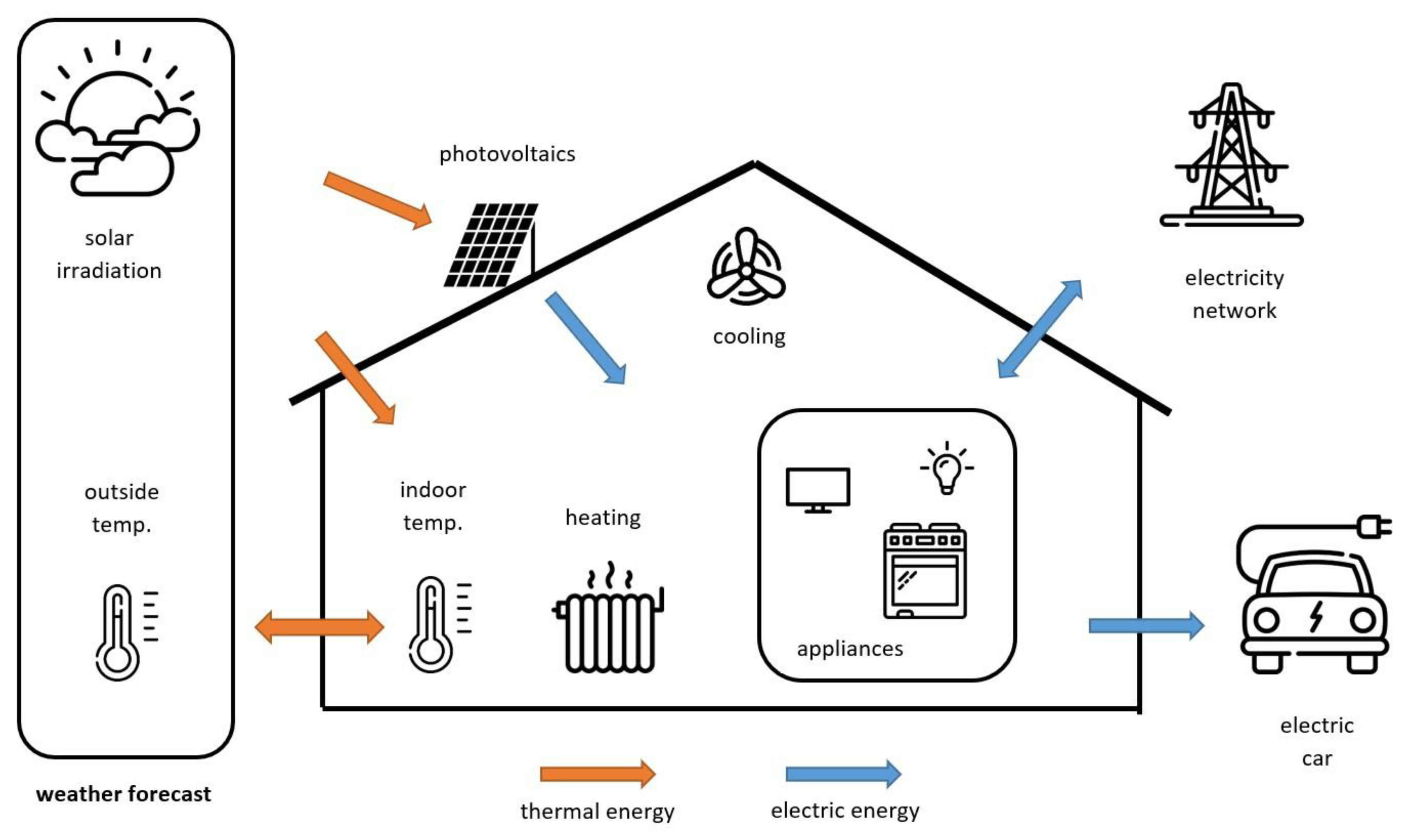
A grey-box energy model of a residential house was created. The model contains several energy sources and appliances—see Figure 1. Firstly, the model contains appliances that have a fixed power consumption when turned on. Although these appliances might not necessarily have a fixed consumption on start-up, such dynamics were not included in the simulation, as the timescale of the simulations was several days. These appliances were built into the model by specifying a timeframe for when they should operate on any given day of the week. Examples of such appliances are kitchen appliances, a washing machine, a TV, a PC, and lighting fixtures.

Secondly, the model contains electric heating and cooling systems that most affect the overall power consumption. Predominantly, the outside temperature and the heating effect of solar irradiation forecasts have the biggest effect on indoor temperature. The heating system respects the demands of the user by keeping the desired temperature.

Thirdly, the model contains a photovoltaic system. Its expected energy generation forecast profile is taken from the average values of solar irradiation in the last several years [36]. The weather forecast also contains information about expected cloudiness. This expected cloudiness was then used to bring variability to the forecasted solar irradiation. Lastly, a model of a battery of an electric vehicle was built into the model but it was only used as an appliance in the current version of the model.

The model was primarily designed for a mid-latitude residential house in Europe, where the most important appliance is heating in winter and cooling in summer. However, it can easily be parameterized for other regions.

2.1.1. Appliances with Constant Power Consumption

Such appliances in the model are kitchen appliances, a washing machine, a TV, a PC, and lighting. All of these are considered to have constant power consumption, so they are defined by their timing during the week.

2.1.2. Sunshine Irradiation Forecast

For the irradiation forecast, a system from the European Union Science Hub called PVGIS (Photovoltaic Geographical Information System) was used [36]. It contains historical data on irradiation in different areas around the world measured for several years. The monthly irradiation data show a typical day’s irradiation of a given month for a given place. In this case, Palermo (Italy) was chosen as the city of interest. Such an irradiation profile was then recalculated based on the expected cloudiness in the upcoming days by:

I_cloud = 0.1 ∙ I_forecasted + 0.9 ∙ (1 − C/100) ∙ I_forecasted,

(1)

where

I_cloud is the irradiation with cloudiness taken into account, W/m²;

I_forecasted is the typical irradiation on a clear day, W/m²;

C is the level of cloudiness, %.

Forecasted irradiation was calculated for each timestep (5 min) using linear interpolation for both the cloudiness forecast and the typical day’s irradiation course.

The attenuation of the irradiation by clouds is considered to be 90%. That means that even when the expected cloudiness level is 100% there is still some part of the irradiation that gets to the surface of the Earth.

The main idea behind the use of (1) was to obtain an approximation of variation in the irradiation on the forecast horizon and to see how such variation would affect the model’s output.

2.1.3. Heating and Cooling Subsystem

Both heating and cooling are connected to the weather forecast. The model takes into account the desired temperature indoors and the forecasted data. The inside temperature is considered to change dynamically. Such dynamics are defined by a constant mass M, which describes heat accumulation. The energy balance is described by the discrete-time differential equation of the simplified zone thermal model [37,38]:

P_heating(k − 1) + P_Sun(k − 1) − P_cooling(k − 1) = K ∙ (T_inside(k − 1) − T_outside(k − 1)) + M ∙ (T_inside(k) − T_inside(k − 1))/T_s,

(2)

where

k is the current time step;

P_heating is the heating power, W;

P_Sun is the heating power of the Sun, W;

P_cooling is the cooling power, W;

K is the thermal loss coefficient, W/°C;

T_outside is the outside temperature, °C;

T_inside is the inside temperature, °C;

M is a constant that consists of mass and specific heat;

T_s is the sampling period, s.

Constants M and K were chosen to reflect experience in a real house; Moreover, the thermal loss coefficient K would change as a function of solar radiation, and convection due to wind speed and conduction.

The simplified zone thermal model provides a simple way for modeling the house (especially in the case of simulation of a large aggregate of buildings) for which more detailed and complicated models cannot be used for real-time optimization. However, more complex methods such as ASHRAE [39] would be more suitable, for example, for comfort evaluations and for the sizing of the HVAC system in the presence of more thermal zones. There are also software programs, such as TRNSYS, that provide the possibility to have detailed simulations. However, the main idea behind this paper was to consider the parts of the model that might affect the resulting energy demands the most.

In order to achieve the desired temperature inside the home, a PI controller was implemented into the model. It was considered that a controller would be present in the building so that the effects of changing the desired temperature could be seen. The PI controller used in the model is described by:

u(k) = u(k-1) + k_P ∙ (1 + T_s/T_i) ∙ e(k) – k_p ∙ e(k-1),

(3)

where

u is the control output for heating or cooling, W;

k is the current timestep;

k_p is the proportional gain of the controller;

T_s is the sampling period, s;

T_i is the integration time constant, s;

e is the control error, °C.

The controller’s output u is calculated in each timestep, defined by the sampling period, from the control error e, which is the difference between the desired indoor temperature and the actual indoor temperature. The control error used in the PI controller is formulated as:

e(k) = w_T(k) – T_inside(k),

(4)

where

w_T is the desired indoor temperature, °C;

T_inside is the measured indoor temperature, °C.

The calculated control output is then used as the heating or cooling power needed for the current time step in order to follow the desired indoor temperature in the next time step. Both heating and cooling have a defined maximal power consumption and efficiency of transforming electrical energy into heating or cooling power, so the control output cannot be infinite but is bounded.

In the first step of the simulation, the actual indoor temperature is considered to be equal to the desired temperature unless the heating or cooling maximal power is exceeded. The amount of heating or cooling power needed to achieve the desired temperature is calculated from the static equation considering the outside temperature and the sunshine power:

u(1) = K ∙ (T_inside(1) − T_outside(1)) − P_Sun(1),

(5)

In case the calculated power exceeds the limits of heating and cooling, then the actual indoor temperature is calculated from the static equation by the following formula, which is taken from Equation (5):

T_inside(1) = (u(1) + P_Sun(1))/K + T_outside(1).

(6)

Then, the desired temperature in the first step is considered to be the same as the calculated indoor temperature in order to start the simulation with a control deviation equal to zero. In the following time steps, the indoor temperature is calculated by:

T_inside(k) = [(P_heating(k − 1) + P_Sun(k − 1) − P_cooling(k − 1) + K ∙ (T_inside(k − 1) − T_outside(k − 1))] ∙ T_s/M + T_inside(k − 1).

(7)

The actual heating and cooling power used for indoor temperature calculation is divided by the efficiency value. Each system has its own efficiency, and its range is between 0 and 1, where 0 means 0% efficiency and 1 means 100% efficiency.

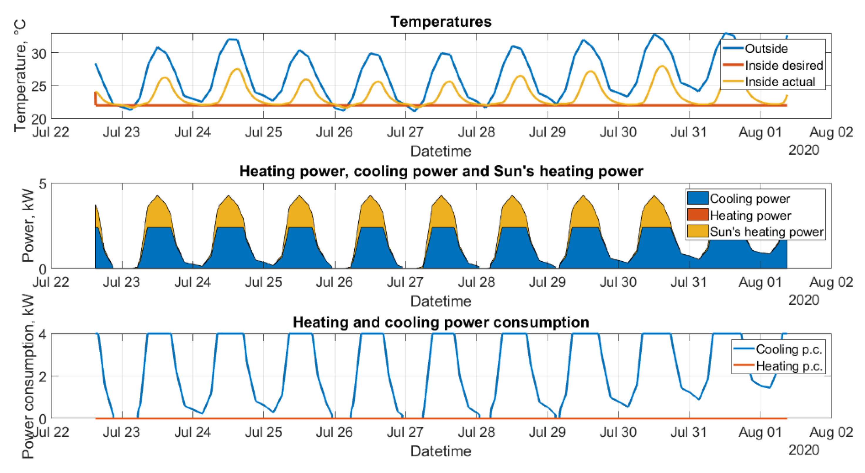
The resulting forecast, shown in Figure 2, was obtained for the building’s thermal loss coefficient of 0.25 kW/°C, M representing mass and specific heat of 3000, heating maximal power consumption of 3 kW with heating efficiency 90%, maximal power consumption of cooling of 4 kW and the efficiency of cooling 60%. These values were chosen based on experience in terms of the energy consumption values of a real house.

The sampling period and the simulation timestep were set to 300 s. The controller’s proportional gain k_P was set to 4 and the parameter of the integration time constant T_i was set to 12,000 s.

The gain of the controller corresponds to the inverse of the system gain, and the integration time constant of the controller is consistent with the dominant time constant of the system. This setting leads approximately to aperiodic control response.

The heating power of sunshine is defined by the area affected by the sun during the day and the solar irradiation forecast by the formula:

P_Sun = I_cloud ∙ A_exposed ∙ k_{solar_heat},

(8)

where

P_Sun is the heating power from the Sun that is transferred indoors, W;

A_exposed is the area that is exposed to the Sun, m²;

k_{solar_heat} is the coefficient of transformation of the irradiation to heating power.

2.1.4. Photovoltaic Subsystem

The photovoltaic subsystem is built into the model in a similar way to the heating power of the sun. It is described by the area of the photovoltaic panels, the irradiation forecast with cloudiness levels, and the efficiency of turning the solar power into electrical power. Electrical power obtained from the photovoltaic panels is described by:

P_pv = I_cloud ∙ A_pv ∙ k_{pv_efficiency},

(9)

where

P_pv is the electrical power generated by the photovoltaics, W;

A_pv is the area of the photovoltaic panels, m²;

k_{pv_efficiency} is the efficiency factor of photovoltaic panels.

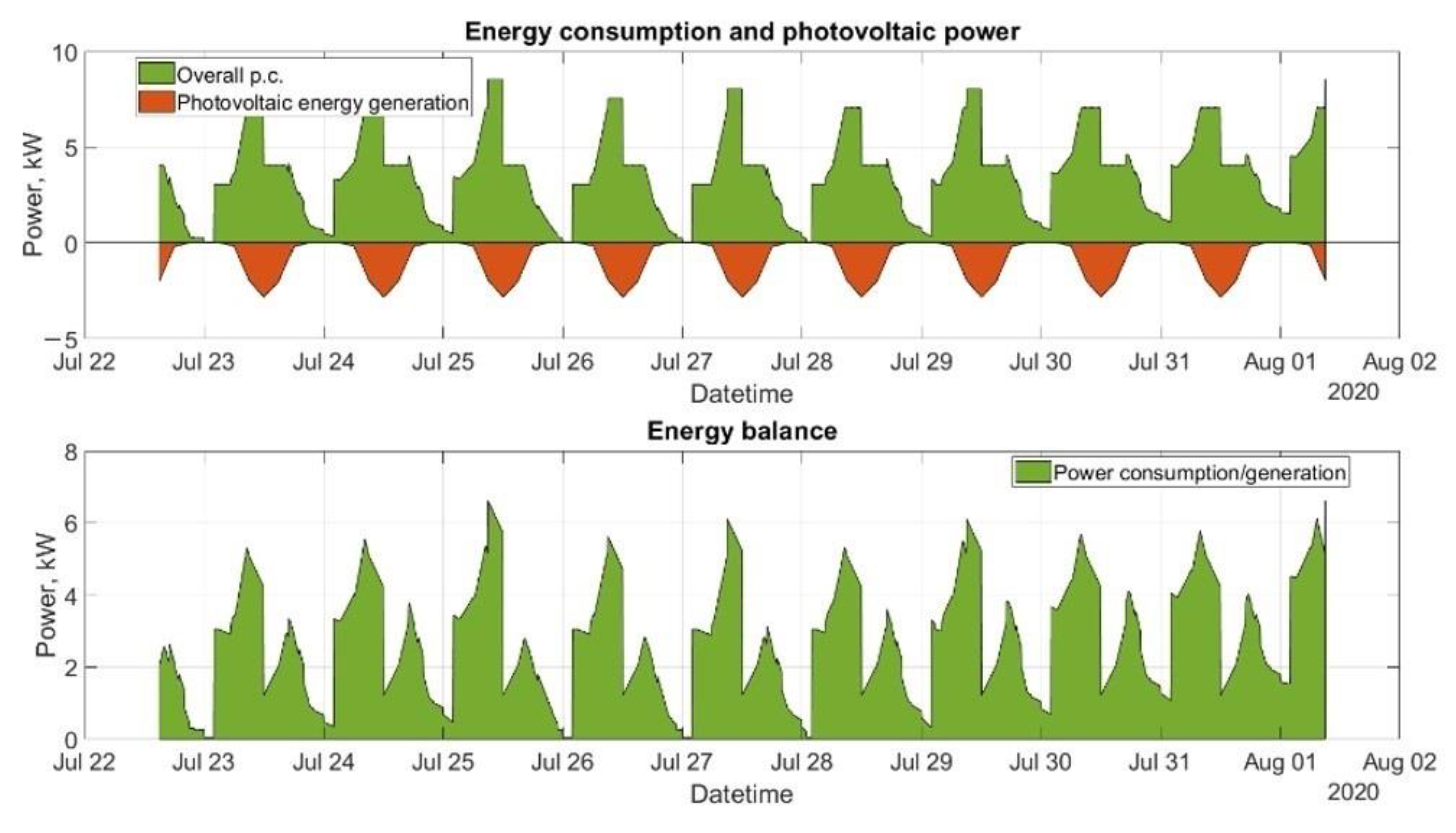
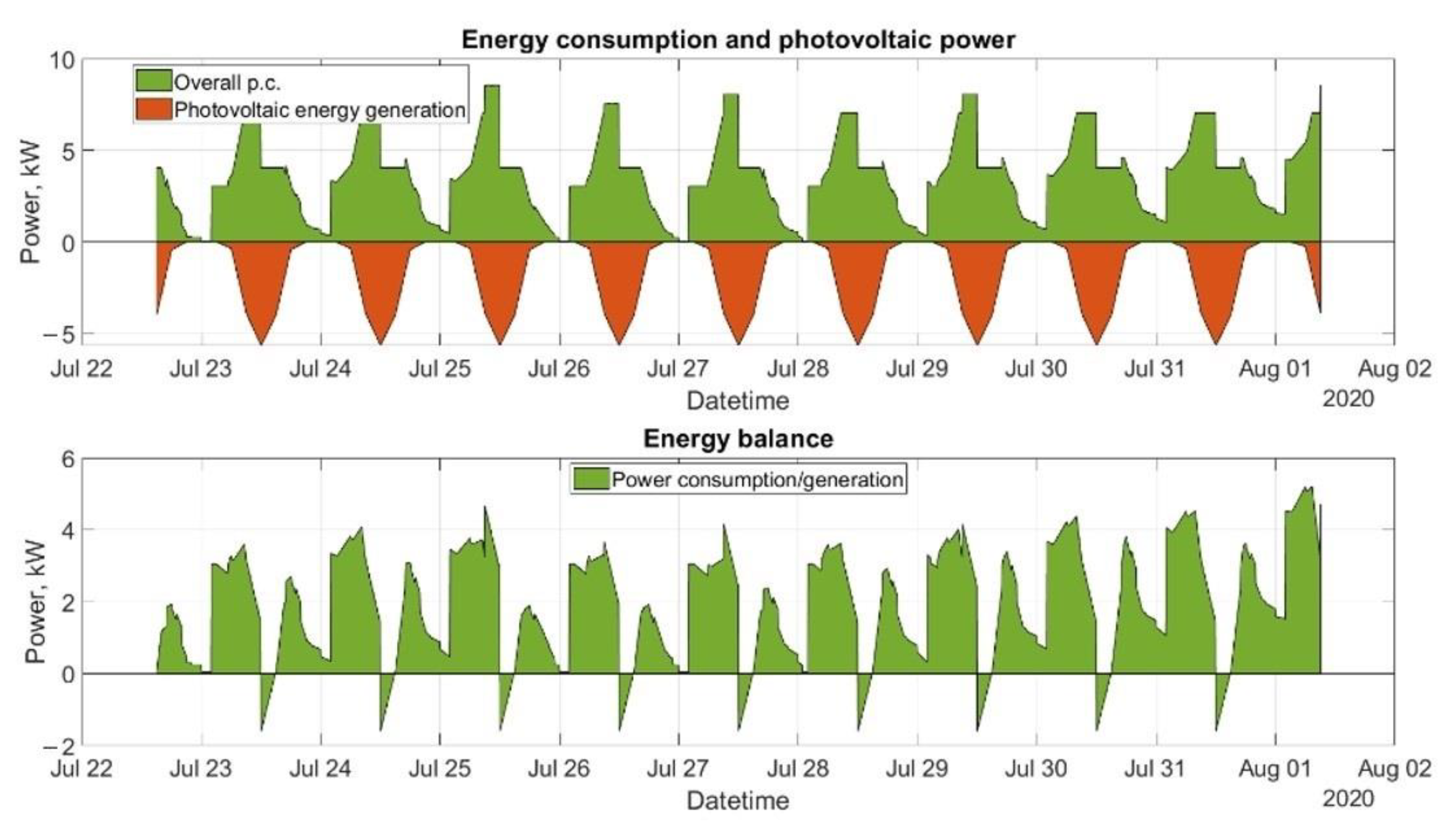
The first part of Figure 3 and Figure 4 shows the overall predicted power consumption of the home and the predicted power generation from the photovoltaic panels. By combining both terms, the overall power consumption of the home is lowered by the power generated by the photovoltaic panels, as shown by the energy balance on the second graph. The surplus of generated energy results in the possibility of selling it back to the grid. These results were obtained for two different areas covered by photovoltaic panels-namely 10 m² and 30 m².

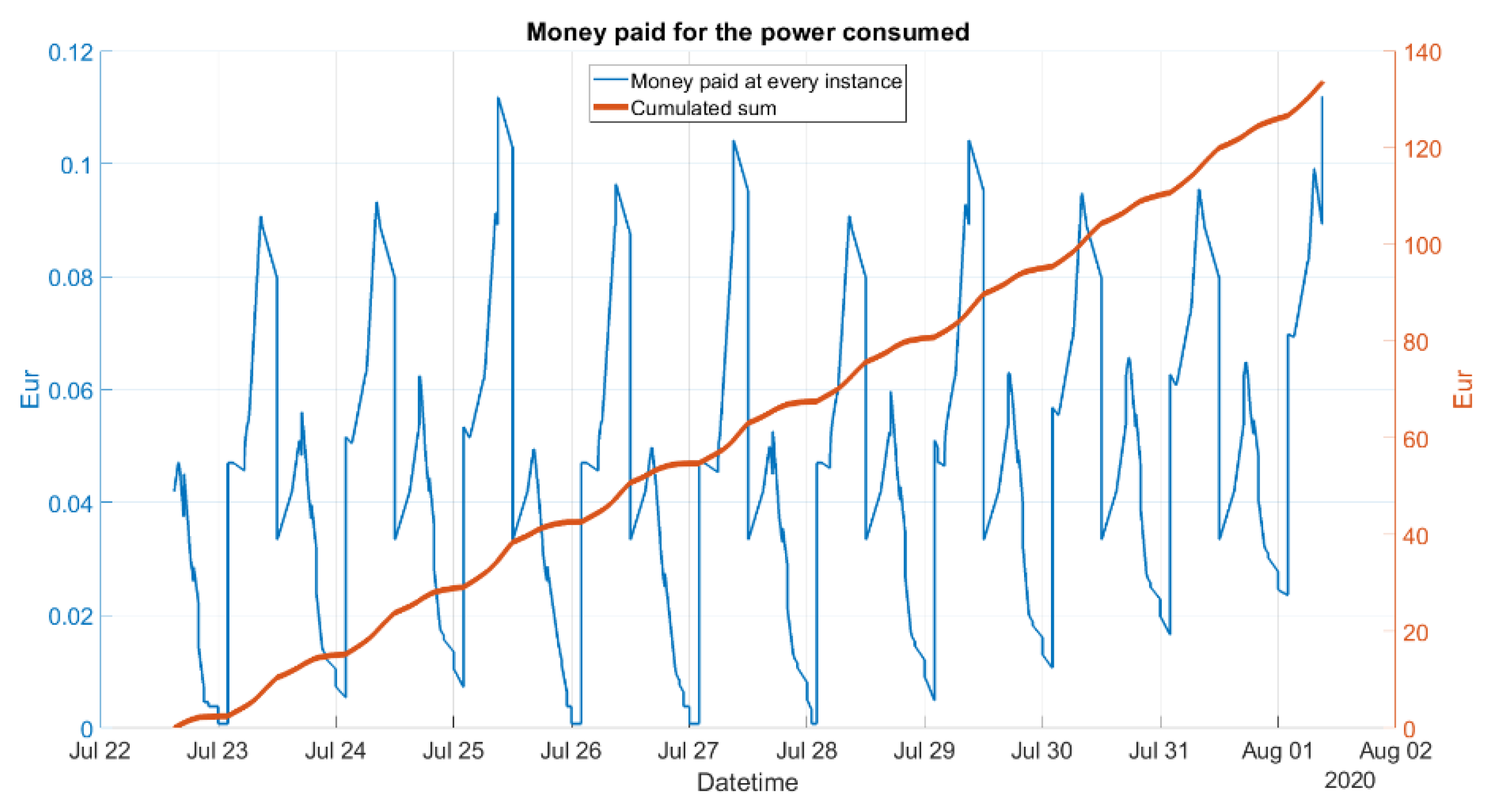
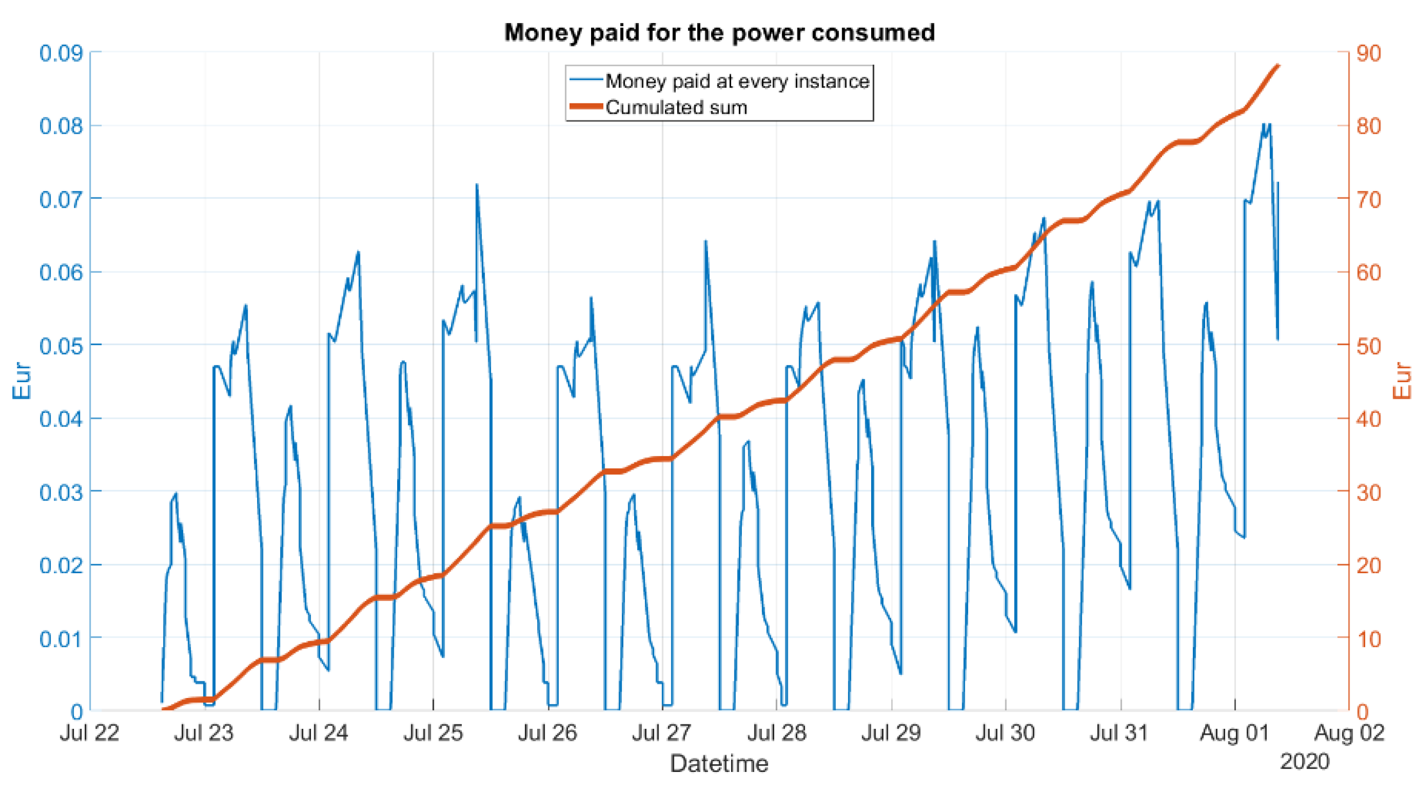
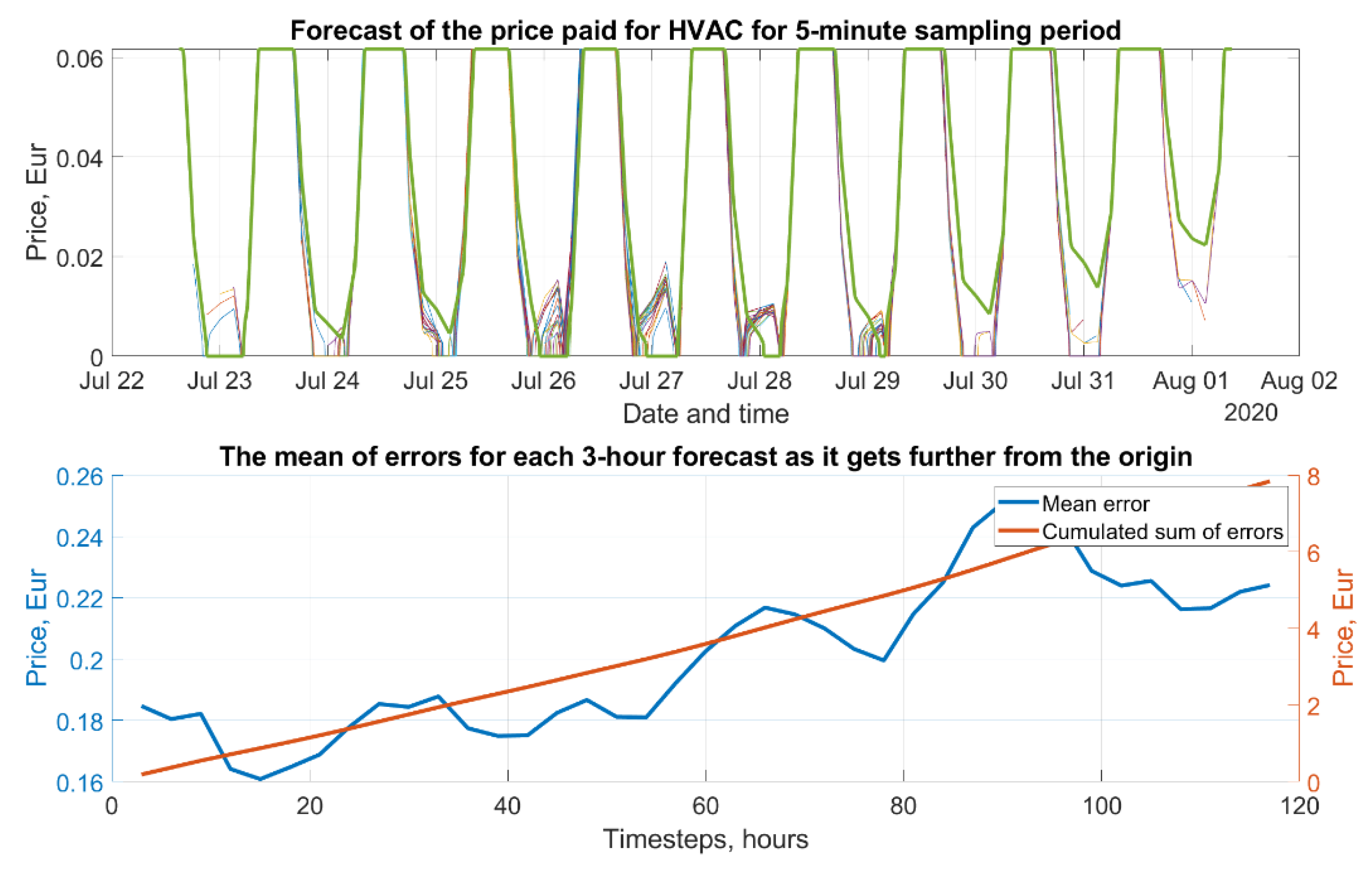
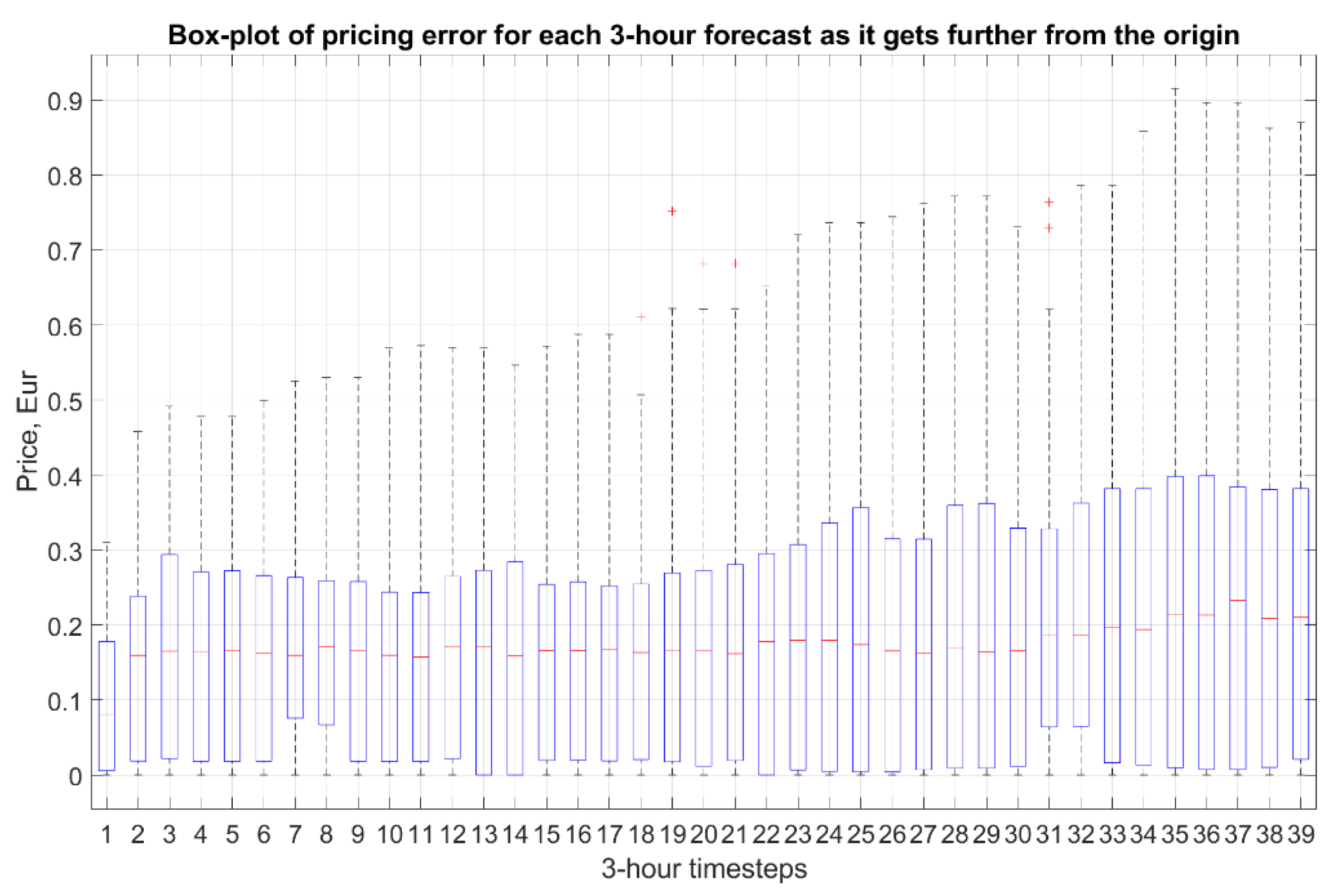
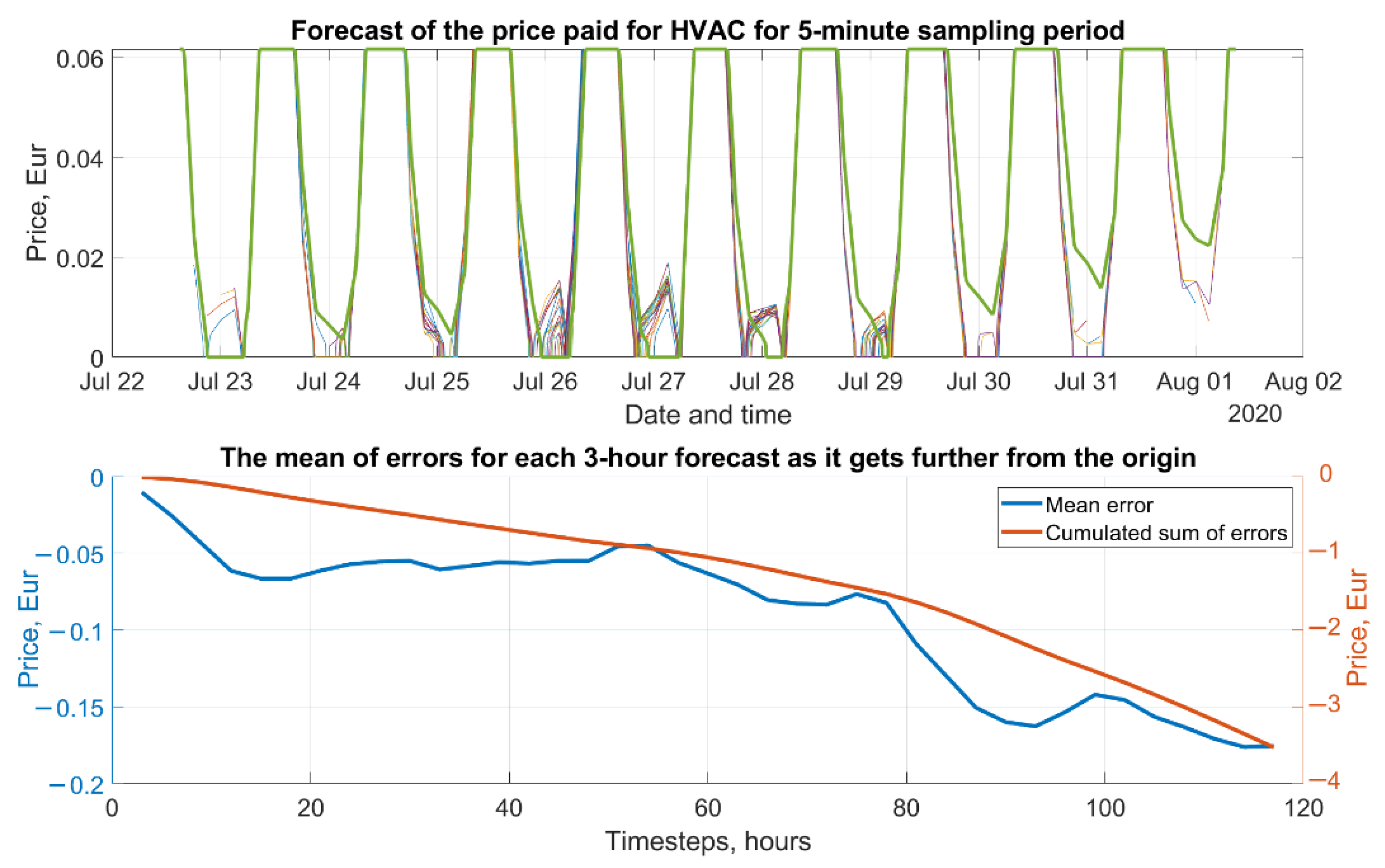
Figure 5 and Figure 6 show the amount of money that is forecasted to be paid in each step as well as a cumulated sum of the money that will be paid on the forecast horizon.

The efficiency of the panels was considered to be constantly 20%. The pricing was considered to be 0.185 EUR per kWh consumed from the grid and 0.018 EUR per kWh sold back to the grid. The tariffs were considered to be fix-priced; however, in future studies, it will be important to consider flexible price tariffs.

2.1.5. Electric Vehicle (EV) Battery Subsystem

The EV battery subsystem in this model is considered only as an appliance. The state of charge (SOC) of the battery in charging mode is given by:

SOC(k) = SOC(k − 1) + P_charging ∙ ε_ch/C_max ∙ 100,

(10)

where

SOC(k) is the state of charge in the current step, %;

SOC(k − 1) is the state of charge in the previous step, %;

P_charging is the charging power, kW;

ε_ch is the charging efficiency;

C_max is the maximum possible battery capacity, kWh.

The discharging mode is described by:

SOC(k) = SOC(k − 1) − P_discharged/ε_d/C_max ∙ 100,

(11)

where

P_discharged is the discharged power on the output of the battery, kW;

ε_d is the discharging efficiency.

The energy from the battery in the model is only used for driving the electric vehicle and not as a supporting energy system for the home, which could be the next feature implemented in the model.

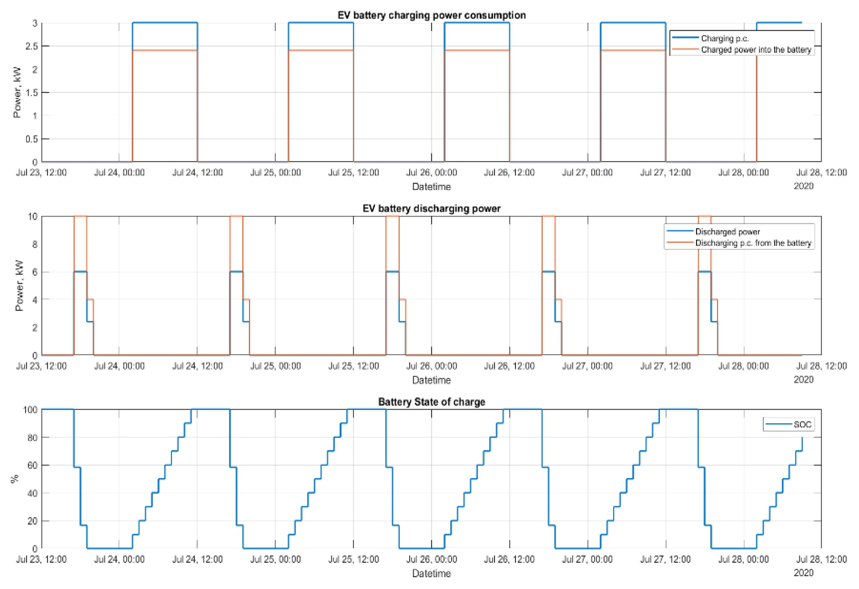
The first part of Figure 7 shows the charging cycles that were fixed in the week. The second part shows the discharging, which reflects the car being driven. These timings were fixed for testing purposes. The third part shows the State of charge of the battery on the forecast horizon.

These results were obtained for the battery defined with a maximum capacity of 24 kWh, maximal charging power of 3 kW, charging efficiency of 80%, maximal discharging power of 6 kW and discharging efficiency of 60%.

2.1.6. Weather Forecast

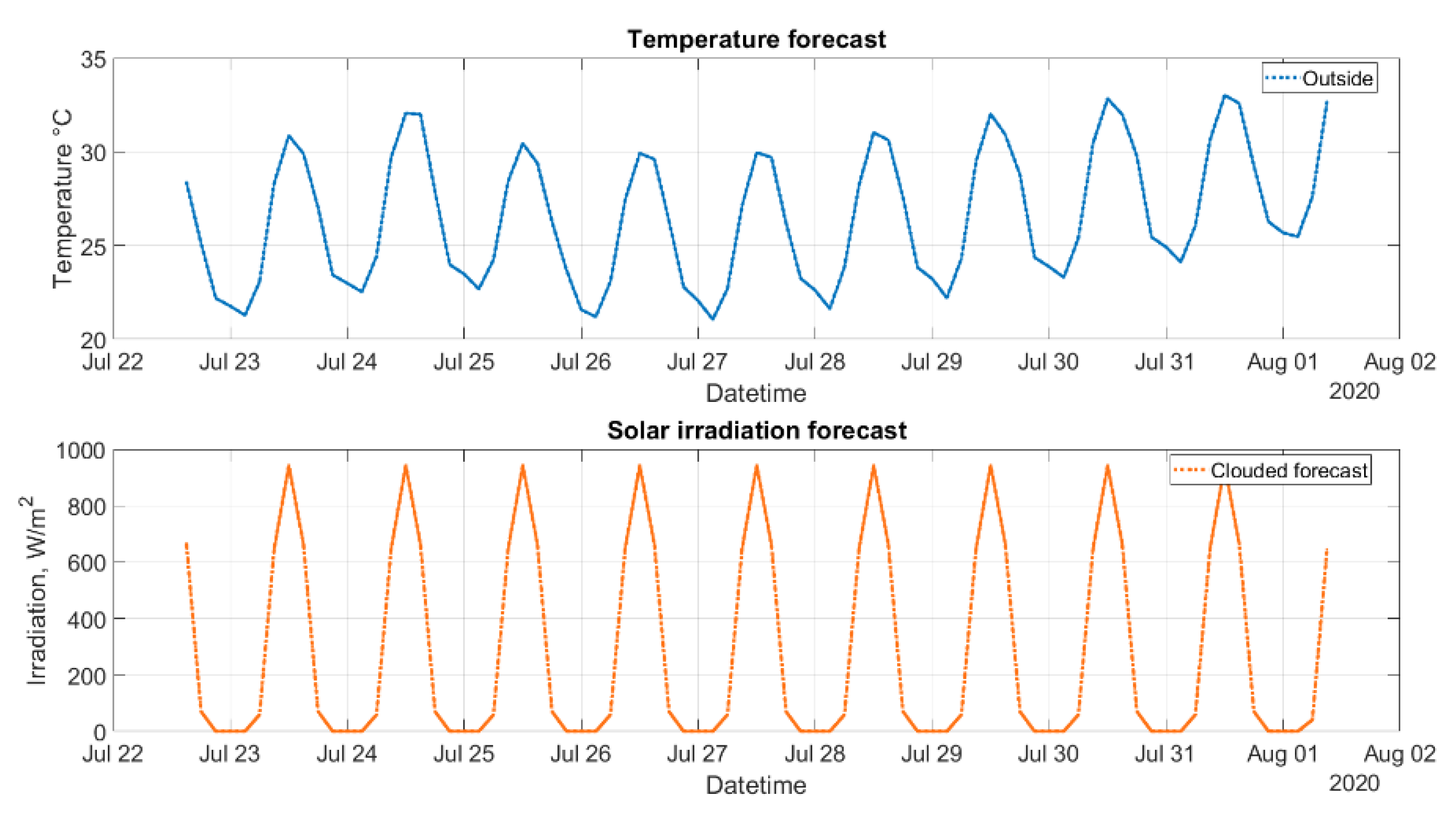
Weather forecast uses the OpenWeatherMap API, which has different types of forecasts available via a personal key that is obtained after a free registration [40]. The 5-day forecast with a 3 h timestep was used in this work. The forecast contains information about outside temperature, pressure, humidity, cloudiness, wind speed and direction, rain, and snow. The first part of Figure 8 shows the expected outside temperature for the upcoming 5 days. The second part shows the solar irradiation forecast that takes into account the expected levels of cloudiness. However, at the end of July 2020, there was no cloudiness expected, so the irradiation was not affected.

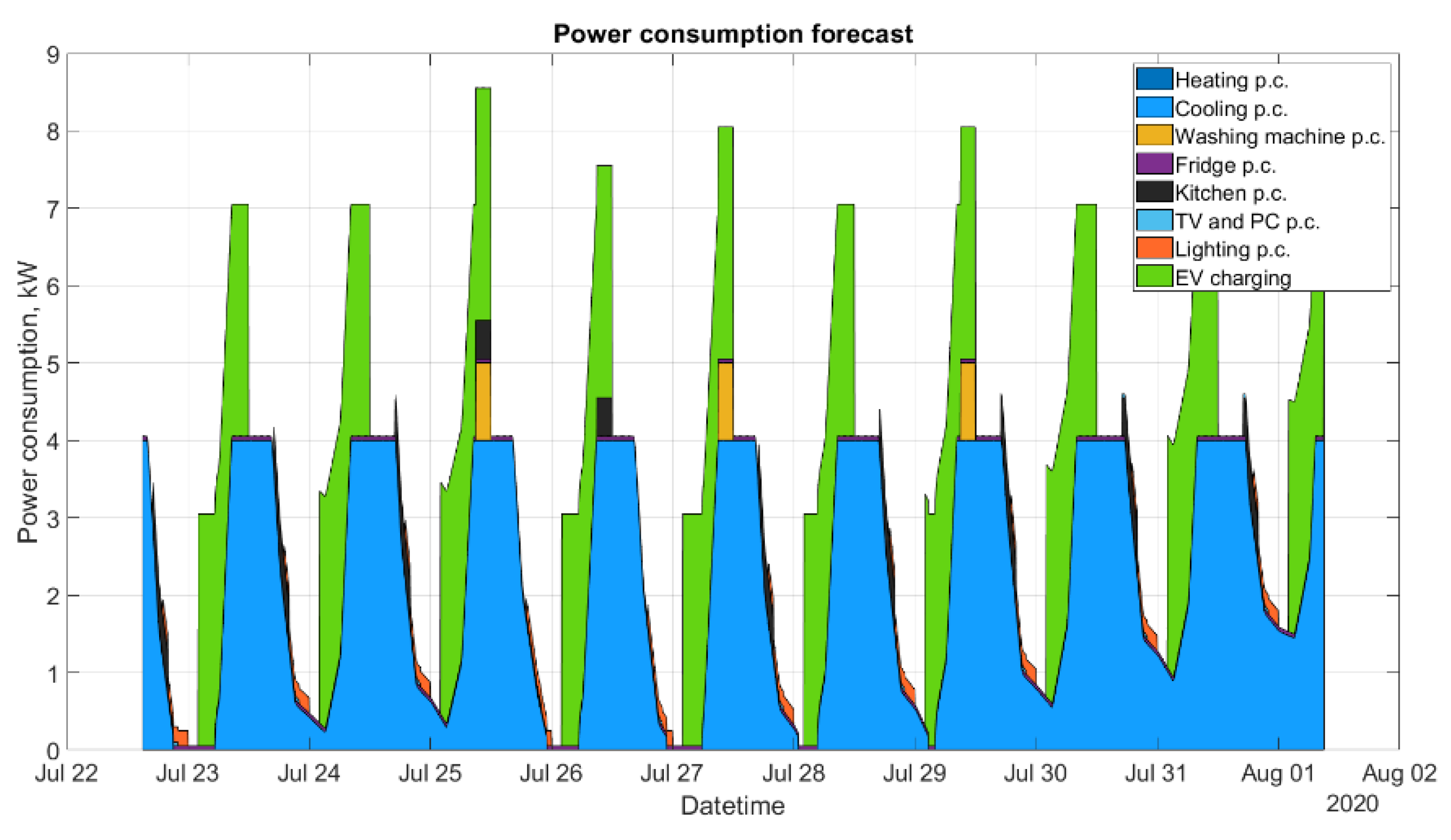
Figure 9 shows the overall power consumption prediction of each appliance as a stacked area plot.

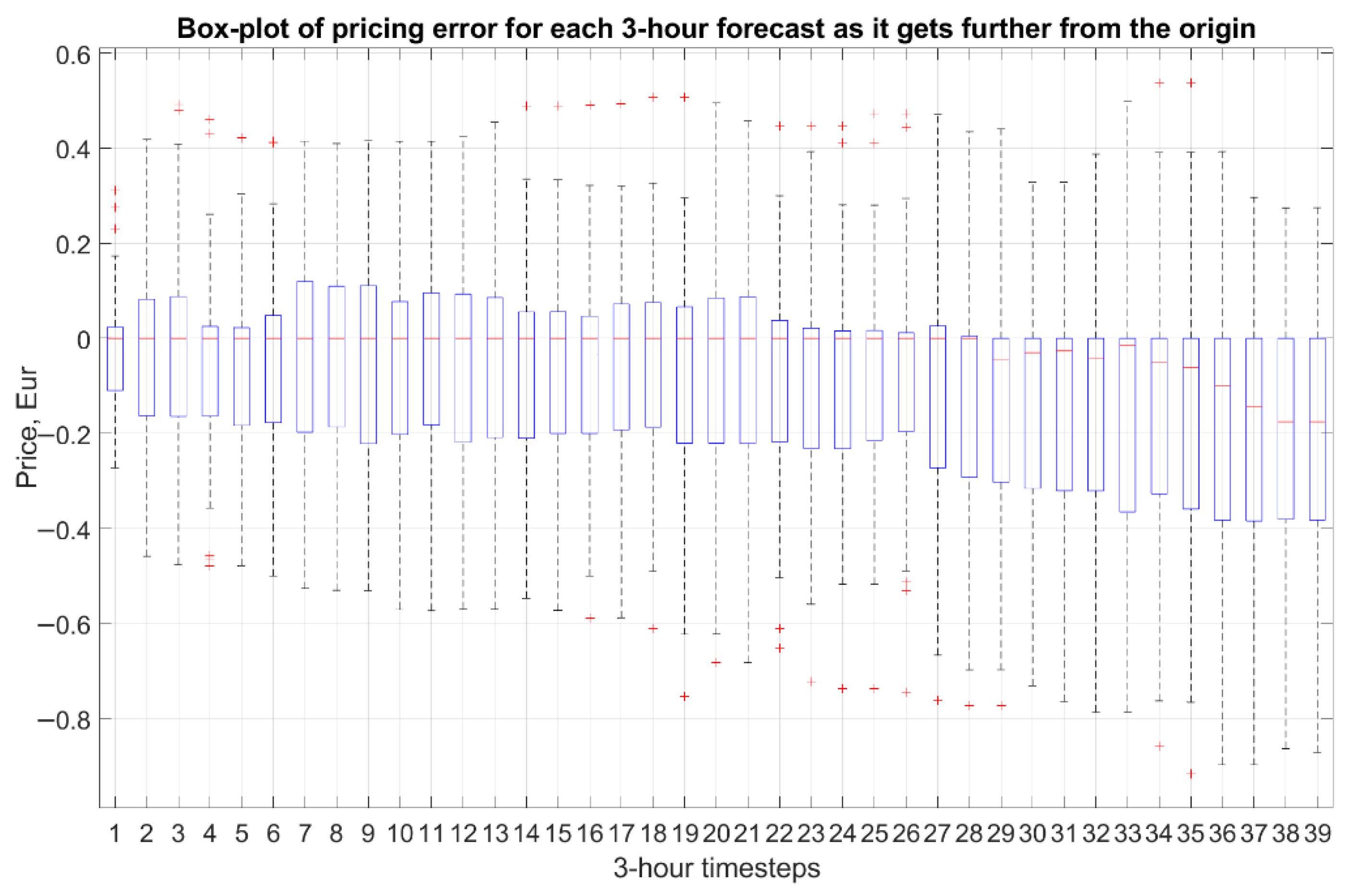
The prediction of the model’s behavior depends on the precision of the forecast. Forty weather forecasts were saved during the summer in order to make an analysis of the forecast error. The forecast with a minimal future prediction (the first forecast) was used as the real value for all other forecasts, as it was not possible to make real measurements to make the comparisons. Such error is important to understand the possible precision of the predictions and whether a 5-day weather forecast might provide any substantial valuable information. The forecasts were saved between the 22nd of July and the 30th of July 2020. The forecasts were downloaded every 3 h during these days. The total number of forecasts for comparison was 39. Because any real measurement was not available, the first forecasted value was considered the real value.

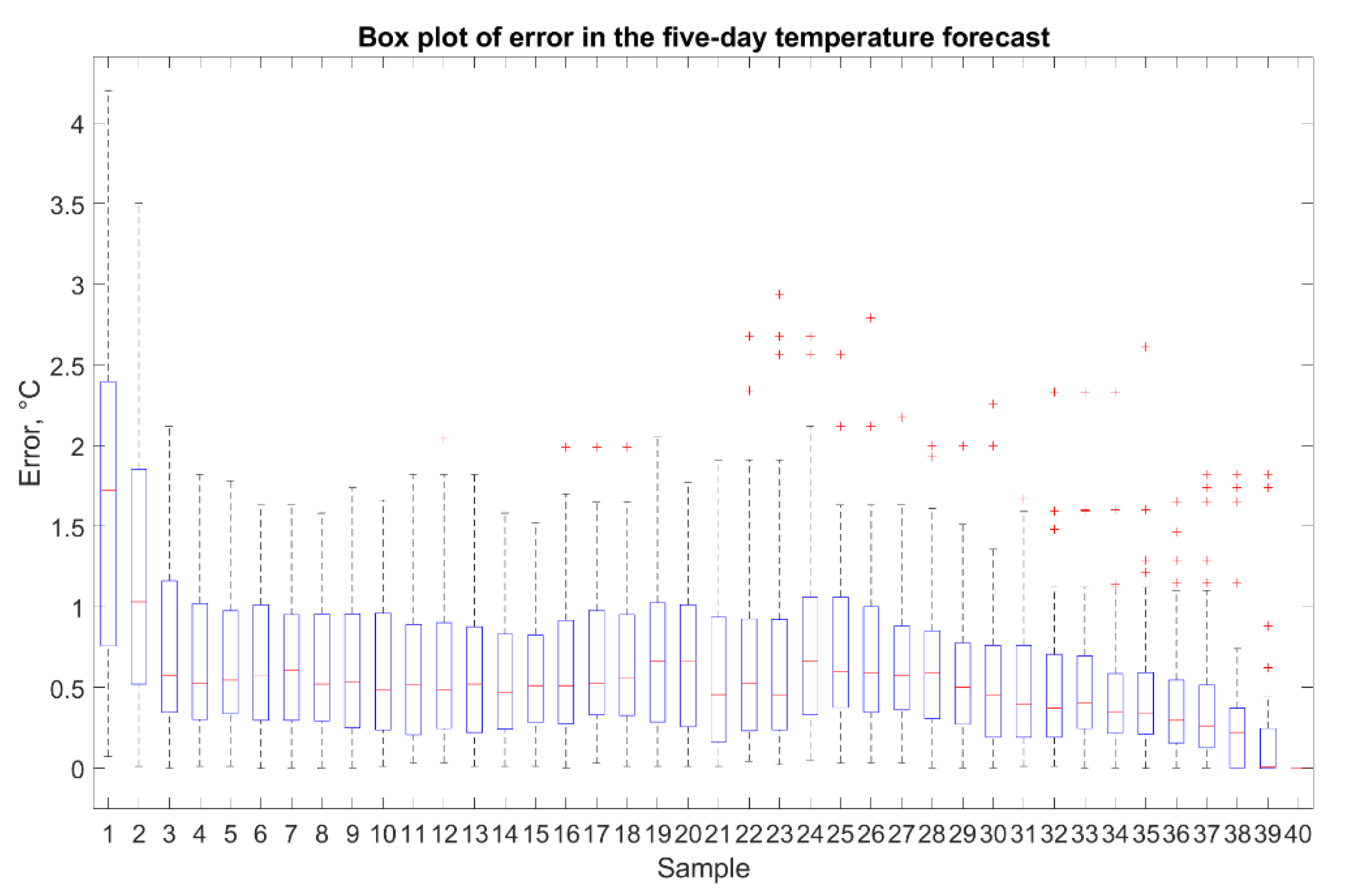
The prediction error tends to be quite large for the five-day forecasts but then the error stabilizes at a value around 0.6 °C. The changes in the error can be seen in Figure 10. which is a box plot where each box represents an error distribution for a specific time sample in all 40 forecasts.

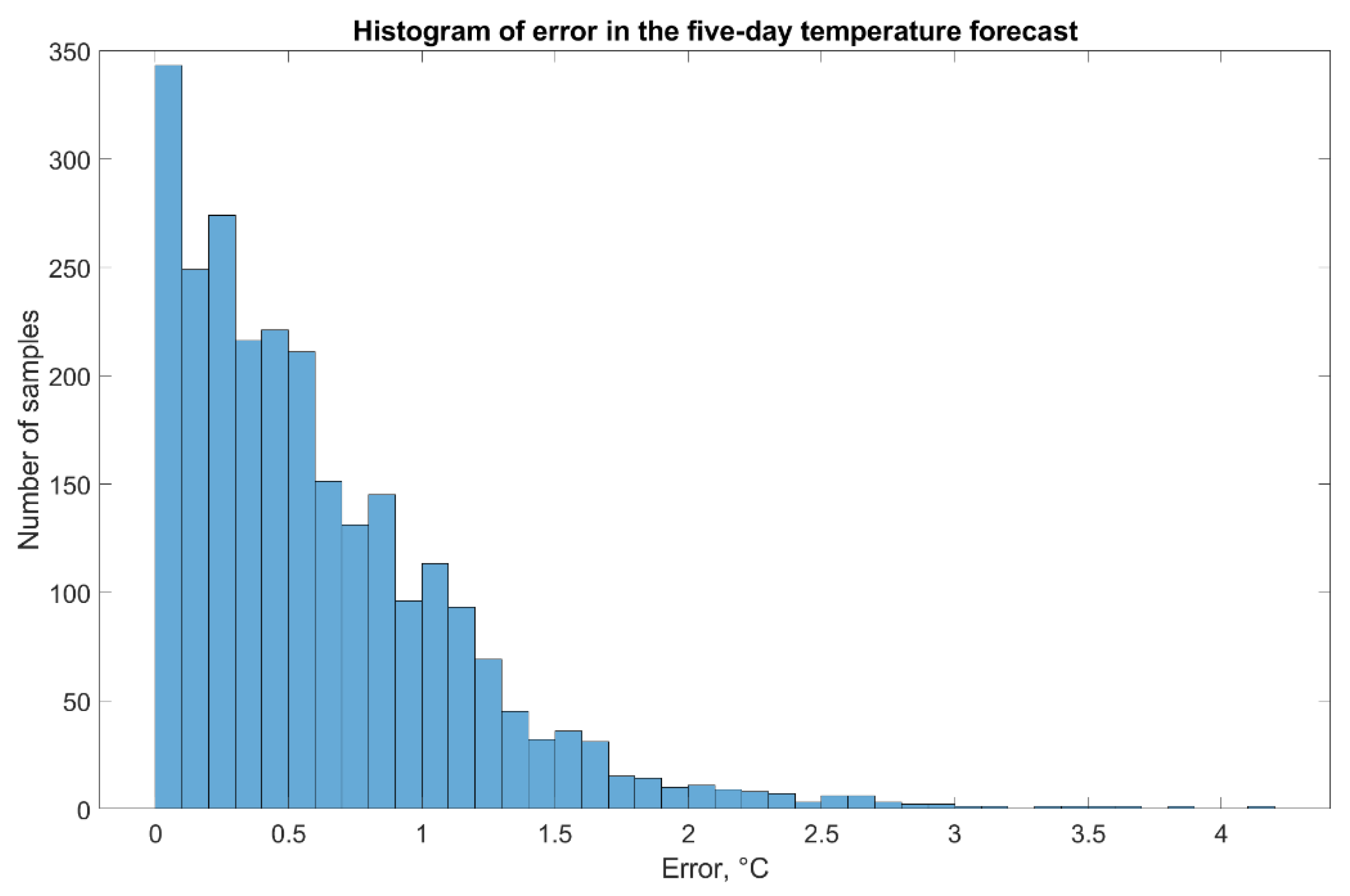
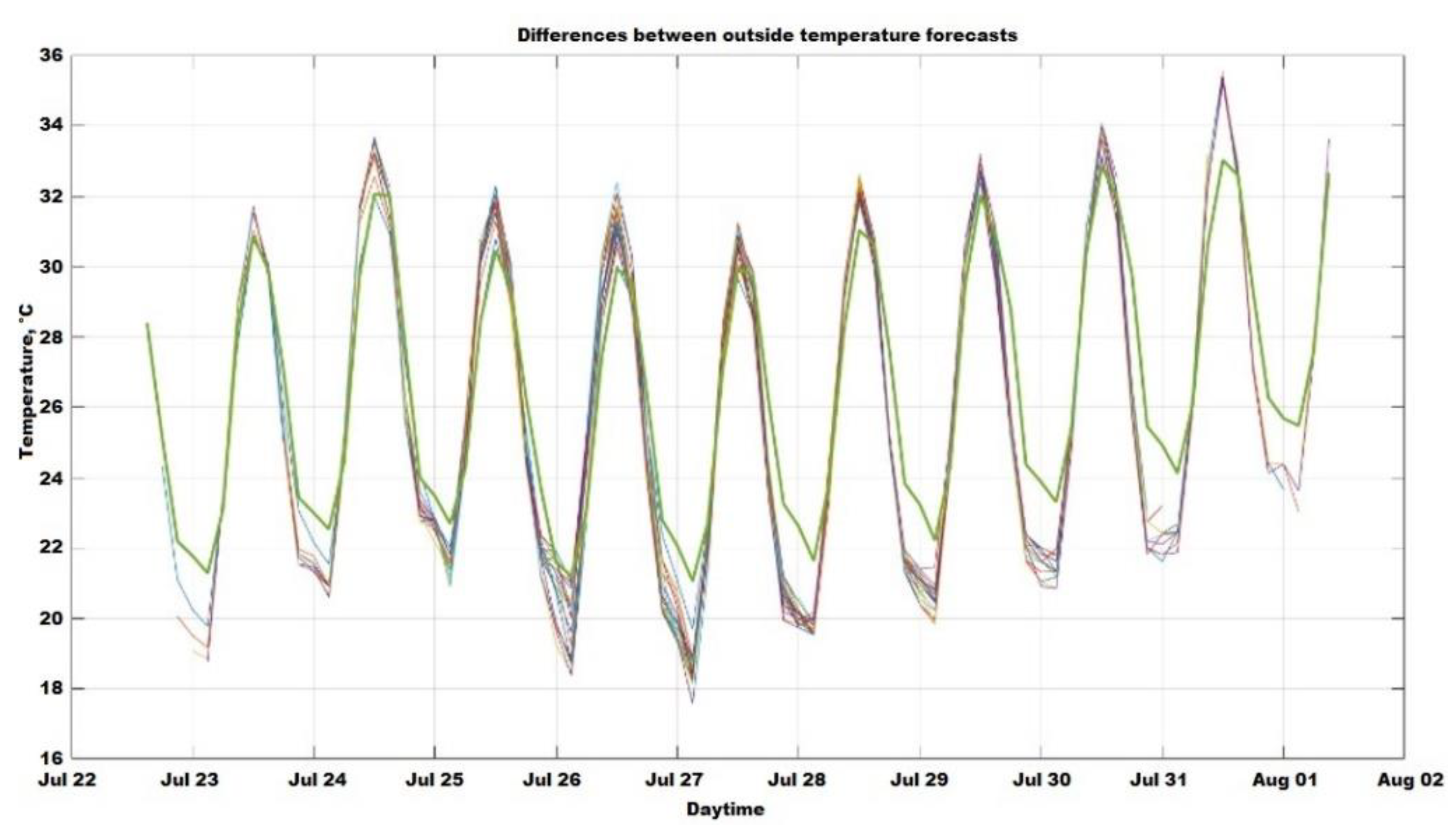
Figure 11 shows the distribution of errors. Finally, what different forecasts looked like in comparison to the first forecast (as described above) temperature can be seen in Figure 12. It shows that the forecasts have a tendency to overestimate the maximums during the day as well as underestimate the minimums during the night.

2.2. Energy Demand Prediction

The whole idea of building a model was to have suitable energy demands predictions. This paper focuses mainly on the prediction of energy costs with regard to the weather forecast and its uncertainty. Such uncertainty in the weather forecast is then translated into errors in predicted energy cost.

The pricing error was calculated in two ways: as an absolute and non-absolute value. Prices are calculated from the energy consumed for heating and cooling and such consumption depends on the weather forecast. Errors in the weather forecasts accumulate and lead to bigger mistakes in the total sum although single errors might be quite small.

The following figures are divided into two sections. The top part shows the price evolution for all forecasts with the actual price evolution. The bottom part shows the price errors that can be expected for each 3 h forecast as well as a cumulated sum of these errors.

The box plot shows the distribution of errors for each forecast. The forecasts were obtained in 3 h periods, so each box represents an error distribution for all 39 forecasts, several hours before the last, actual value. For example, the box for the 20th forecast represents an error distribution for all 39 forecasts. Each represents a 60 h ahead forecast. The cumulated sum, on the other hand, represents the sum of errors up until a certain time.

2.2.1. Absolute Pricing Error

The top part of Figure 13 shows that, during the day, the power consumption hit the maximal cooling power defined in the model. The forecasts were taken at the end of July when outside temperatures, as well as the amount of clear sunshine, are high. This power consumption is then reflected in the limited pricing levels as well. It can be seen that the biggest error occurs at night when different forecasts expected lower temperatures at night than there actually were. So, the forecasts expected a need for heating during the night.

The cumulated sum reaches an overall error of 8 EUR. This means that taking a sum of the means of all 39 forecasts leads to an expected error of 8 EUR. Although the forecasts have a tendency to overestimate power consumption, especially during the night, the forecasted pricing is higher than the actual one.

The box plot shown in Figure 14 shows the distribution of absolute errors. The mean of each error tends to be between 0.1 and 0.2 EUR for each 3 h forecast but the standard deviation gets larger the further the forecast is into the future.

2.2.2. Non-Absolute Pricing Error

When the error is not calculated as an absolute value, the graphs change as can be seen in Figure 15 and Figure 16. The cumulated sum reaches −3.5 EUR. This means that the power consumption prediction is overrated, and the actual power consumption is lower than forecasted. This overestimation occurs at each time step of the forecasts.

The box plots in Figure 16 show that the mean values of the errors tend to be close to zero but get larger as the forecasts get further, and especially the standard deviations get larger, so the forecasts become more unreliable.

2.3. Energy Demand Optimization

The biggest part of the overall energy consumption of the building is caused by heating and cooling, which correspond with the desired indoor temperature that the controller tries to achieve. An optimization strategy based on the compromise between comfort and price was implemented into the model.

The cost function is composed of two terms, namely, the deviation from the comfort temperature and the price paid for the electricity. It is expected that the owner would define the desired indoor temperature. One constant desired temperature was set for the whole horizon in the model. This defined desired temperature was then considered as the best achievable comfort. This comfort has some value for the owner, and deviating from it has a ‘price’ weighted by parameter r.

When the main aim of the optimization is to lower the price paid for the electricity consumed by the HVAC, the best result is obtained by turning off the HVAC. When comfort is of the utmost importance, then the price paid for the HVAC is defined only by the circumstances such as outdoor temperature, solar irradiance and the quality of control by the controller. If the owner is willing to make a compromise with the comfort, then the optimization finds the balance between saving money and keeping the comfort within some bounds. These bounds are defined by the user as an acceptable deviation from the desired temperature.

Such an optimization approach falls into the category of multi-objective optimization [41]. The problem of multi-objective optimization can be described as finding an optimum for a set of objective functions that are to be optimized simultaneously. This optimization problem can be generally described as

min (f₁(x),f₂(x),…,f_k(x)), subject to: x∈X

(12)

where k is the number of objective functions and X is the search space or solution space defined by constraint functions such as inequalities or equalities.

These objective functions represent conflicting objectives because improving one objective leads to degrading the other. This means that there is no single solution that would be optimal for all objective functions. A solution then consists of some trade-offs. Such a solution is called the Pareto optimal, when moving away from this solution might lead to improvement in one objective function but degrade the other [41].

It is thus clear that there is no single solution to multi-objective optimization, but rather a set of equally optimal solutions. Such a set is called the Pareto front [42]. Finding a solution to a multi-objective optimization problem can be achieved in different ways as overviewed in [41]. One possibility is to have no information about the preferences among the objectives. In such cases, the method is about finding a set of neutral compromises between the objectives. Another possibility is to subject the solutions to preferences, which can be set by the user or the decision maker before the optimization runs. These methods are called a priori. The optimization runs first and finds a set of Pareto optimal solutions from which the user or the decision maker then chooses one with regard to the preferences. This method is called a posteriori.

This work uses a weighted sum method that transforms the formulation (8) into a composite objective function [41]:

U = ∑_i=1^k w_i ∙ f_i(x)

(13)

where

w_i is the weights;

f_i is the objective functions;

k is the number of objective functions;

x is the vector of variables.

In this paper, the composite objective function is thus defined by a weighted sum formulation:

F = r ∙ ∑_k=1^N (T_{desired_by_user}(k) − T_{desired_delta}(k)) + ∑_k=1^N P(k)

(14)

where

r is the weight of comfort;

N is the number of samples from the weather forecast;

T_{desired_by_user}(k) is the desired temperature defined by the user, °C, in the k-th time step;

T_{desired_delta}(k) is the optimized desired temperature, °C in the k-th time step;

P(k) is the price paid for heating and cooling, in EUR, in the k-th time step.

In this case, the variable is the real-valued vector containing the differences of the desired temperature, T_{desired_delta}, in the time steps of the forecasting horizon:

T_{desired_delta} = [ T_{desired_delta_1}, T_{desired_delta_2}, T_{desired_delta_3}]

(15)

The price for heating and cooling is calculated by:

P(k) = p_consumed ∙ p_kWs ∙ T_s

(16)

where

P(k) is the price paid for heating and cooling, in EUR, in the k-th time step;

p_consumed is the power consumed by heating and cooling, kW;

p_kWs is the price per kWs consumed, EUR/kWs;

T_s is the sampling period, s.

The price paid for heating and cooling does not have a corresponding weight, or rather, the weight is considered to be equal to 1. This approach would fall into the category of ranking methods, a subset of rating methods, where one of the objectives is given a fixed weight of 1 [41].

As also mentioned in [41], the absolute values of the weights might not represent the actual preferences of the user because the magnitudes of each objective function might vary greatly, thus affecting the resulting composite objective function differently. In such cases, the weights might compensate for these different magnitudes of each objective function more than reflecting the preferences of the user.

The optimization calculates T_{desired_delta} so that the objective function in (13) is minimized. Two scenarios have been considered: one in which the value of T_{desired_delta} is constant for the whole forecast horizon (one variable for the optimization problem), and another in which there are three values of T_{desired_delta} used at different times each day (three variables for the optimization problem). These times reflect the presence of the residents inside the home. The value of f is calculated for the whole forecast horizon. If r is equal to 0 then the resulting change in the desired temperature corresponds to minimizing the price on the forecast horizon, so the optimization becomes a parametric optimization instead of a multi-objective optimization. Such a case shows the maximal potential for a decrease in price on the forecast horizon while the optimization is constrained to finding one or three values of T_{desired_delta_k}.

Each T_{desired_delta_k} is considered to be bounded. In this model scenario, they are bounded differently.

−4 °C ≤ T_{desired_delta_1} ≤ 4 °C

(17)

−2 °C ≤ T_{desired_delta_2} ≤ 2 °C

(18)

−3 °C ≤ T_{desired_delta_3} ≤ 3 °C

(19)

These bounds are used at different times during the days of the forecast. One is used when the user is present, another when he is not, and the third is used at night. The bounds, as well as the timings, can be set by the user and reflect the maximal distance from the desired temperature that the user is willing to accept. These bounds were considered to be fixed, but it is possible that the user’s preferences or willingness to accept discomfort might change during the day. Such changes in the preferences might be reflected in changes to the bounds as well as the weights of the weighted sum (13).

The weighted sum (13) acts as the utility function, which is supposed to approximate the user’s preference function. Such a function would represent the user’s satisfaction with changes to the value of each objective function. As mentioned in [41], the utility function used in the form of a weighted sum is a linear approximation of the preference function. However, the preference function might be non-linear, meaning the preferences might change in the criterion space, for example, if one of the objective functions reaches a certain value.

As the objective function is calculated using an iterative algorithm with non-linearities (i.e.,: constraints on the value of u), an iterative method is used for the solution of the optimization problem.

The function fminbnd in MATLAB has been used for the optimization [43]. The algorithm is based on a golden section search and parabolic interpolation [43]. This function is a one-dimensional minimizer that finds a minimum for a problem specified by

min f(x), such that x₁ < x < x₂

(20)

where

x₁ is the lower bound;

x₂ is the higher bound.

The main idea behind the optimization in this paper was to show how the predicted energy price changes with respect to different values of the desired indoor temperature. This reflects a compromise between comfort and price. The pricing range can best be shown by calculating the optimization for different values of the weight of comfort.

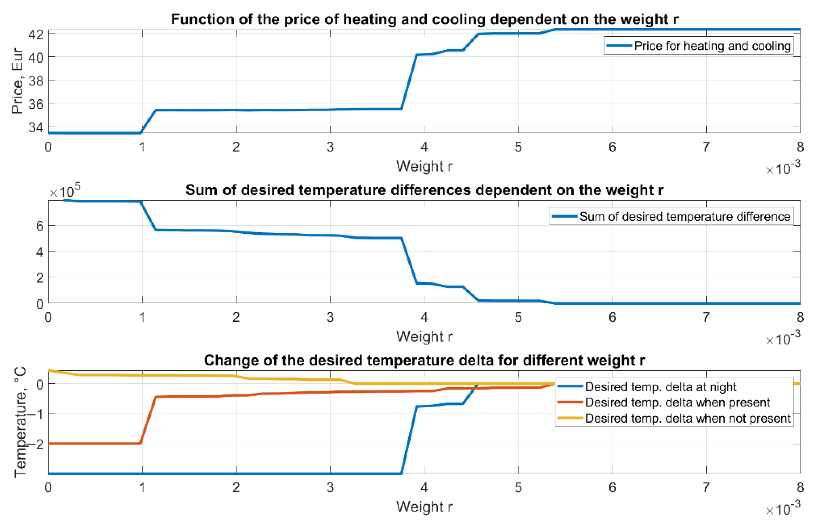
The resulting pricing range can be seen in Figure 17. It is divided into three parts. The first graph shows how the price changes with regard to the value of the comfort weight. The second graph represents a distance from the ideal comfort for different values of comfort weight. It is calculated as the sum of the difference between the desired temperature originally set by the user and the optimized desired temperature. Moreover, the third graph shows how each of the three optimized desired temperature deltas changes for different values of the comfort weight.

It can be seen that there is a compromise between the price paid and comfort. By increasing the value of the weight, comfort gains more importance, and the price rises. These graphs also show that there are 4 or 5 main areas the optimization leads to.

The desired temperature deltas in the last graph were defined as three deltas used at different times of the day. The different timings represent the times when the user is at home, and when the user is not present, and the last timing represents night-time.

The temperature delta, when the user is not present, was used during the day from 11.00 to 17.00. Its range was between −4 and +4 °C. The delta did not change very much, which was caused by the high temperatures and sunshine during the day. So, the optimization found that changing this temperature delta did not lead to a significant change in the power consumed by cooling since when increasing the desired temperature, the cooling still ran at the maximal level.

The temperature delta when the user was present was used at hours from 9.00 to 10.00 and then from 18.00 to 23.00. Its range was set to boundaries at −2 and +2 °C. When the weight was low, indicating that comfort was not important, this delta was set to −2 °C. This means that when the desired temperature set by the user was lowered to −2 °C, that would be 20 °C in the model scenario. As the weight of comfort increased, this delta lowered until it was 0 °C. In this case, the desired temperature was 22 °C, which was the same as defined by the user.

The third temperature delta was in the night-time frame and was used between 00.00 and 8.00. Its range was set to boundaries at −3 and +3 °C. This delta stayed at the value of −3 °C, resulting in the desired temperature of 19 °C for the first half of the values of the weight.

As the weight increased, comfort gained importance, which led to all desired temperature deltas being 0 °C. This is exactly the temperature that the user set as the ideal one.

The final price range obtained was from 33.44 EUR to 42.36 EUR for heating and cooling over 5 days for the modeled house.

So, such space of possible compromises could then be used for the a posteriori evaluation of a given weather forecast. The possibilities would change with the weather forecast.

A clearer example from the results would be the following. The user can take a look at the graph of the prices and the desired temperature changes for that given price. In this scenario, the user could choose to pay 35.40 EUR with the compromise of changing the desired temperature when he is present by −0.32 °C when he is not present by +0.15 °C and by −3 °C at night.

The model used in the optimization process had 10 m² of photovoltaic panels. Increasing their area or also considering flexible energy tariffs might lead to different results.

3. Results and Discussion

The quality of the model depends on the structure and parameters of the model. We chose a grey-box first-principle structure as simple as possible to be able to use the model directly in a real-time control system of a house that has limited memory capacity and computing power. Such a model must be adjusted to a specific building, and some parts of the model might need to be described with more complex relationships. On the other hand, even the accuracy of the weather forecast is not ideal, and it will influence the predictions and decisions as well.

Uncertainty in the weather forecast then leads to uncertainty in the energy demand prediction. We tested the prediction abilities of the model on weather forecast data between 22 July and 30 July 2020. The absolute mean for each 3 h forecast was around 0.1 and 0.2 EUR, which made 8 EUR uncertainty on the whole forecast horizon of 5 days. The non-absolute pricing error showed that in the period between 22 July and 30 July 2020, the energy demand predictions tended to be overestimated. The cumulated sum of the non-absolute means was −3.5 EUR.

Part of the work was focused on the possibilities of energy demand optimization via changing the desired indoor temperature. The cost function consists of the price for comfort and the price for heating and cooling. It was assumed that the user would choose the desired temperature and the times of the three regimes: presence, absence, and night-time. The optimization would then find three different deltas (each used in different time frames) by which the desired temperatures should change to accommodate the compromise between price and comfort. The cost function used for the optimization was defined as a weighted sum of the absolute deviation from the desired temperatures and the price paid for electricity. The ranking optimization method was chosen, so the deviation from the desired temperature was weighted by the weight r, and the price was given a fixed weight of 1.

The effects of changing the weight of comfort on the price and the temperature indoors are not very straightforward, as these also change with weather forecasts. The optimization was run for a range of different values of the comfort weight in order to make the possibilities of the compromise more comprehensible. These possibilities are depicted by a pricing range for different changes to the desired temperature. Such a range could then serve for a posteriori choosing of the comfort weight.

The optimization did not take into account the possibilities of pre-heating or pre-cooling. This is a topic to be investigated in future works.

4. Conclusions

The three main aims of this paper were to build a simplified mathematical model of a house that is used for the predictions of its energy demand, to calculate the uncertainty of weather forecasts (and thus the uncertainty in energy demand predictions), and lastly, to introduce an energy demand optimization model by defining the compromise between price and comfort.

The model consisted of kitchen appliances, a washing machine, a TV, a PC, and lighting fixtures. These appliances were described by their power consumption and timing during the week. The more complicated parts of the model were the heating and cooling, which were described by the energy balance with regard to the indoor desired temperature, the outside temperature, and the accumulation of energy. Another main subsystem of the model is the weather forecast. It was used to obtain the expected outside temperature and cloudiness. Cloudiness was used to create variation in the forecasted solar irradiance. Solar irradiance was also used to predict the power generation from the photovoltaic system, which then served in the energy balance calculation of the whole building. The amount of money that would be expected to be paid according to the forecast horizon was calculated from this energy balance and the prices for buying and selling the energy from and to the grid. Lastly, there is a battery subsystem for the charging of an electric vehicle. The parameters used are estimates of the expected values based on experience with similar thermal systems. The sensitivity of the predictions to model parameters was not been investigated in this paper.

This model can be used as a computationally inexpensive and scalable model for semi- or fully automated systems for the optimization of operation in residential buildings in terms of electric energy consumption. The optimization can be achieved by standard numerical methods. The feasibility of the optimization is guaranteed because of the special criteria formulation. Future work will address the testing and better tuning of the model structure and parameters, so the predictions better agree with the energy consumption behavior in real-world residential buildings. Additionally, we plan to include other important phenomena such as vehicle charge and discharge in a Vehicle-to-Home mode, or a scheduling framework based on the energy available from a photovoltaic system and a battery management system. A better indoor temperature control strategy instead of a PI controller, e.g., a model predictive control strategy, might be used to enhance the control quality as well.