Accelerated Parallel Numerical Simulation of Large-Scale Nuclear Reactor Thermal Hydraulic Models by Renumbering Methods

Abstract

Numerical simulation of thermal hydraulics of nuclear reactors is widely concerned, but large-scale fluid simulation is still prohibited due to the complexity of components and huge computational effort. Some applications of open source CFD programs still have a large gap in terms of comprehensiveness of physical models, computational accuracy and computational efficiency compared with commercial CFD programs. Therefore, it is necessary to improve the computational performance of in-house CFD software (YHACT, the parallel analysis code of thermohydraulices) to obtain the processing capability of large-scale mesh data and better parallel efficiency. In this paper, we will form a unified framework of meshing and mesh renumbering for solving fluid dynamics problems with unstructured meshes. Meanwhile, the effective Greedy, RCM (reverse Cuthill-Mckee), and CQ (cell quotient) grid renumbering algorithms are integrated into YHACT software. An important judgment metric, named median point average distance (MDMP), is applied as the discriminant of sparse matrix quality to select the renumbering methods with better effect for different physical models. Finally, a parallel test of the turbulence model with 39.5 million grid volumes is performed using a pressurized water reactor engineering case component with 3*3 rod bundles. The computational results before and after renumbering are also compared to verify the robustness of the program. Experiments show that the CFD framework integrated in this paper can correctly perform simulations of the thermal engineering hydraulics of large nuclear reactors. The parallel size of the program reaches a maximum of 3072 processes. The renumbering acceleration effect reaches its maximum at a parallel scale of 1536 processes, 56.72%. It provides a basis for our future implementation of open-source CFD software that supports efficient large-scale parallel simulations.

1. Introduction

Because of the importance of nuclear reactions and the complexity of their physical models, research exploration using large-scale numerical simulations is essential. Some early studies of nuclear reactor thermodynamics were based on several parameters at large scale or one-dimensional system analysis methods, which mainly studied the average characteristics of physical quantities in nuclear power systems. With the boom in high performance computers, nuclear power thermohydraulic studies based on more refined computational fluid dynamics (CFD) methods and thermohydraulic software have been widely studied and applied [1,2].

The internal structure of nuclear reactors is complex, and the dominant reactor type today is the pressurized water reactor. Core fuel rod bundles are an important component of a pressurized water reactor. The fuel rods are surrounded by a flowing liquid coolant. There is a violent flow of liquid between the bar bundles and between the bar bundles and the walls, and they are responsible for the transfer of momentum and heat. It is widely believed that the flow pulsations in the gap are closely related to the large-scale vortices. It has been studied that vortexes will form in pairs on both sides of the slit [3,4]. The flow and heat transfer characteristics of coolant flowing through the core of a nuclear reactor are extremely complex. To analyze the turbulent motion and thermodynamics of large-scale fuel rod bundles [5,6,7,8,9,10], large-scale CFD numerical simulations based on FVM (finite volume method) are a widely accepted solution. However, large-scale CFD numerical simulations require an extremely large amount of mesh data. The usual solution is to encrypt the mesh of the physical model. The larger the amount of data, the larger the solution size and the accuracy of the solution are naturally improved. However, this will lead to more and more complex and difficult to solve calculations. Today, the use of large-scale CFD techniques in thermal hydraulic analysis is still very difficult due to high technical requirements and shortage of computational resources [11].

In the CFD, simulation of fine flow field structures in real-world engineering cases is still forbidden [12]. As a result, there is widespread interest in improving computational efficiency by well-developed parallel technology. The CFD solving process involves three parts: pre-processing, numerical solving, and post-processing. The use of appropriate meshing methods and mesh numbering in the preprocessing process will greatly improve the computational performance of fluid dynamics simulations. Taking FVM [13,14] as an example, after meshing the physical model, assembly of linear systems in parallel from the number of grid cells of each divided component is necessary. Then, solving them iteratively. In addition, the numbering of the grid determines the order of access to the individual processes for parallel computation and affects the cache hit rate. Since modern computer architecture is characterized by multiple storage levels, reasonable grid numbering has a significant impact on the efficient utilization of computational performance.

One of the key technologies in CFD preprocessing is the meshing technique. Its theoretical basis is becoming more and more mature. In recent years, the research field of finite element meshing has shifted from two-dimensional plane problems to three-dimensional entities, and the research focus has changed from triangular (tetrahedral) meshes to quadrilateral (hexahedral) meshes, focusing on the fully automatic generation of meshes, mesh adaption and other research. Mesh partitioning can be abstracted as graph partitioning. The relationship of cells and neighbors can be abstracted as the relationship of vertices and edges. The large-scale physical model is divided into multiple blocks by coarse-grained and fine-grained lattice partitioning, which facilitates parallel computation [15]. It is a challenge to achieve high quality meshing as quickly as possible and under the condition that the load balance is satisfied. The efficiency and cell quality of meshing need to be further improved.

Another key technique in preprocessing is the grid numbering technique. The effect of grid numbering techniques on the computational efficiency of solving sparse linear systems is a classical topic with many research results, examples of which can be found in the work of Gibbs et al. [16], Cuthill and McKee [17], Sloan [18], Akhras and Dhatt [19], and George et al. are reflected in the work of Reverse Cuthill–Mckee [20]. Because the heuristic renumbering algorithm consumes a lot of time during preprocessing. Therefore, heuristic algorithms may be more appropriate when computational performance is not a critical issue [21,22]. In addition, this paper studies how to accelerate the computational performance of general-purpose CFD software, so heuristic algorithms are not considered for the time being.

In general, meshing and grid numbering techniques are a traditional approach to performance optimization, and there are many existing methods to choose from. However, these techniques still lack quantitative analysis for large-scale thermal-hydraulic cases. In particular, the optimization effectiveness for general-purpose CFD software executed on supercomputers is still lacking. Therefore, this paper focuses on the effectiveness of the FVM-based computational framework for use in unstructured grids, integrating typical meshing methods and mesh numbering techniques. Ultimately, a suitable mesh renumbering method is selected to enhance the parallel scale and computational speed of numerical simulation.

The main innovative points of this paper are as follows: (1) A general framework for further integration of parallel meshing methods and renumbering schemes in general-purpose CFD software for unstructured meshes; and (2) improved runtime speed and parallel scale for real-world numerical simulations of large-scale complex cases. The case is a thermal hydraulic analysis of a 3*3 fuel rod bundle with 39.5 million grid volumes.

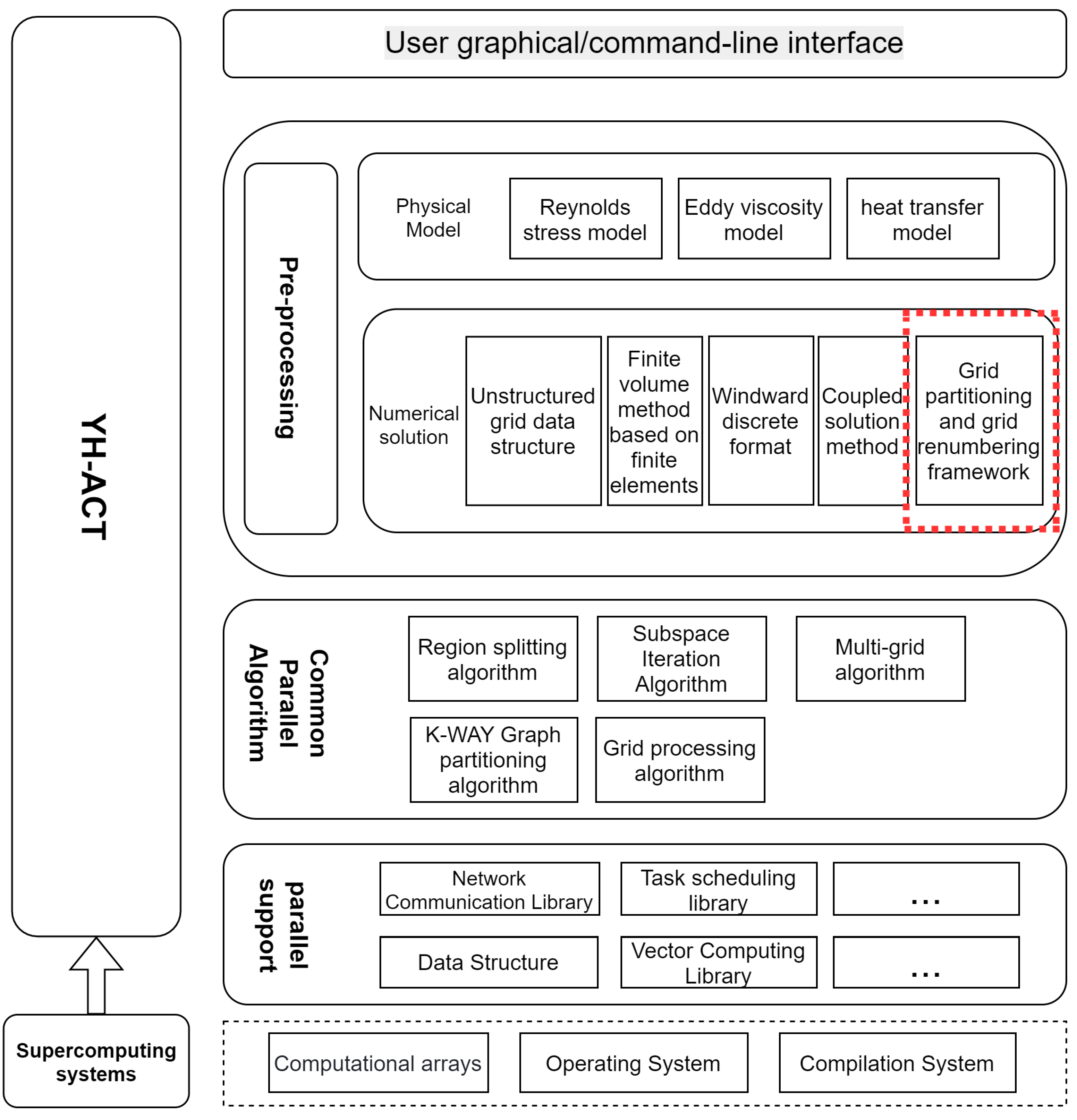
The structure of this paper is as follows: Section 2 describes the generic CFD software used in this paper and aims to demonstrate the advantages of the software between data structure and parallel communication. Section 3 shows the meshing strategy and the integrated RCM renumbering algorithm. Section 4 demonstrates the correctness of the massively parallel numerical simulations before and after renumbering and the huge improvement of the renumbering algorithm on the numerical simulation efficiency. Conclusions are included in Section 5.

2. General CFD Software Based on Finite Volume Method

The general-purpose CFD software used in this paper, YHACT, was initially used for thermal-hydraulic analysis. YHACT uses a modular development architecture based on scalability. It is based on a framework blueprint of CFD program modules consisting of key steps in CFD solving such as data loading, physical pre-processing, iterative solving, and result output. YHACT mainly addresses the thermal-hydraulic CFD program requirements for nuclear reactors, and more details about it can be found in [23].

2.1. Scalability of YHACT Software Architecture

Thanks to the modern features of object-oriented technology, YHACT can be developed modularly and has flexible scalability. YHACT is based on common parallel algorithms and parallel support, combined with existing advanced software engineering methods. It uses physical model module, numerical discretization module, linear equation system module, and parallel communication module as the main components to form the general framework of CFD program based on supercomputing system [24].

The pre-processing toolbox has functions such as mesh control and physical pre-processing. The physical model and numerical solution constitute the CFD solver, encapsulating the physical mathematical model and efficient mathematical solution methods with parametric configuration capabilities. The common algorithm implements parallel computation such as sparse iterative methods and preconditioners. Through close coupling with the computer architecture, YHACT can obtain support for massively parallel computational optimization and provide fundamental computational power for the solver. Parallel support can encapsulate the structural features of high-performance computer systems and provide fundamental computing, communication, storage, and debugging functions, thereby supporting the efficient operation of large-scale CFD computing applications. Therefore, the good scalability of YHACT makes it easier to integrate meshing techniques and mesh rearrangement schemes. As shown in Figure 1, it does not require much change to the software architecture, but only requires the implementation of the required functions by calling the interfaces of each module. The overall framework of the grid partitioning technique and grid rearrangement scheme will be presented in Section 3.

2.2. Parallel Solving Algorithm

2.2.1. Parallel Decomposition of Grid Data

A simple and intuitive way of parallelism is to decompose the grid data. Similar to Cartesian partitioning, the grid data are divided into as many copies as required and then distributed to different processes for computation. The processes rely on communication to exchange data between them.

The data decomposition is shown in Figure 2. The grid to be solved is divided into non-overlapping blocks of grid sub-cells, and each process reads only one piece of grid data. After data decomposition, dummy cells are generated on the physical boundaries adjacent to each sub-grid and other grids for data communication only. Dummy cells are only used for data exchange and are not part of the physical model, which makes each cell consider only the data of its neighbors. The data on the dummy cell can be used as boundary data. This simple data decomposition does not share the grid data. In addition, a discrete format of up to 2nd order is used, and only the values of adjacent grid cells are used in the grid calculation. Therefore, the cross-process data to be acquired can be stored on the boundary line (dummy cell in Figure 2). The solution can be divided into the following three steps: (1) boundary initialization (fetching data on adjacent processors); (2) process local computation; and (3) boundary update (updating data on adjacent processors).

2.2.2. Communication Patterns after Parallel Decomposition

Since each grid block only needs to communicate with its neighbors. The first step in establishing the communication relationship is to find all the neighboring grid blocks and store them in the local array. Each grid block then only has information about itself and its neighbors, which are “localized” grid blocks. When the parallel scale increases, the current grid only needs to traverse the “localized” grid blocks when communicating, which greatly improves the efficiency of communication. MPI asynchronous communication is also used to further improve communication efficiency. An example of a communication model is shown in Figure 3.

2.2.3. Parallel Architecture Based on MPI and OpenMP

Based on the grid model decomposition described above, two or more levels of data partitioning can be carried out. Depending on the computational resources or data structure, a certain number of “sub-grids” can be used as input to a process to perform computation. A hybrid MPI/OpenMP parallelism mode can be used. MPI parallelism is used on the first-level partition, and then the first-level partition is divided into several second-level sub-partitions. The number of second-level sub-partitions is generally equivalent to the cores inside the compute node. Coarse-grained OpenMP parallelism is performed on the second-level partition.

This multi-tier parallel architecture is adapted to the current architecture of supercomputer clusters, where primary partitions are assigned to individual compute nodes, while secondary partitions are on top of the same compute node. The above is also applicable to heterogeneous systems. The first layer still uses MPI communication based on the grid’s first-level partition interfacing information. The second layer is OpenMP parallelism, i.e., coarse-grained parallelism between compute cores, based on secondary subpartitions of the grid. Data transfer between CPUs and coprocessors is performed using the corresponding channels. When there is no coprocessor, the above heterogeneous parallel mode automatically degenerates to homogeneous parallel mode. In order to provide better control over the different partitioning layers, the whole computational domain is divided into two layers: Layer 1 is the Region partition and Layer 2 is the Zone sub-partition. In parallel computation, the Region partition is assigned to a compute node, corresponding to an MPI process, and the Zone subpartition is assigned to a compute core thread, corresponding to an OpenMP thread.

A typical CFD solver execution process mainly includes residual initialization, time step calculation, flux calculation, time advancement, flow field update, and intersection communication. The solver is applied to the computational domain Zone. For different physical models, multiple solvers may be loaded on a Zone. During the computation, Region traverses each of these Zones in turn, calling the corresponding solver to perform the computational task. When OpenMP parallelism is used, the computational tasks can be performed concurrently for each Zone.

2.2.4. Parallel Communication for Data Packaging

In the multi-level parallel architecture described above, there may be multiple subgrid blocks on each MPI process. If we directly follow the above model of cyclic traversal of grid blocks for MPI/OpenMP hybrid parallel communication, there will be the problem of multiple communications between processes. Take Figure 4 as an example, Region0 and Region1 have 2 sets of adjacent subgrid blocks, and each exchange of data requires two send and receive processes. Therefore, the grid partition data between processes can be packaged as shown in Figure 5 to reduce the number of communications.

3. A General Framework for Grid Partitioning Techniques and Grid Renumbering Methods

3.1. Parmetis-Based Grid Partitioning Strategy

Metis and ParMetis are tools that work on physical model partitioning. Usually, using the Metis library for mesh slicing of physical models using a serial strategy is an ideal solution. However, it is slow under large-scale mesh partitioning. ParMetis is a parallel version of Metis, an MPI parallel library. It has many built-in algorithms for mesh partitioning and repartioning of unstructured graphs.

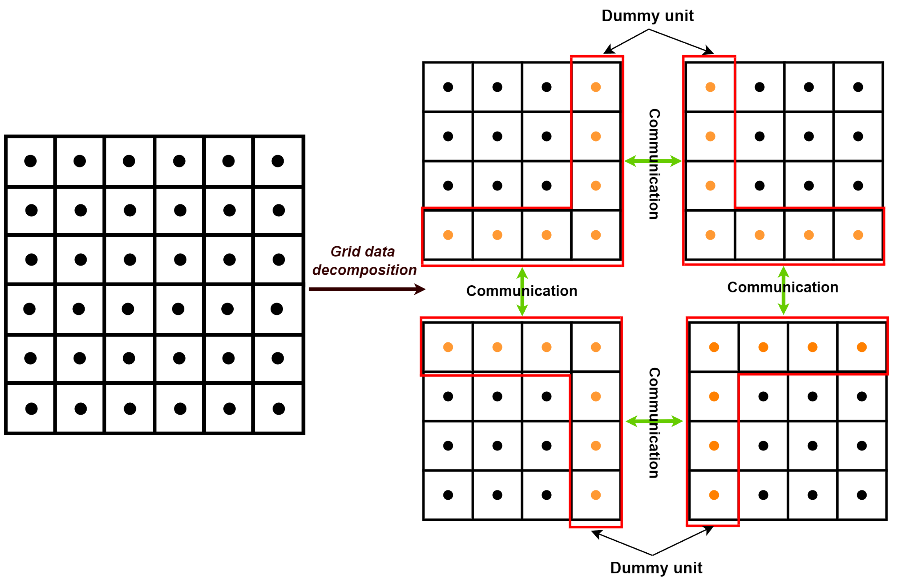
ParMetis started out as a tool for large-scale graph partitioning, but mesh models in CFD can also be abstracted to graphs. Therefore, ParMetis is particularly well suited to deal with unstructured meshing problems in large scale numerical simulations. Simulations of fluid problems often require thousands of cluster nodes to be computed simultaneously. Before the computation, a regional decomposition of the computational grid has to be performed. Communication is required between different regions in the computation. Therefore, grid region decomposition has a greater impact on load balancing and inter-process communication. PartMetis enables the partitioned area grid to be approximately the same and the number of intersections to be minimized. Therefore, the amount of data exchanged is minimized, which in turn significantly reduces the communication time between processes.

ParMetis provides the ParMETIS_V3_PartGeomKway routine for computing partitions of graphs derived from finite element meshes where vertices have coordinates associated with them. Given a graph distributed between processor and vertex coordinates, ParMETIS_V3_PartGeomKway uses the space-filling curve method to quickly compute an initial partition. The graph is redistributed according to this partition and ParMETIS_V3_PartKway is then called to compute the final high quality partition. Information about the partitioning process of Parmetis is available in [25].

3.2. Grid Renumbering Framework

The neighbor relationship between adjacent cells reflects the memory access order of the numerical simulation. The system of discrete equations is obtained by discretizing on each interval of the control volume of the entire domain to be solved. Discrete systems of equations are presented as sparse matrices in a computer [13], where the non-zero elements of each row denote the coefficients of the unknown quantities of the current set of equations. The matrix usually contains a few nonzero elements, and the number of non-zero elements is exactly equal to the number of elements associated with this row.

For different grid types, the coefficient matrix of a structured grid is banded, while the coefficient matrix of an unstructured grid is relatively irregular and only has the characteristics of a diagonal matrix. Therefore, based on the above characteristics, many solutions have been proposed. The methods for solving large-scale equations can be divided into direct and iteration approaches. Since the real case grid size of thermal hydraulics is usually large, the solution process of direct method requires a large amount of computational resources and the cost of solving the inverse is very high. Therefore, iteration approaches are usually used to addressing massive thermal-hydraulic problems. The iterative method means that the algorithm needs to be used several times to reach a convergence state. For example, ILU decomposition method, and the conjugate gradient method can be used as representatives of the iterative method for solving.

The key to improving the speed of solving is that, by writing part of the memory data to the cache, the solver can access the required solved data with higher efficiency. In other words, by rearranging the mesh without altering the program structure [26], more valid data can be written to the cache to prevent frequent memory reads for a higher cache hit rate. Therefore, this section integrates part of the grid renumbering framework in YHACT, including but not limited to the Greedy algorithm and CQ algorithm implementation, which can be found in [27], and the RCM algorithm is elaborated below.

3.2.1. RCM Algorithm

After careful algorithm design, the RCM algorithm was shown to be able to adapt to large-scale distributed memory parallelism [28] and has been widely used in software such as OpenFoam and MatLab. When the numerical stage of sparse matrix computation is reached, the matrix is usually distributed. At this point, the RCM algorithm can improve the sparse structure of the sparse matrix, making the non-zero elements more concentrated, which can theoretically improve the storage efficiency of the computer.

The RCM algorithm uses BFS to traverse the nodes in the graph. At each layer of the graph, nodes are sorted according to their degree labels for the renumbering of that layer. In this paper, due to the modular nature of the numerical simulation framework and the complexity of the case, the algorithm’s feature of sorting nodes according to their degrees is weakened to reduce the time cost of partially traversing the nodes. Algorithm 1 shows the overall program structure.

Algorithm 1 RCM numbering algorithm

input:$mes{h}_0$

output:$mes{h}_n$

1: Select the initial unit to be numbered, set to $mes{h}_k$. Set its number to the value of the maximum number of units

2: Arrange the unnumbered neighbors of $mes{h}_k$ in the container L according to the descending order of degree

3: Set the first element of L to $mes{h}_k$ and renumber it. The value is the maximum number of cells minus one

4: Implementation Step 2

5: Implementation of step 3, and the numbered values in decreasing order

6: Repeat until the numbering is complete

Note that the initial numbered cells of the original RCM algorithm are selected by traversing the entire grid of the computational solution domain. The degree of meshes is used to achieve the desired optimization. Here, we require that the initial elements be selected as boundary cells or close to the boundary. This method prevents excessive time overhead due to the large and complex size of the case. It makes the algorithm more adaptive in increasingly complex cases. The key step is the numbering. The RCM algorithm sorts the meshes in reverse according to the sequence of degrees, from “nElement -1” to “0”.

3.2.2. Selection of Grid Renumbering Methods

Usually the sparse structure of the generated sparse matrices will vary for different renumbering methods. Bandwidth and profile are two common methods to discriminate the quality of sparse matrices. In the computer’s storage structure, the sparse matrix eventually participates in the CFD solver computation, and its sparse structure has a significant impact on the cache miss rate during the computation, which in turn affects the computational efficiency of the numerical simulation. Nevertheless, the above only represents the sparse structure of the matrix as a whole and ignores the degree of aggregation around the diagonal elements of the sparse matrix. The more elements close to the diagonal, the smaller the cache miss rate will be. Therefore, this paper adopts the MDMP discriminant method, and more details can be found in [27]. This ensures that more data are hit in the same cache:

The MDMP discriminant formula is:

$$\overline{d}=\sum _{k=1}^{\frac{n}{2}}\frac{d_k}{k}$$

(1)

It has been shown that the MDMP metric can describe the dispersion of this sparse matrix very well.

4. Parallel Experiments for Numerical Simulation of Large Scale Nuclear Reactor Thermodynamics

This section runs a typical configuration on a high performance machine in modern times. The computer consists of about 120 computing nodes. Details of the HPC are shown in

Table 1. The platform configuration used in the study.

Parameter	Configuration
Processor model	Intel(R) Xeon(R) Gold 6240R @2.40GHz
Number of cores	48 cores
Memory	192G
OS	Red Hat 8.3.1-5
Compiler	GNU Compiler Collection (GCC 8.3.1)

. The hardware configuration CPU is an Intel(R) Xeon(R) Gold 6240R processor with 48 cores and 192G RAM.

4.1. CFD Physical Modeling of Nuclear Reactor Thermal Hydrology

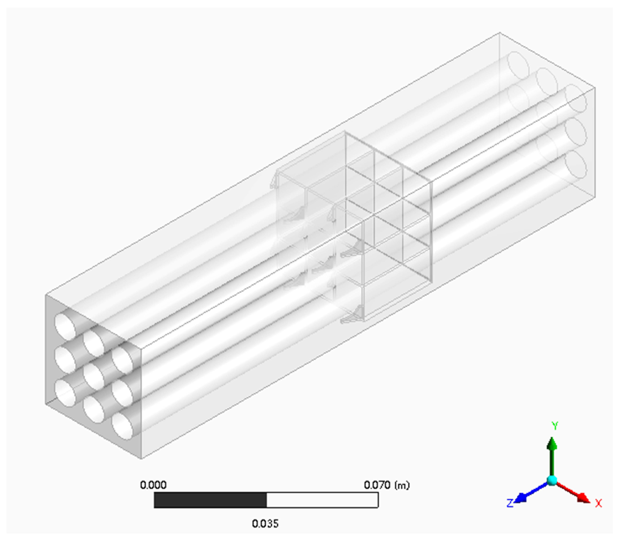
In the process of nuclear reactor thermodynamic analysis, the flow of coolant heat transfer process needs to be modeled. Figure 6 illustrates the thermal hydraulic model of a nuclear reactor that is the main focus of this paper. The theoretical model needed to completely describe the flow in the fluid as well as the heat transfer process contains three types of conservation equations for mass, momentum and energy [29].

The structure inside the pressure vessel is complex, the range of flow scales is large, and the practical application of engineering is more concerned with the average amount of physical quantities. Therefore, Reynolds averaging is generally performed for the three major equations to calculate the average physical quantities of fluid flow. In addition, then the turbulence model needs to be added in order to make the averaged mass, momentum and energy equation set closed. This is used to perform simulations of core cooling fluid flow and heat transmission. Therefore, for the thermodynamic model, a smaller grid size will lead to insufficient accuracy of its simulation. Therefore, in this paper, a 3*3 assembly with about 39.5 million grid size is simulated numerically for a fuel rod bundle. The SIMPLE iterative algorithm and PETSc solver are used to perform the calculations. The relevant parameters of the calculation, such as the relaxation factor, are adjusted. Pressure relaxation factor and velocity relaxation factor are set to 0.3 and 0.5, respectively, and a turbulence physical quantity relaxation factor of 0.5 are used to calculate the turbulent flow between fuel rod bundles with stirred wings.

It is worth noting that YHACT currently mainly considers the implementation of the Reynolds time-averaged turbulence model. As for the fluid–solid coupled heat transfer model, the heat transfer model between fluid–solid domains is generally established through the intersection of fluid and solid domains. When calculating the energy equation in the solid domain, the relevant physical quantities at the intersection of the fluid domain are used as boundary conditions. In addition, when calculating the energy equation in the fluid domain, the heat (temperature) distribution at the solid intersection is used as the source term of the fluid energy equation to finally realize the coupled fluid-solid heat transfer. Since this paper mainly concentrates on the turbulent heat transfer model, the solid models of fuel rod and control rod are neglected. The boundary condition of the solid interface on the pure fluid is a fixed heat flux. This heat flux is roughly calculated based on the solid bar size and the volumetric heat source at the time of fluid–solid coupling.

4.2. Select the Grid Renumbering Algorithm

This subsection focuses on how to select the appropriate grid renumbering algorithm. Based on the integrated renumbering strategy, the sparse structure of the sparse matrices generated by each type of grid renumbering is discriminated by MDMP metrics for the above fuel rod bundle model. Finally, the most suitable algorithm is selected for numerical simulation.

Due to the large grid size, it is more difficult to obtain the grid numbering geometry information of the physical model by serial means. Therefore, this subsection collects the numbering geometry information of the subgrids in process 0 for the two parallel scales of 48 and 96 processes to determine.

Table 2. The sparse matrix of the grid after being processed by different renumbering algorithms. The blue dots indicate the non-zero elements in the matrix.

Numbering Strategy	48 Process	96 Process
original
MDMP	32,387.88	16,588.94
RCM
MDMP	44.61	44.35
greedy
MDMP	55.24	54.16
CQ
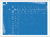
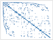
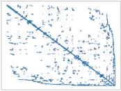
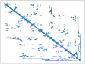
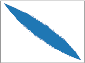
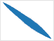
MDMP	838.29	378.98

shows the sparse matrices generated by four different numbering methods for each of the two parallel scales. Below, each row of the sparse matrix corresponds to its MDMP index.

A simple comparison can be made to conclude that the original numbering of the grid drawn by the ICEM library is confusing. After renumbering, the properties of the sparse matrix are better improved. Meanwhile, the RCM algorithm will be better compared to several other numbering methods. Therefore, in the following parallel tests, the RCM renumbering algorithm is chosen.

4.3. Massively Parallel Performance Testing

4.3.1. Proof of Correctness

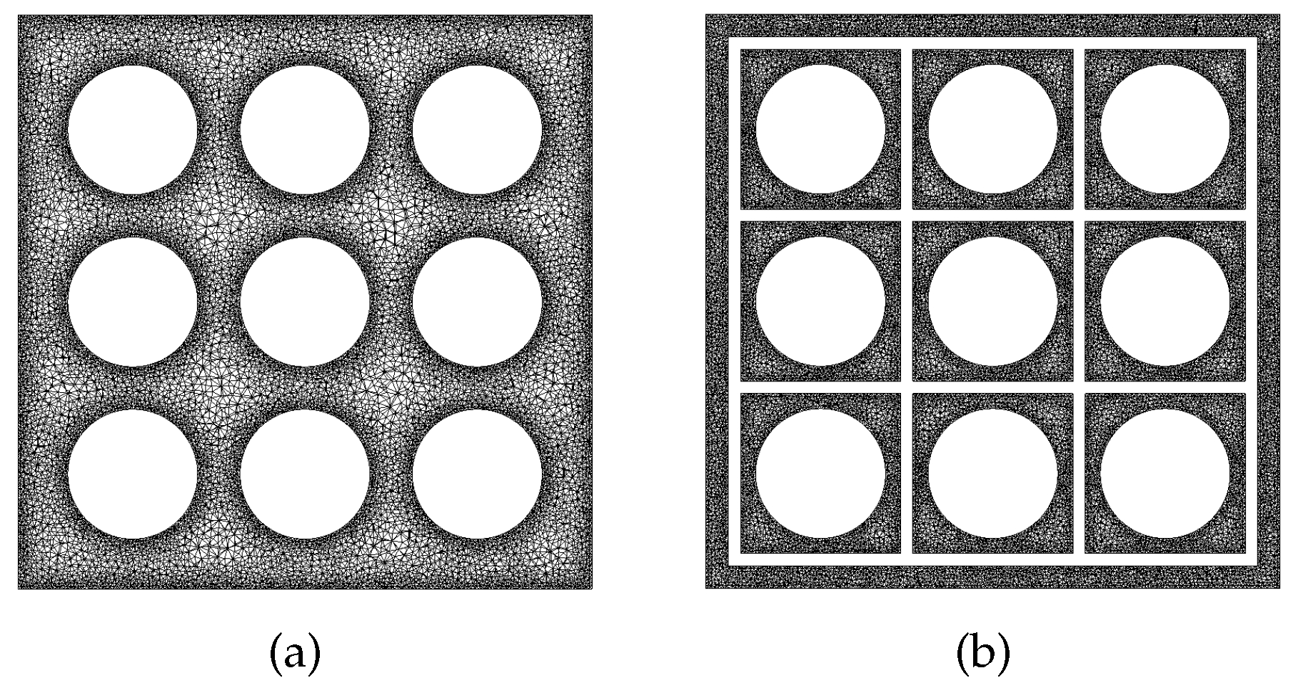
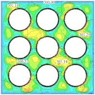
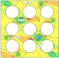
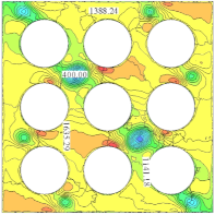
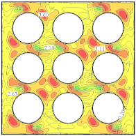
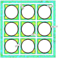
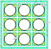
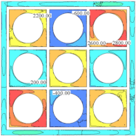
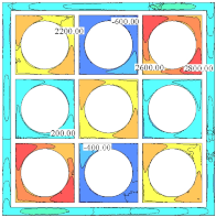
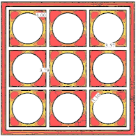
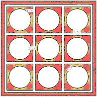
Parallel performance tests must ensure the correctness of the numerical simulations. After optimization by renumbering the modules, proof of program robustness is essential. Figure 7 illustrates the two slice models tested in this subsection. (a) shows the slice with Z = 0.01, (b) shows the slice with Z = −0.01. In addition, (b) belongs to the shelf section, which has more complex physical properties.

Table 3. Contour clouds for slices with Z = −0.01. The first column indicates the different physical quantities. The second column indicates the range of physical quantities in the cloud map. The third and fourth columns show the sliced clouds at the same locations before and after the renumbering algorithm. The white numbers in each cloud represent the values of physical quantities at the current position. When the same physical quantities are compared, both numbering methods take the same position.

Physical Properties	Range	Old	RCM
Temperature
Pressure
Velocity

and

Table 4. Contour clouds for slices with Z = −0.01. The specific information is the same as the legend in Table 3.

Physical Properties	Range	Old	RCM
Temperature
Pressure
Velocity

show the profile cloud plots for the slice at Z = 0.01 and the profile cloud plots for the slice at Z = −0.01, respectively, for comparing the correctness of the numerical simulations before and after renumbering. Each table shows the contour plots of temperature, pressure, and velocity. The first column represents the different physical quantities. The second column represents the range of physical quantities in the cloud plot. The third and fourth columns show the sliced cloud plots at the same locations before and after the renumbering algorithm. The white numbers in each cloud represent the values of physical quantities at the current position. When the same physical quantities are compared, both numbering methods take the same position. Therefore, the corresponding positions of the white numbers before and after renumbering are the same. The white numbers in the cloud plot are the values of physical quantities at the same locations, which are used to determine whether the accuracy of the renumbering optimization meets the requirements and whether the robustness of the program is guaranteed. It can be seen that the renumbering does not change the correctness of the numerical simulation either at the fuel bar (Z = 0.01) or at the shelf (Z = −0.01). The robustness of the procedure is guaranteed.

4.3.2. Parallel Testing of Large-Scale Numerical Simulations

Finally, in this paper, parallel numerical simulations are performed for a fuel rod bundle of 39.5 million grid size with a different number of processes.

Table 5. The degree of enhancement of the RCM algorithm for numerical simulation of fuel rod bundles at different parallel scales. The first column represents the number of nodes. The second column represents the amount of processes. The third and fourth columns indicate the total simulation time for the original grid and the grid renumbered by RCM. The fifth column indicates the numerical simulation speedup of the renumbered grid compared to the original grid.

No. of Nodes	No. of Processes	Time		Speedup Rate
		Original(s)	RCM(s)
2	96	19,731.4	13,682.5	30.66%
4	192	8635.3	6727.38	22.09%
8	384	3761.11	3342.41	11.13%
16	768	1794.29	1568.07	12.6%
32	1536	1618.58	700.528	56.72%
64	3072	748.43	716.175	4.31%

shows the time to iterate 100 steps on different processes for the original grid and the grid renumbered by RCM. The first column represents the amount of nodes used. The second column indicates the number of processes used, trying to ensure that each node is used 100%. The third and fourth columns indicate the total simulation time for the original mesh and the RCM renumbered mesh. The fifth column indicates the speedup of the numerical simulation of the renumbered grid compared to the original grid. It can be obtained that the renumbering module has a good effect on the computational effectiveness of the mathematical simulation of the fuel rod technique. In addition, the parallel scale reaches a maximum of 3072 processes. At the parallel scale of 1536 processes, the renumbering module has the maximum speedup effect of 56.72%. In addition, at the parallel scale of 3072 processes, the time difference is not much. This may be due to the fact that, when the grid size is certain, the larger the parallel scale, the matrix computation time within the processes decreases dramatically, while the percentage of communication time increases dramatically.

5. Conclusions

In this paper, we focus on how to apply suitable renumbering algorithms to enhance the performance of large-scale nuclear reactor fuel rod technology in a CFD numerical simulation framework. We do this by further integrating the meshing and mesh renumbering framework of YHACT, a general-purpose CFD software. The RCM algorithm is easily implemented by relying on the modular nature of the software. In this paper, we first perform parallel meshing of the model using Parmetis to ensure that each process obtains a similar size of mesh blocks and thus try to ensure that the computation time of each process is not significantly different. In addition, then, through rigorous experiments, we use MDMP as the discriminative index of sparse matrix quality to select a more suitable renumbering algorithm for the experimental case of this paper. Through the MDMP metric, it is easy to select the RCM algorithm is what we need. In addition, by plotting the contour clouds at the bar bundle and at the shelf, it is concluded in detail that our renumbering algorithm has a strong scalability in YHACT. This is also due to the modular development of YHACT, and the easy setup of the API. By observing the three contour plots of temperature, pressure, and velocity, it can be seen that the renumbered grid does not have any effect on the final solution results. The solution accuracy is well within the acceptable range. Therefore, we boldly and confidently conducted a large-scale parallel test. In the end, the number of processes for the 3*3 fuel rod bundle problem reached 3072, and the most significant speedup of 56.72% was achieved when the number of processes reached 1536. Meanwhile, the overall speedup increases to 56.72% when the speedup efficiency is gradually increased from 96 to 1536 threads. The acceleration efficiency does not decrease with the increase of parallelism size. Thus, the goodness of the strong scalability of parallelism was tested and proved.

As industry develops and advances, the complexity of CFD numerical simulations will gradually increase. The gradual development of supercomputers will inevitably lead to an increasing parallel scale. It is necessary to improve the efficiency of numerical simulation through renumbering strategy. It is also necessary to select a suitable renumbering algorithm without affecting the scalability of the numerical simulation. It can be seen that the final test results of this paper have good scalability and obvious acceleration effect. The difficulty lies in the easy combination of different acceleration methods. In addition, the best way to do this is to continuously enrich the functionality of the general CFD software through modular development. The significance of this is that it does have a strong acceleration effect on real engineering cases. Continuously increasing the complexity and parallel scale of numerical simulations is the only way to better identify problems in the development process. Continuous problem solving leads to faster operation and more accurate numerical simulations. The next step is naturally to investigate which renumbering algorithm is suitable for different types of cases, such as turbulence, laminar flow, steady state, transient, etc., in order to further improve the software solution accuracy, parallel scale, and running speed. Another direction is to dive into the Solver and explore how the renumbering algorithm affects the assembly and solution of the matrix.