Agricultural Science and Technology Innovation, Spatial Spillover and Agricultural Green Development—Taking 30 Provinces in China as the Research Object

Abstract

In the face of increasingly severe resource and environmental constraints, accelerating the transformation of agricultural green development through agricultural science and technology innovation is an effective measure to reduce agricultural pollution and improve agricultural production efficiency. From the perspective of multidimensional proximity, this paper expounds the mechanism of agricultural science and technology innovation on agricultural green development through spatial spillover from two perspectives: factor spillover path and product spillover path. Based on panel data of 30 provinces in China from 2006 to 2019, using the gray correlation analysis method, the level of agricultural green development in China was measured, and its spatial–temporal evolution trend was analyzed. The spatial economic matrix was selected as the spatial weight matrix, and the spatial econometric model was used to analyze the spatial spillover effect of agricultural science and technology innovation on agricultural green development. The results showed the following: (1) Agricultural green development had distinct spatial characteristics. The development level of green agriculture in eastern and northwestern China showed a trend of fluctuation decline, while that in southwest China showed a trend of fluctuation increase. The overall spatial distribution of green agriculture was high in the east and low in the west. (2) The spatial distribution of agricultural science, technological innovation and the agricultural green development level showed a significant positive global spatial autocorrelation, and the local spatial pattern characteristics of a number of provinces showed high-value agglomeration (HH), low-value agglomeration (LL), low-value collapse (LH) and high-value bulge (HL) as the auxiliary local spatial distribution. (3) Under the economic matrix, the improvement of the agricultural science and technology innovation level not only had a significant promoting effect on agricultural green development within each province but also promoted agricultural green development in neighboring provinces through positive spillover effects. This study provides insights that can help make up for the lack of regional agricultural science and technology investment, formulate scientific regional agricultural science and technology innovation policies and promote agricultural green development.

1. Introduction

Agricultural production is the foundation of China’s national economy. The promotion of agricultural green development is the driving force for the development of the green economy and a prerequisite for achieving sustainable development [1,2]. The document “Opinions on Promoting Agricultural Green Development and Innovation Systems and Mechanisms”, issued by the General Office of the State Council of the People’s Republic of China, pointed out that the basic driving force of agricultural green development should be institutional innovation, policy innovation and technological innovation. This important document on green agriculture stresses that agricultural technological innovation is the main contributor to, and source of power for, the high-quality development of green agriculture. However, in actual implementation, the development of green agriculture is still unbalanced, and it is impossible to fully implement the ideological policy of relying on agricultural technology innovation to comprehensively promote the development of green agriculture and ultimately achieve sustainable development. Therefore, determining how to use scientific and technological agricultural innovation to drive the balanced development of green agriculture so as to achieve the goal of sustainable agricultural development in China is an open question.

Agricultural green development is a complex concept that integrates the concepts of organic agriculture, circular agriculture, low-carbon agriculture and ecological agriculture [3]. Scholars believe that the key to the development of green agriculture is to use green technology and optimize the mode of production so as to promote the construction of sustainable ecosystems [4], which is a new agricultural model that differs from past models. The existing research on agricultural green development is mainly focused on two aspects: one is the evaluation of the agricultural green development level. Based on the theory of the agricultural circular economy, scholars have established an evaluation index system of the green agricultural development level from the perspectives of the economy, input, utilization, safety and input–output using AHP objective consistency and other evaluation methods. They have comprehensively evaluated the current situation of agricultural green development and conducted an empirical analysis of the advantages and existing problems of agricultural green development in different regions [5,6,7]. Some scholars have carried out an empirical analysis from the perspectives of benefits, the environment, health and resource protection. An evaluation index system was constructed, and the development level of green agriculture was evaluated [8,9,10,11]. Some scholars have also evaluated the development level of green agriculture from the perspective of agricultural green total factor productivity, such as select input–output indicators, considered the “relaxation” of input factors and the sequencing of effective units, and they have used the super SBM model method to accurately measure China’s agricultural green TFP and analyze its evolution trend [12,13]. At the same time, certain regional differences and regional imbalance in the development of green agriculture in China have also been pointed out [14,15].

The other aspect of agricultural green development that has been researched is its influencing factors. From the perspective of micro farmers, farmers’ green agricultural production behavior is a complex process, and the individual characteristics, family characteristics, time preference, cognition, economic incentives and potential benefits of agricultural green development have a positive impact on farmers’ green production behavior [16,17,18,19]. From a macro perspective, the proportion of agricultural output value, the level of agricultural technology and the adjustment of agricultural industrial structure are important factors affecting China’s agricultural green total factor productivity [20,21]. At the same time, scholars have also pointed out that agricultural factor endowment, scientific and technological agricultural innovation and regional characteristics also affect China’s agricultural green development, and these effects have regional differences [22].

In sum, scholars at home and abroad have made significant breakthroughs in the sustainable development of green agriculture and have determined that scientific and technological agricultural innovation is one of the important factors affecting the development of green agriculture. However, the internal impact mechanism of this innovation on the development of green agriculture remains to be studied, and traditional panel data measurement methods ignore the existence of spatial heterogeneity and spatial correlation, which makes it difficult to reflect the essence of scientific and technological agricultural innovation to enhance the development of green agriculture. In fact, by incorporating spatial factors into the endogenous growth model, it can be seen that the free flow of factors and products between regions can promote spatial knowledge spillover and lead to the Pareto equilibrium of regional economic development [23]. In view of this, this paper first analyzes the impact mechanism of scientific and technological agricultural innovation on the development of green agriculture on the dual spillover path of elements and products. Then, it analyzes the temporal and spatial evolution law and spatial distribution pattern of green agriculture development, explores the spatial spillover effect of scientific and technological agricultural innovation on the development of green agriculture and then defines the promotion path of scientific and technological agricultural innovation to promote the development of green agriculture. Finally, it provides insights for formulating scientific and reasonable agricultural science and technology innovation policies and promoting regional balance and the sustainable development of green agriculture.

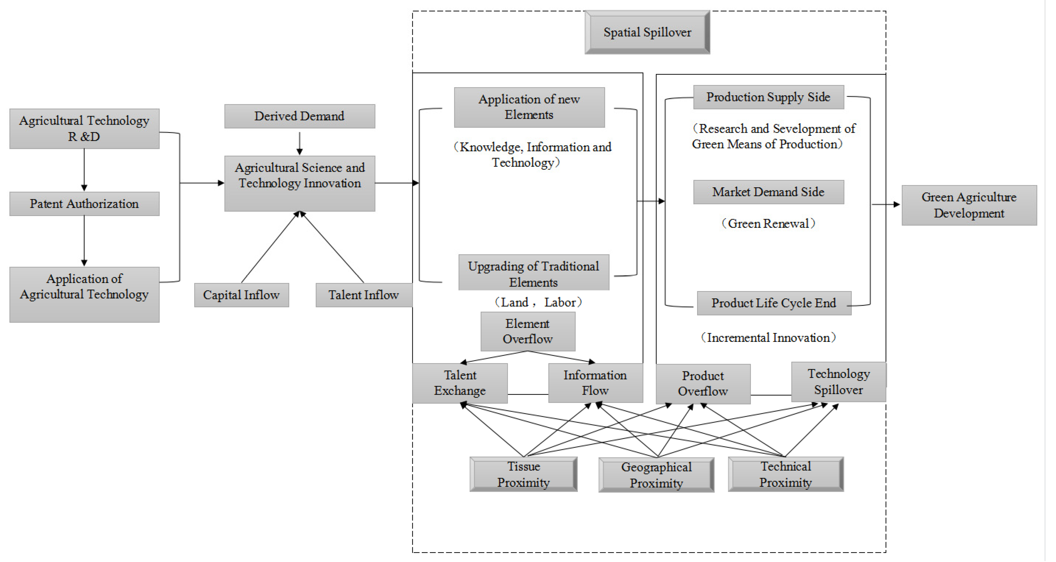
2. Influence Mechanism

Based on the perspective of spatial spillover, scientific and technological agricultural innovation is an important way to improve the level of agricultural green development. This is because the interregional flow of factors and products will promote the optimal allocation of resources in space, accelerate the dissemination and diffusion of innovative technology, knowledge, experience and information through the spatial spillover effect, strengthen the basic conditions of local innovation activities and promote the local green development of agriculture. Accordingly, in this paper, we divide the spatial spillover path of scientific and technological agricultural innovation on agricultural green development into the factor spillover path and the product spillover path, and we reveal the impact mechanism of scientific and technological agricultural innovation on green agricultural development (Figure 1).

From the perspective of the factor path, scientific and technological agricultural innovation itself is the result of the interaction and synergy of relevant factors, such as science, technology and organization. Through the two stages of agricultural technology, namely, R&D and agricultural technology application, scientific and technological agricultural innovation will promote the application of new factors, such as the efficient use of new capital elements through financial investment, talent introduction and learning demonstrations. Information elements and technical elements will also lead to the further upgrading of traditional elements, such as the upgrading of labor elements through talent training. Combined with economic externality theory and proximity dynamics theory, scientific and technological agricultural innovation is characterized as a public good and has strong positive externalities. Based on the perspective of multidimensional proximity, talent, knowledge, information and other elements of scientific and technological agricultural innovation will flow between regions via geographical proximity, organizational proximity and technological proximity. In particular, regions with high geographical proximity have less spatial distance and low communication costs, which is conducive to the flow of elements between regions; regions with high organizational proximity can more effectively obtain the spillover of remote knowledge and technology under the same external business environment, and in regions with high technical proximity, a knowledge structure with high similarity will promote knowledge spillover. Therefore, there is a spatial spillover effect of scientific and technological agricultural innovation in adjacent regions. This can achieve the reuse and re-upgrading of factors through the spillover and flow of factors among regions so as to improve the development level of agricultural green development in adjacent regions.

Product spillover is also one of the important paths for scientific and technological agricultural innovation to improve the development level of green agriculture in adjacent regions through the spatial spillover effect. Under the joint action of new elements and traditional elements, scientific and technological agricultural innovation will promote agricultural green development through three aspects: the production supply end, market demand end and product life cycle end. Among these aspects, the production supply side mainly refers to the fact that scientific and technological agricultural innovation can carry out R&D and the implementation of green means of production, such as biological pesticides, biological fertilizers and organic fertilizers, and apply the products to green production in adjacent areas through product spillover so as to realize the dual improvement of local and adjacent regional economic benefits and speed up the process of agricultural green production. The market demand side mainly refers to the fact that scientific and technological agricultural innovation can update the products of traditional agricultural production by integrating resource advantages so as to enrich the product diversity of local and adjacent regions and expand the market demand through product spillover. The product life cycle aspect mainly refers to the fact that scientific and technological agricultural innovation can gradually improve products, prolong the life cycle of green agricultural products, carry out technological innovation on the performance and quality of agricultural products to increase product demand at the stage of rising product demand and carry out gradual innovation on original products during product recession. The updated green agricultural products flow between adjacent areas so as to improve their market adaptability.

3. Research Model Design

3.1. Measurement of China’s Agricultural Green Development Level

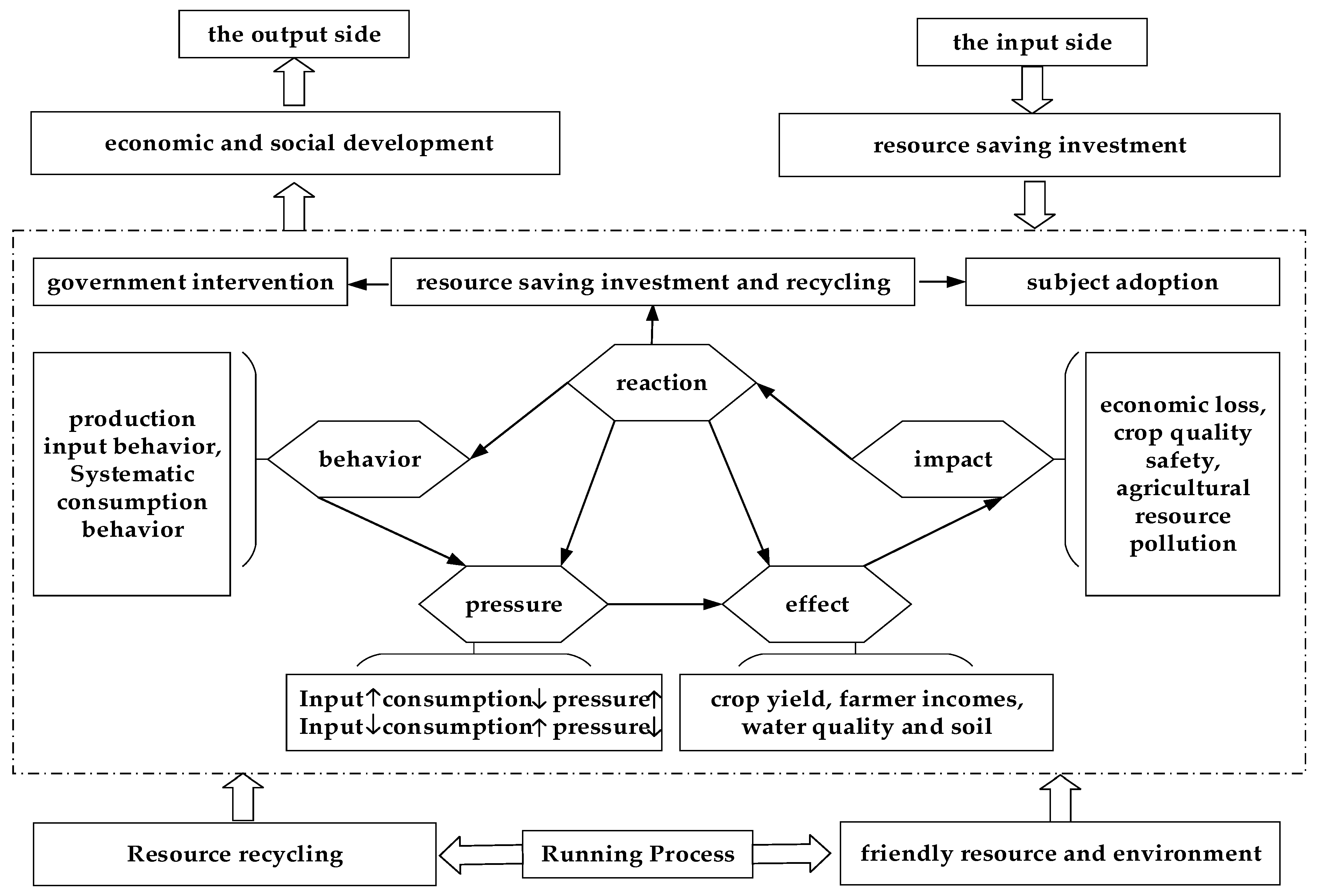
3.1.1. Construction of BPEIR Conceptual Model

Vigorously developing the agricultural circular economy is an effective way to achieve sustainable agricultural development and is a strategic measure to relieve pressure on agricultural resources, protect ecology, use clean resources and promote green agricultural development and sustainable rural economic development. This paper is based on the theory of the agricultural circular economy and comprehensively evaluates the development level of agricultural green development by constructing the BPEIR conceptual model. The BPEIR conceptual model, namely, the “behavior–pressure–effect–impact–response” model (Figure 2), is one of the typical quantitative models of the agricultural circular economy. The model assumes that the green agricultural production system consists of several regional systems and that there is total circulation in the system, whose size is determined by its external input and internal consumption. Specifically, if the use of system resources in a region increases and the consumption decreases, this behavior will increase the pressure on the system, resulting in negative effects. For example, in agricultural production, the abuse of fertilizers and pesticides will reduce the actual effective utilization rate and then lead to a reduction in crop yield and a decline in farmers’ income. The accumulation of negative effects has a strong impact on the system, causing economic and ecological problems, which forces the main body to respond to them and take a series of measures that are conducive to agricultural production to reduce the pressure on the system, such as controlling the total amount of agricultural water use. Additionally, environmentally polluted agricultural water, the reduced use of chemical fertilizers and pesticides, livestock and poultry manure, agricultural film and crop straw are resourced, comprehensively recycled and reused as harmless treatment measures to achieve resource-saving input and resource recycling. On the contrary, if resource usage in a regional system decreases, consumption increases and resource recycling is realized, decreasing the system pressure, which is conducive to benign development. In conclusion, based on the BPEIR conceptual model, this paper comprehensively evaluates the development level of green agriculture by considering the input, process and output of the system.

3.1.2. Construction of an Indicator System for Measuring the Development Level of Green Agriculture

At present, there is no unified and complete evaluation system for the measurement of the development level of green agriculture. This article is based on the BPEIR conceptual model combined with the Green Development Index System issued by the Ministry of Environmental Protection and the National Development and Reform Commission and the basic guidelines of Made in China 2025. The evaluation of agricultural green development should fully consider social, economic and ecological benefits to accurately and truly reflect the important content involved in the input, output and operation of the green agricultural production system. Considering the science and availability of data, in this article, we propose a green agricultural development level measurement index system with 18 indicators in 4 dimensions: economic and social development, resource-saving investment, resource recycling and resource and environmental friendliness. The specific measurement index system is shown in

Table 1. Indicator system for measuring the development level of green agriculture.

First-Level Indicators	Secondary Indicators	Unit of Measurement	Indicator Type	Interpretation of Indicators
Economic and social development	Agricultural GDP output value per unit area	CNY/hm2	Positive	Agricultural GDP output value/sown area of crops
	Per capita disposable net income of farmers	CNY/person	Positive	Farmers’ total income per capita minus various expenditures per farmer
	Per capita grain production	kg/person	Positive	Total food production/total population
	Per unit area yield of grain	kg/hm2	Positive	Food production/area of arable land
	Total power of agricultural machinery	Ten thousand kW	Positive	Agricultural machinery power + forestry machinery power + animal husbandry and fishery machinery power
Resource-saving investment	Fertilizer application intensity	kg/hm2	Negative	Scalar amount of fertilizer application/sown area of crops
	Intensity of pesticide use	kg/hm2	Negative	Pesticide use/sown area of crops
	Intensity of agricultural mulch use	kg/hm2	Negative	Amount of agricultural film used/sown area of crops
	Intensity of agricultural water use	m3/hm2	Negative	Total water consumption/sown area of crops
Resource recycling	Coefficient of effective use of chemical fertilizer	CNY/kg	Positive	Planting industry output value/scalar amount of chemical fertilizer application
	Effective utilization coefficient of pesticide	CNY/kg	Positive	Planting industry output value/amount of pesticide use
	Water-saving irrigation coefficient	%	Positive	Water-saving irrigation area/total irrigation area × 100%
	Cultivated land multiple cropping index	%	Positive	Sown area of crops/area of arable land × 100%
Resource environmental friendliness	Total agricultural chemical oxygen demand COD emissions	Ten thousand tons	Negative	Agricultural waste discharge
	Total agricultural ammonia nitrogen emissions	Ten thousand tons	Negative	Agricultural waste discharge
	Forest cover rate	%	Positive	Forest area/total land area × 100%
	Annual afforestation area	hm2	Positive	Annual afforestation area
	Proportion of area of nature reserves	%	Positive	Area of natural resource protection area/area of jurisdiction × 100%

.

3.1.3. Inspection of the Indicator System for Measuring the Development Level of Agricultural Green

(1) Single-element inspection

Single-unit testing is used to analyze individual indicators from the perspective of operability, accuracy and authenticity so as to ensure that the obtained indicator data are true and reliable. First, for the available data, the data sources were selected from the China Agricultural Yearbook, China Statistical Yearbook, China Forestry Statistical Yearbook, China Environmental Yearbook and China Water Conservancy Statistical Yearbook. Second, in addition to the existing statistical yearbook data, there were still a few indicators that needed to be measured. The specific indicators are explained in Table 1. Finally, during data collection, some provinces were found to have missing data for certain indicators. In this case, calculation methods such as linear interpolation and the mean filling method were selected to ensure the integrity of the agricultural green measurement indicator data.

(2) Overall inspection of elements

The overall inspection of the agricultural green development level measurement index system mainly starts with the specific inspection from three aspects: consistency, completeness and necessity. Specifically, consistency measures the consistency of the range of the index calculation and the calculation method. The completeness of the indicators reflects the input end, output end and the important content involved in the operation process of the green agricultural production system. Necessity tests the irreplaceability of each index element from the perspective of the whole index system. This paper focuses on the overall necessity of eliminating indicators that are not representative or highly correlated by calculating identification and redundancy. In particular, the recognition degree is calculated by the minimum mean square error method, and the formula is as follows:

$$S_j=\sqrt{\frac{1}{n}{\displaystyle \sum _{i=1}^n{(x_{ij}-{\overline{x}}_j)}^2}},j=1,2,3,\cdots m$$

(1)

In the formula, $S_j$ is the evaluation object, and $x_{ij}$ is the jth index value of the ith evaluated object. If $k_0(1\le k_0\le m)$ exists, then $S_{k_0}=\underset{1\le j\le m}{\min }\{S_j\}$. Then, the evaluation index $x_{k_0}$ corresponding to $S_{k_0}$ can be eliminated.

It can be seen from

Table 2. Recognition degree results.

Index	Standard Deviation	Index	Standard Deviation
Agricultural GDP output value per unit area	24,911.86	Coefficient of effective utilization of chemical fertilizer	46.17
Per capita disposable net income of farmers	5250.80	Coefficient of pesticide effective utilization	3761.49
Per capita food production	334.74	Coefficient of water-saving irrigation	22.72
Grain yield	1709.29	Cultivated land multiple cropping index	38.30
Total power of agricultural machinery	3124.55	Total agricultural chemical oxygen demand COD emissions	34.08
Fertilizer application intensity	129.17	Total agricultural ammonia nitrogen emissions	2.05
Intensity of pesticide use	9.35	Forest cover rate	17.67
Intensity of agricultural mulch use	14.36	Annual afforestation area	156,693.30
Intensity of agricultural water use	14,644.74	Proportion of area of nature reserves	5.85

that the standard deviation calculated for the total agricultural ammonia nitrogen emission index is 2.05, which is the smallest standard deviation among all indicators, indicating that this indicator is not representative. Although it can indicate the degree of resource and environmental friendliness in theoretical analysis, the scores of green agricultural development in China’s 30 provinces from 2006 to 2019 are comparable for this indicator; that is, the impact of this indicator on the ranking of units is negligible, so it can be eliminated.

Proceeding from the four first-level indicators of economic and social development, resource-saving investment, resource recycling and resource and environmental friendliness, the irreplaceability of various indicators is ensured by performing a layered measurement of redundancy. The principle is to select independent indicators with very little correlation with other indicators. The specific steps are as follows:

Step 1: Calculate the correlation coefficient matrix $R=(r_{ij}),r_{ij}=\frac{S_{ij}}{\sqrt{S_{ii}·S_{jj}}},i,j=1,2,\cdots ,m$. Here, $S_{ij}(i\ne j)$ is the covariance, and $S_{ii}$ and $S_{jj}$ are the variance.

Step 2: Calculate the correlation degree between the ith index and the other m−1 indexes in each layer; that is, the multiple correlation coefficient, which is defined as ${\delta }_i$. Replace the ith row and jth column of matrix R to the last row and last column of the matrix at the time $R\to \left[\begin{array}{cc}{R}_{-i}& r_i\\ r_i^T& 1\end{array}\right]$; then, the calculation formula of the multiple correlation coefficient is:

$${\delta }_i=r_i^T·R_{-i}^{-1}·r_i,i=1,2,\cdots ,m$$

(2)

Step 3: After calculating ${\delta }_1,{\delta }_2,\cdots ,{\delta }_m$, determine which indicator has the largest value: this indicator has the highest correlation with the other indicators in the layer and is easy to replace. Specify the lower limit of the critical value D when ${\delta }_i>D$; then, this indicator can be eliminated.

Step 4: Repeat the above steps until ${\delta }_i\le D$ is reached.

As can be seen from

Table 3. The redundancy results of the index calculated by the “maximum uncorrelation method”.

First-Level Indicators	Secondary Indicators	Multiple Correlation Coefficient
Economic and social development	Agricultural GDP output value per unit area	0.682
	Per capita disposable net income of farmers	0.661
	Per capita grain production	0.569
	Per unit area yield of grain	0.708
	Total power of agricultural machinery	0.676
Resource-saving investment	Fertilizer application intensity	0.610
	Intensity of pesticide use	0.614
	Intensity of agricultural mulch use	0.458
	Intensity of agricultural water use	0.181
Resource recycling	Coefficient of effective use of chemical fertilizer	0.278
	Effective utilization coefficient of pesticide	0.350
	Water-saving irrigation coefficient	0.601
	Cultivated land multiple cropping Index	0.587
Resource and environmental friendliness	Total agricultural chemical oxygen demand COD emissions	0.229
	Total agricultural ammonia nitrogen emissions	0.359
	Forest cover rate	0.234
	Annual afforestation area reserves	0.376

, for the economic and social development index, the critical lower limit D is 0.70. Since the complex correlation coefficient between the grain yield per unit area and other indexes within the layer exceeds 0.70, the grain yield per unit area index is eliminated. For the resource-saving input index, resource recycling index and resource and environment friendliness index, the complex correlation coefficient ${\delta }_i\le D$ indicates that these indexes are not highly correlated with each other, so they are retained. Through the single test and overall test of the green agricultural development level index system, two indexes—total agricultural ammonia nitrogen emission and grain yield per unit area—were eliminated on this basis, and finally, an evaluation index system of agricultural green development was formed, which included 4 first-level indexes and 16 specific indexes.

3.1.4. Construction of Agricultural Green Development Level Measurement Model

Gray correlation analysis is a method to measure the development trend of the gray system. Its basic principle is to infer whether there is an influence between the factors and the degree of influence based on the similarity of the curve shape of the behavior factor series. If the curve shape similarity between the comparison series and the reference series is high, it indicates that the relationship between the two series is relatively close, and the gray correlation degree between the two series is relatively large; on the contrary, it indicates that the gray correlation degree between the two series is small. The specific steps are as follows.

Step 1: Determine the comparison sequence. Based on the measured value of each indicator in the green agricultural development level measurement indicator system, the comparison series is as follows:

$$X_{ij}=\left[\begin{array}{cccc}{X}_{11}& X_{12}& \cdots & X_{1n}\\ X_{21}& X_{22}& \cdots & X_{2n}\\ ⋮& ⋮& ⋮& ⋮\\ X_{m1}& X_{m2}& \cdots & X_{mn}\end{array}\right]$$

(3)

Step 2: Standardize each indicator. Since the measurement units of the existing initial data are not uniform, and there is a difference between positive and negative indicators, it is necessary to normalize the selected initial data to obtain a dimensionless matrix:

$$Y_{ij}=\left[\begin{array}{cccc}{Y}_{11}& Y_{12}& \cdots & Y_{1n}\\ Y_{21}& Y_{22}& \cdots & Y_{2n}\\ ⋮& ⋮& ⋮& ⋮\\ Y_{m1}& Y_{m2}& \cdots & Y_{mn}\end{array}\right]$$

(4)

Step 3: Determine the reference sequence and calculate the difference sequence. The reference sequence is usually composed of the optimal value of each comparison sequence. For a sample containing m research objects and n indicators, the reference sequence is usually expressed as $Y_o=\{Y_{o1},Y_{o2},\cdots ,Y_{on}\}$.

Step 4: Find the gray correlation coefficient. Correlation is the degree of difference in geometric shapes between curves. Calculate the gray correlation coefficient between the jth index of the ith province and the reference series. The formula is as follows:

$${\epsilon }_{ij}=\frac{\underset{i}{\min }\underset{j}{\min }\left|Y_{ij}-Y_{oj}\right|+\rho \underset{i}{\max }\underset{j}{\max }\left|Y_{ij}-Y_{oj}\right|}{\left|Y_{ij}-Y_{oj}\right|+\rho \underset{i}{\max }\underset{j}{\max }\left|Y_{ij}-Y_{oj}\right|}$$

(5)

In the formula, $\rho$ is the resolution coefficient and $0\le \rho \le 1$, which plays a role in increasing the significance of the correlation coefficient difference, usually taken as $\rho =0.5$.

Step 5: Find and sort the degree of gray correlation. This paper uses the absolute value correlation method to calculate the correlation coefficient of each evaluation subject of the agricultural green development level. The greater the correlation, the higher the similarity. The closer the comparison series is to the reference series, the better the agricultural green development level measurement index, and vice versa. The formula is as follows:

$${\gamma }_i=\frac{1}{n}{\displaystyle \sum _{j=1}^n{\epsilon }_{ij}}$$

(6)

In the formula, ${\gamma }_{\mathrm{i}}$ is the ith gray correlation degree, ${\epsilon }_{\mathrm{ij}}$ is the ith gray correlation coefficient, and n is the number of ${\epsilon }_{\mathrm{ij}}$.

3.2. Measurement of Spatial Spillover of Agricultural Technological Innovation on the Level of Agricultural Green Development

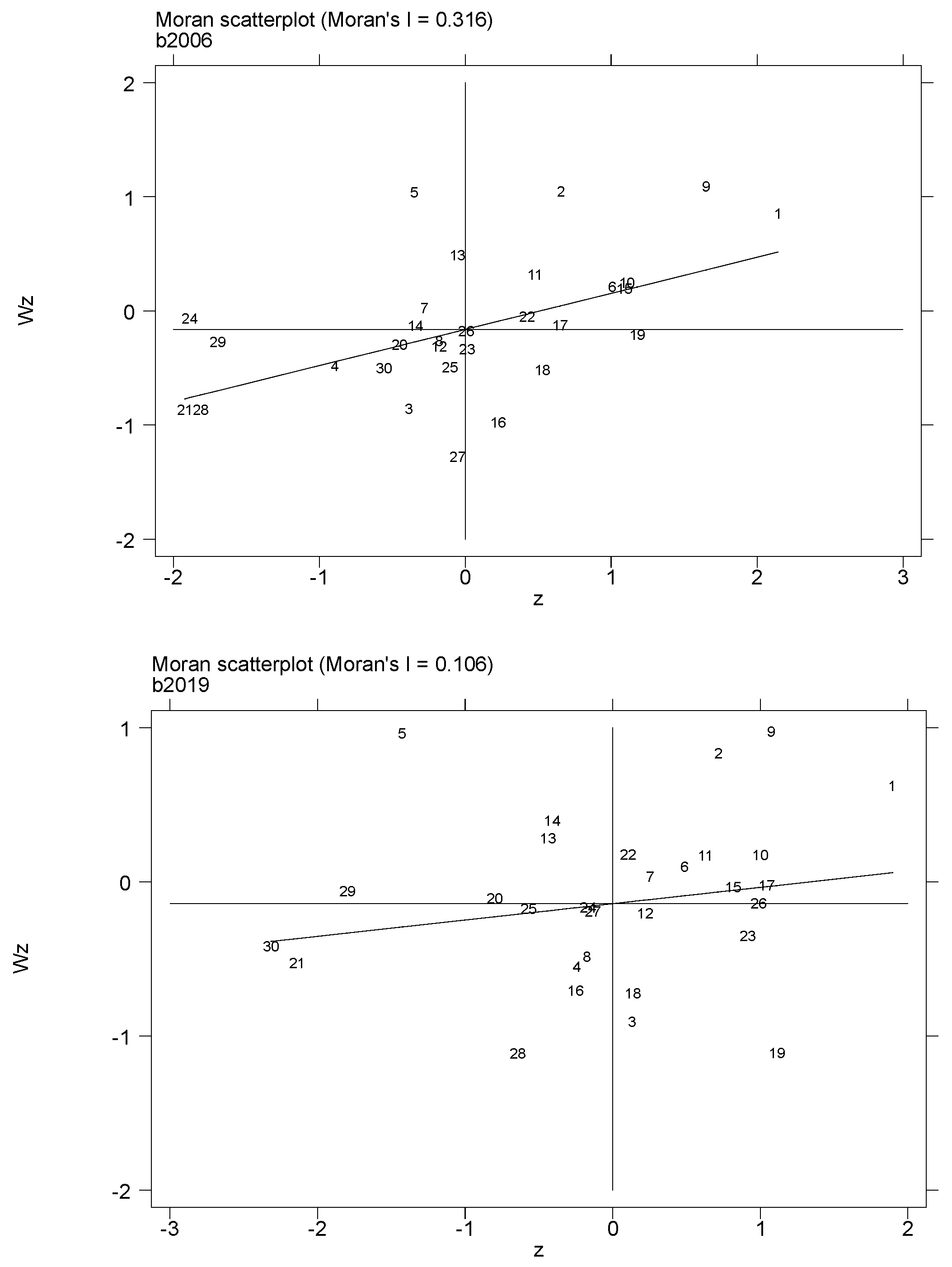
3.2.1. Spatial Autocorrelation Test

(1) Global spatial autocorrelation

Global spatial autocorrelation is an index that measures the spatial correlation of research objects from a global perspective. This article uses the global Moran’s index to measure the global spatial pattern of agricultural technological innovation and green agricultural development, and its value range is [−1,1], with 0 as the dividing line. When the value is greater than 0, this indicates that the variable has a positive spatial correlation—that is, spatial agglomeration; when the value is less than 0, it indicates that the variable has a negative spatial correlation—that is, spatial dispersion; when the value is equal to 0, it indicates that the variables are not spatially correlated and are randomly distributed.

$$Moran’sI=\frac{n{\displaystyle \sum _{i=1}^n{\displaystyle \sum _{j=1}^n{W}_{ij}(X_i-\overline{X})(X_j-\overline{X})}}}{{\displaystyle \sum _{i=1}^n{(X_i-\overline{X})}^2{\displaystyle \sum _{i=1}^n{\displaystyle \sum _{j=1}^{n}Wij}}}}=\frac{{\displaystyle \sum _{i=1}^n{\displaystyle \sum _{j=1}^n{W}_{ij}(X_i-\overline{X})(X_j-\overline{X})}}}{S^2{\displaystyle \sum _{i=1}^n{\displaystyle \sum _{j=1}^{n}Wij}}}$$

(7)

Here, $S^2=\frac{{\displaystyle \sum _{i=1}^n{(X_i-\overline{X})}^2}}{n}$ is the variance of the observation unit, n is the number of observation units, $W_{ij}$ is the spatial weight matrix, and $X_i$ and $X_j$ are the values of variable X on spatial units i and j.

(2) Local spatial autocorrelation

Local spatial autocorrelation is an index to measure the spatial correlation of research objects from a local perspective. In this paper, Moran’s index is used to identify the local spatial pattern characteristics of agricultural science and technology innovation and agricultural green development, which can be divided into four types of agglomeration. The first type is high-value agglomeration (HH), which indicates that the innovation level of agricultural science and technology in the province is high, and that of the neighboring provinces is also high, presenting a high-level mean spatial correlation agglomeration state of “high in the center, high in the surrounding areas”. The second type is low-value collapse (LH), which indicates that the innovation level of agricultural science and technology in the province is low, but the innovation level of agricultural science and technology in the neighboring provinces is high, presenting a spatial disequilibrium correlation agglomeration state of “low in the center, high in the surrounding areas”. The third type is low-value agglomeration (LL), which indicates that the innovation level of agricultural science and technology in this province is low, and that of its neighboring provinces is also low, presenting a low-level mean spatial correlation agglomeration state of “low in the center, low in the surrounding areas”. The fourth type is high-value bulge (HL), which indicates that the agricultural science and technology innovation level of the province is high, but that of the neighboring provinces is low, presenting a spatial disequilibrium correlation agglomeration state of “high in the center, low in the surrounding areas”. The specific calculation formula of the local Moran’s index is as follows:

$$Moran’s{I}_i=\frac{n(X_i-\overline{X}){\displaystyle \sum _{j=1}^n{W}_{ij}(X_j-\overline{X})}}{{\displaystyle \sum _{i=1}^n{(X_i-\overline{X})}^2}}=\frac{(X_i-\overline{X}){\displaystyle \sum _{j=1}^n{W}_{ij}(X_j-\overline{X})}}{S^2}$$

(8)

3.2.2. Spatial Measurement Model

(1) Spatial panel measurement model setting

Spatial panel measurement models are classified into different categories due to the similarities and differences between the lag and error terms, and they mainly include three types: spatial lag model (SLM), spatial error model (SEM) and spatial Dubin model (SDM). The expressions of the three spatial panel measurement models constructed in this paper are as follows:

Spatial lag model (SLM):

$$Y=\rho wY+\beta X+\epsilon ,\epsilon ~N(0,{\sigma }^2{I}_n)$$

(9)

Spatial error model (SEM):

$$Y=\beta X+\mu ,\mu =\lambda w\mu +\epsilon ,\epsilon ~N(0,{\sigma }^2{I}_n)$$

(10)

Spatial Dubin model (SDM):

$$Y=\rho wY+\beta X+\varsigma wX+\epsilon ,\epsilon ~N(0,{\sigma }^2{I}_n)$$

(11)

Spatial effect decomposition (partial differential equation):

$$Y={(1-\rho w)}^{-1}n{i}_n+{(1-\rho w)}^{-1}(\beta X+\varsigma wX)+{(1-\rho w)}^{-1}\epsilon$$

(12)

$$\left(\frac{\partial Y}{\partial X_{1k}}\frac{\partial Y}{\partial X_{2k}}\cdots \frac{\partial Y}{\partial X_{nk}}\right)=\left(\begin{array}{cccc}\frac{\partial Y_1}{\partial X_{1k}}& \frac{\partial Y_1}{\partial X_{2k}}& \cdots & \frac{\partial Y_1}{\partial X_{nk}}\\ \frac{\partial Y_2}{\partial X_{1k}}& \frac{\partial Y_2}{\partial X_{2k}}& \cdots & \frac{\partial Y_2}{\partial X_{nk}}\\ ⋮& ⋮& \ddots & ⋮\\ \frac{\partial Y_n}{\partial X_{1k}}& \frac{\partial Y_n}{\partial X_{2k}}& \cdots & \frac{\partial Y_n}{\partial X_{nk}}\end{array}\right)={(1-\rho w)}^{-1}\left(\begin{array}{cccc}{\beta }_k& w_{12}{\varsigma }_k& \cdots & w_{1n}{\varsigma }_k\\ w_{21}{\varsigma }_k& {\beta }_k& \cdots & w_{2n}{\varsigma }_k\\ ⋮& ⋮& \ddots & ⋮\\ w_{n1}{\varsigma }_k& w_{n2}{\varsigma }_k& \cdots & {\beta }_k\end{array}\right)$$

(13)

In the formulas, $Y$ is the explained variable (agricultural green development level), $X_{ik}$ is the Kth explanatory variable, $w$ is the spatial weight matrix, $\rho$ is the spatial autoregression coefficient of the explained variable, $\lambda$ is the spatial regression coefficient of the error term, ${\varsigma }_{1-6}$ is the spatial regression coefficient of the error term, ${\beta }_{1-6}$ is the spatial regression coefficient of the explanatory variable, $\alpha$ is the constant term, and $\epsilon$ is the random error term. In partial differential equations, the mean value of each element on the diagonal of the matrix on the right side of the equation represents the direct effect of the kth explanatory variable $X_{ik}$, while the mean value $\frac{1}{n^2}{\displaystyle \sum _{i=1}^n{\displaystyle \sum _{j=1}^n{w}_{ij}{\varsigma }_k}}$ of other elements not on the diagonal is an indirect effect.

In addition, when $\varsigma =0,\rho \ne 0$, the SDM model will degenerate into SLM; when $\varsigma +\rho \beta =0$, the SDM model will degenerate into SEM.

(2) Construction of spatial weight matrix

The spatial weight matrix can reflect the correlation degree between spatial units, and it is very important to select it appropriately for the study of the spatial spillover effect between agricultural science and technology innovation and agricultural green development. Since agricultural science and technology innovation activities will inevitably be affected by a variety of other nongeographical proximity factors, and since there is a spatial correlation between the economic development levels of various provinces, science and technology innovation activities in underdeveloped provinces have little impact on developed provinces, while scientific and technological innovation activities of developed provinces have a great impact on the space of neighboring provinces. Therefore, this article adopts the spatial economic matrix (hereinafter referred to as the “economic matrix”) for quantification. The setting formula is:

$$W_{ij}=\{\begin{array}{l}\frac{1}{\left|{\overline{Y}}_i-{\overline{Y}}_j\right|},i\ne j,{\overline{Y}}_i=\frac{1}{t_1-t_0+1}{\displaystyle \sum _{t=t_0}^{t_1}{Y}_{it}}\\ 0,i=j\end{array}$$

(14)

3.3. Variable Selection and Data Sources

3.3.1. Variable Selection

The explained variable in this article is the level of agricultural green development, which is calculated using the gray correlation method. The core explanatory variable of this article is agricultural science and technology innovation. As far as its process is concerned, agricultural science and technology innovation is the result of the interaction and coordination among relevant elements, such as science, technology and organization. It progresses through basic research, applied research and the demonstration and extension of agricultural scientific research. Therefore, this article uses agricultural technology research and development and agricultural technology application to measure the level of agricultural technology innovation, specifically expressed as the number of agricultural patent authorizations and agricultural technology market turnover.

With reference to related research results, in this study, the following control variables were added: fiscal support for agriculture (FSA), expressed as the proportion of local financial expenditure on agriculture, forestry and water affairs in the sown area of crops (unit: yuan/hm²); agricultural machinery input intensity (MII), expressed as the proportion of the total power of agricultural machinery in the total sown area of crops (unit: kW/hm²); the agricultural disaster rate (ADR), expressed as the proportion of the affected area of crops in the total sown area of crops (unit: %); crop planting structure (CPS), expressed as the proportion of the planted area of food crops in the planted area of crops, excluding the planted area of food crops (unit: %); multiple cropping index (MCI), expressed as the proportion of the total planted area of crops in the cultivated area (unit: %).

3.3.2. Data Source

Based on the operability of the data, we selected panel data from 30 provinces (cities, districts) in China (excluding Tibet, Taiwan, Hong Kong and Macau) from 2006 to 2019 as the empirical research sample, with an observation value of 420. Except for agricultural patent data, basic data were obtained from the China Statistical Yearbook, China Fiscal Yearbook, China Rural Statistical Yearbook and the statistical yearbooks of various provinces and cities. The agricultural patent data were obtained from the patent database of the State Intellectual Property Office of China. The classification numbers representing agricultural patents were selected from the International Patent Classification System (IPC) to obtain relevant statistics on the number of agricultural invention patents and utility models granted. In order to eliminate problems such as heteroscedasticity in the regression process, logarithmic processing was performed on the relevant variables. The specific descriptive statistical results are shown in

Table 4. Variable description and descriptive statistical results.

Type	Variable	Variable Definition	Average	Standard Deviation	Minimum	Maximum
Explained variable	lnGad	Agricultural green development level value	3.8192	0.0724	3.6763	4.0270
Core explanatory variable	lnast	Number of agricultural patents granted	6.2525	1.2669	2.7726	8.8009
		Agricultural technology market turnover	13.3150	1.8573	8.5847	17.8577
		R&D personnel full-time equivalent	10.9618	1.2008	7.0975	13.5964
		Gross agricultural output value	6.9155	1.0493	3.6636	8.5957
Control variables	lnfsa	Financial expenditure on agriculture, forestry and water resources/sown area of crops	8.9747	1.0775	6.3045	13.4003
	lnmii	Total power of agricultural machinery/sown area of crops	1.7776	0.4325	0.7020	2.7314
	lnadr	Affected area of crops/sown area of crops	2.7010	0.8450	0.0032	4.2366
	lncps	Planting area of food crops/(planting area of crops minus planting area of food crops)	5.3392	0.7771	3.8228	8.1075
	lnmci	Sown area of crops/cultivated area	4.7764	0.3077	3.7543	5.3898

.

4. Analysis of Results

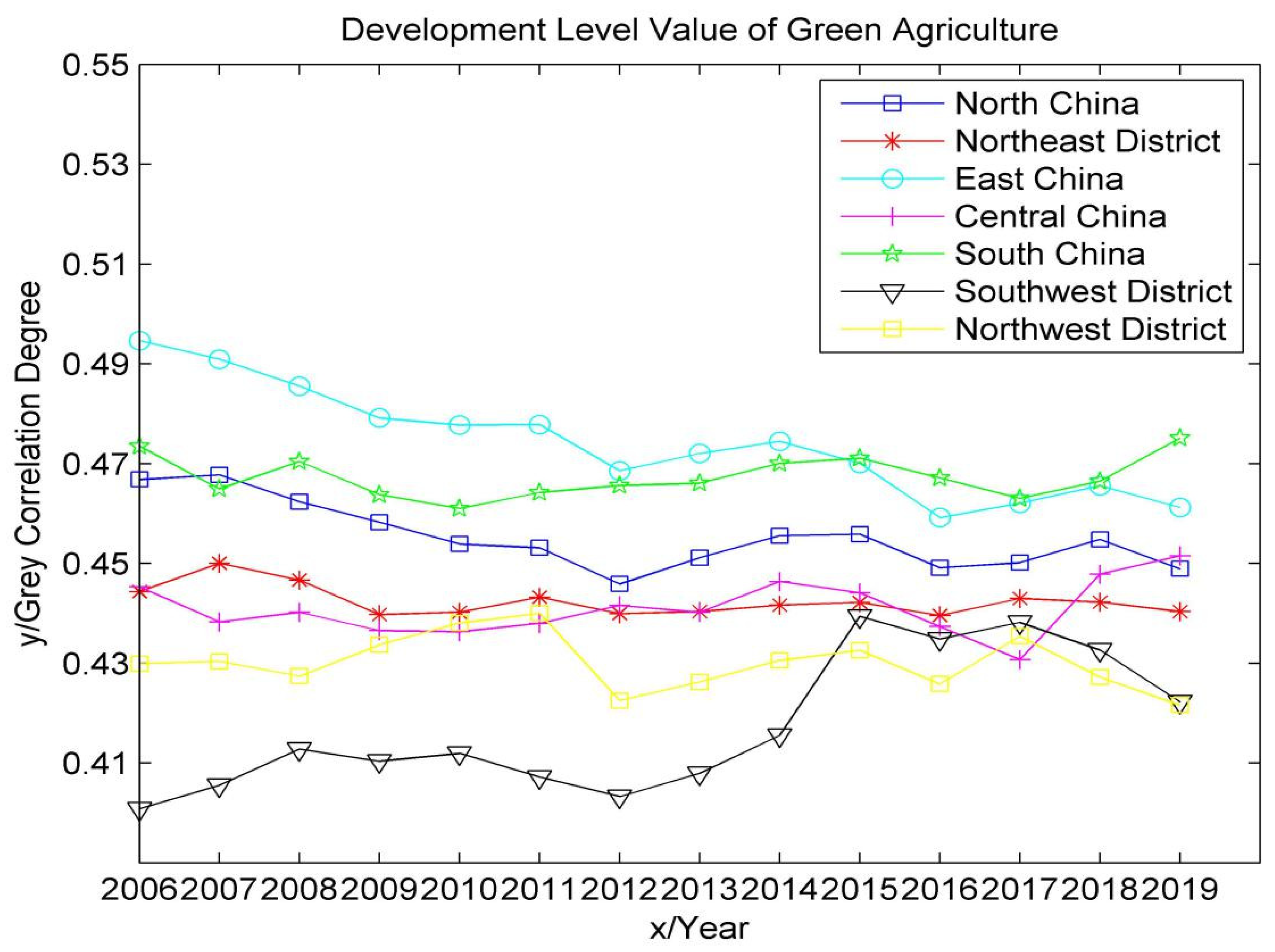
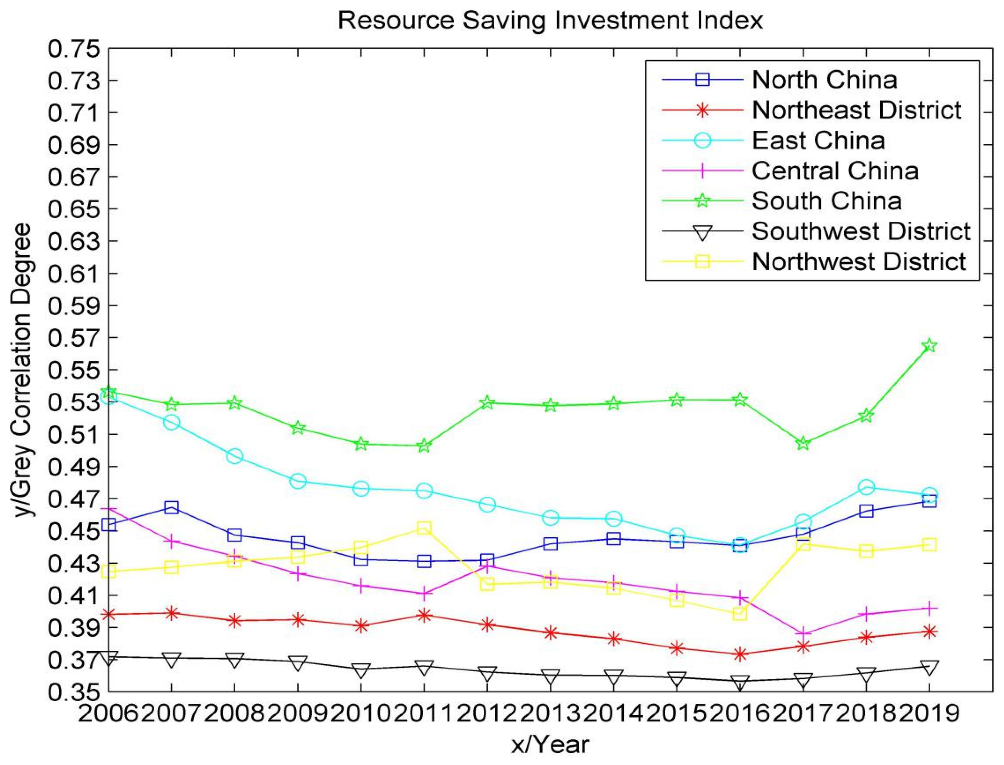
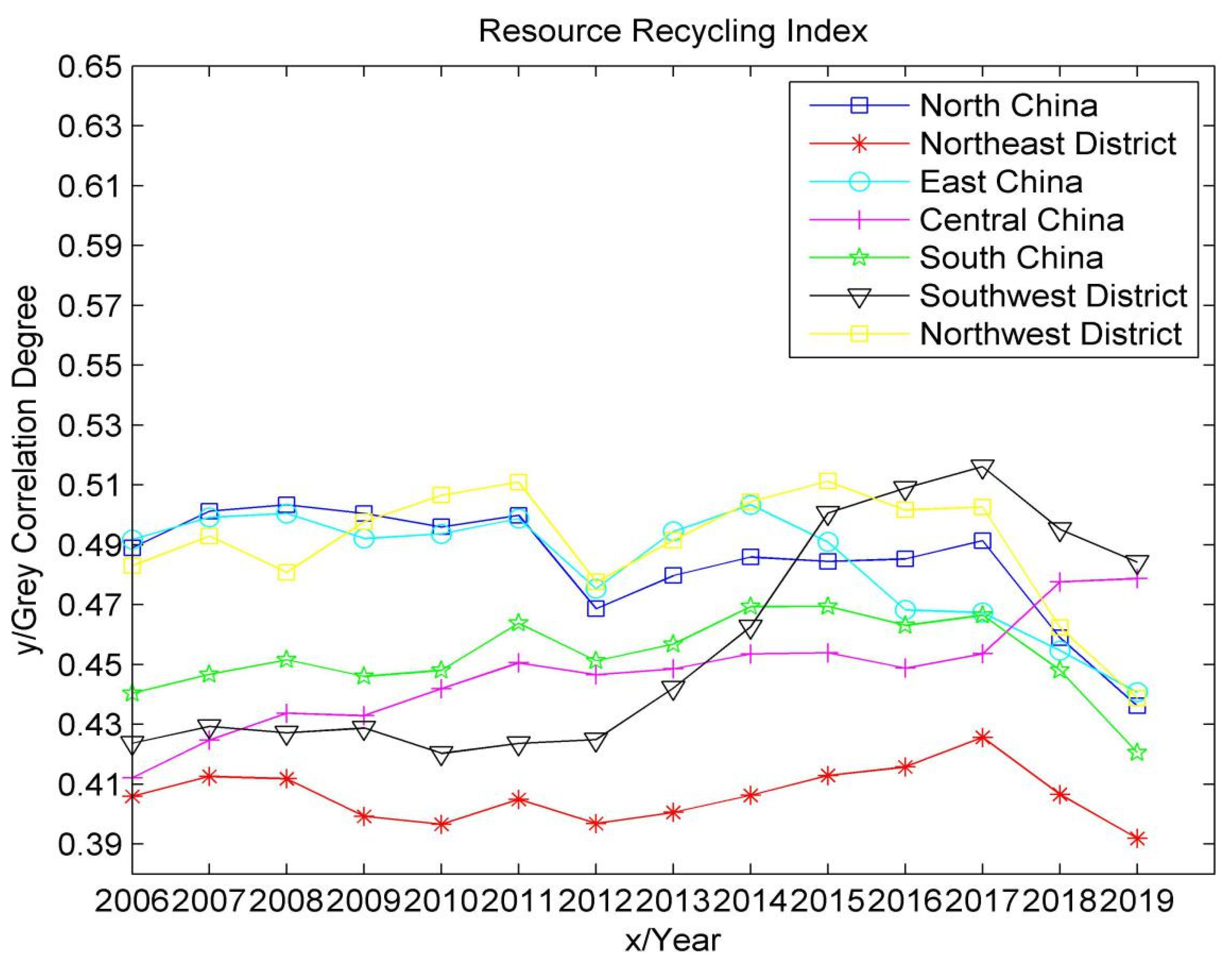
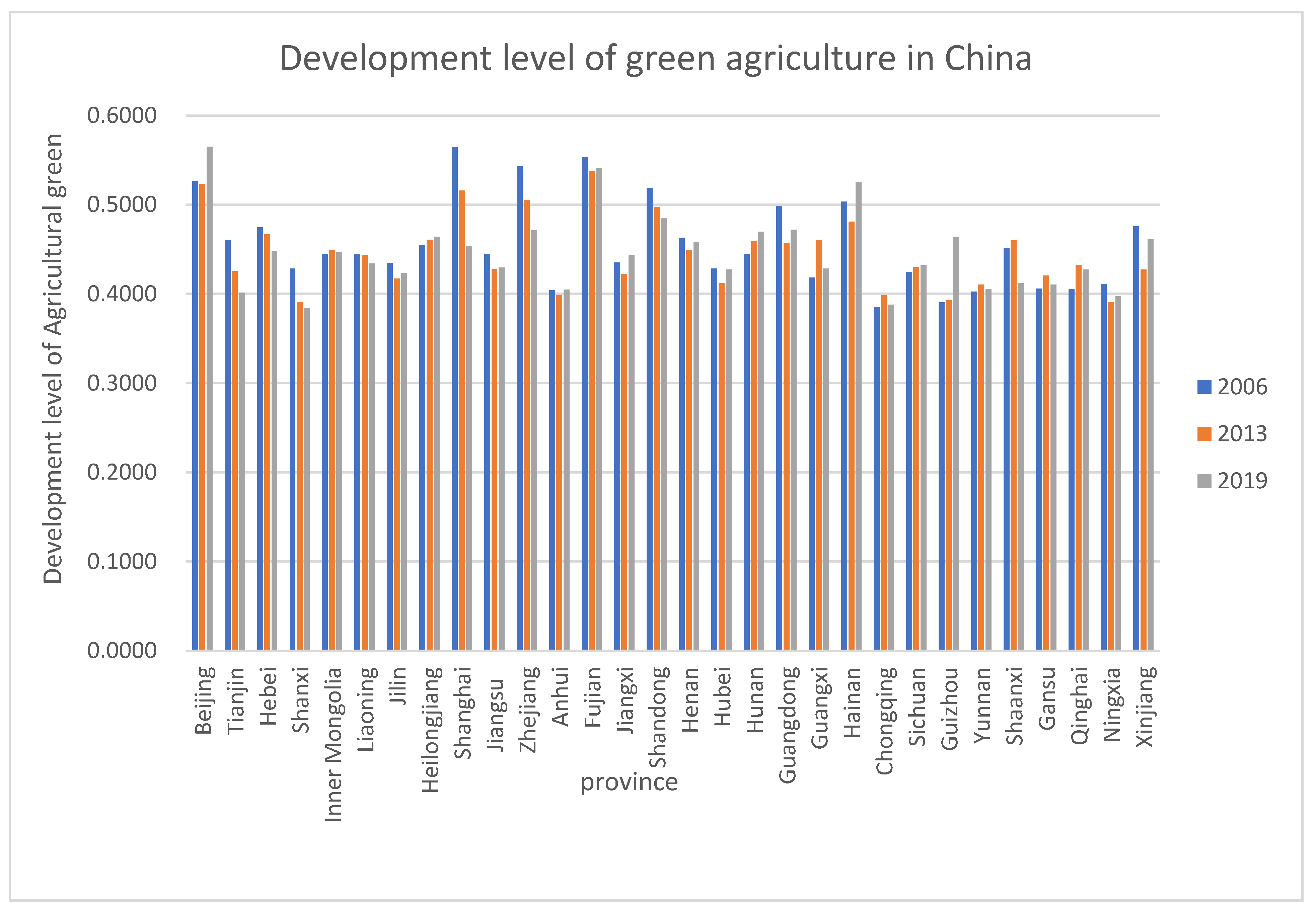
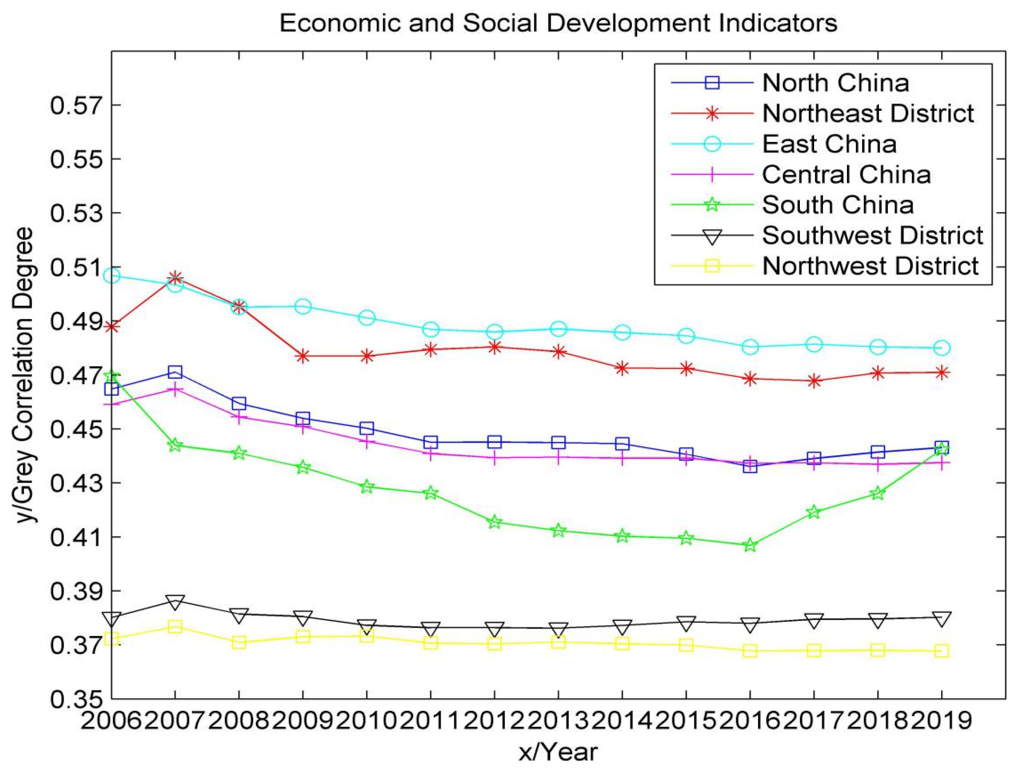
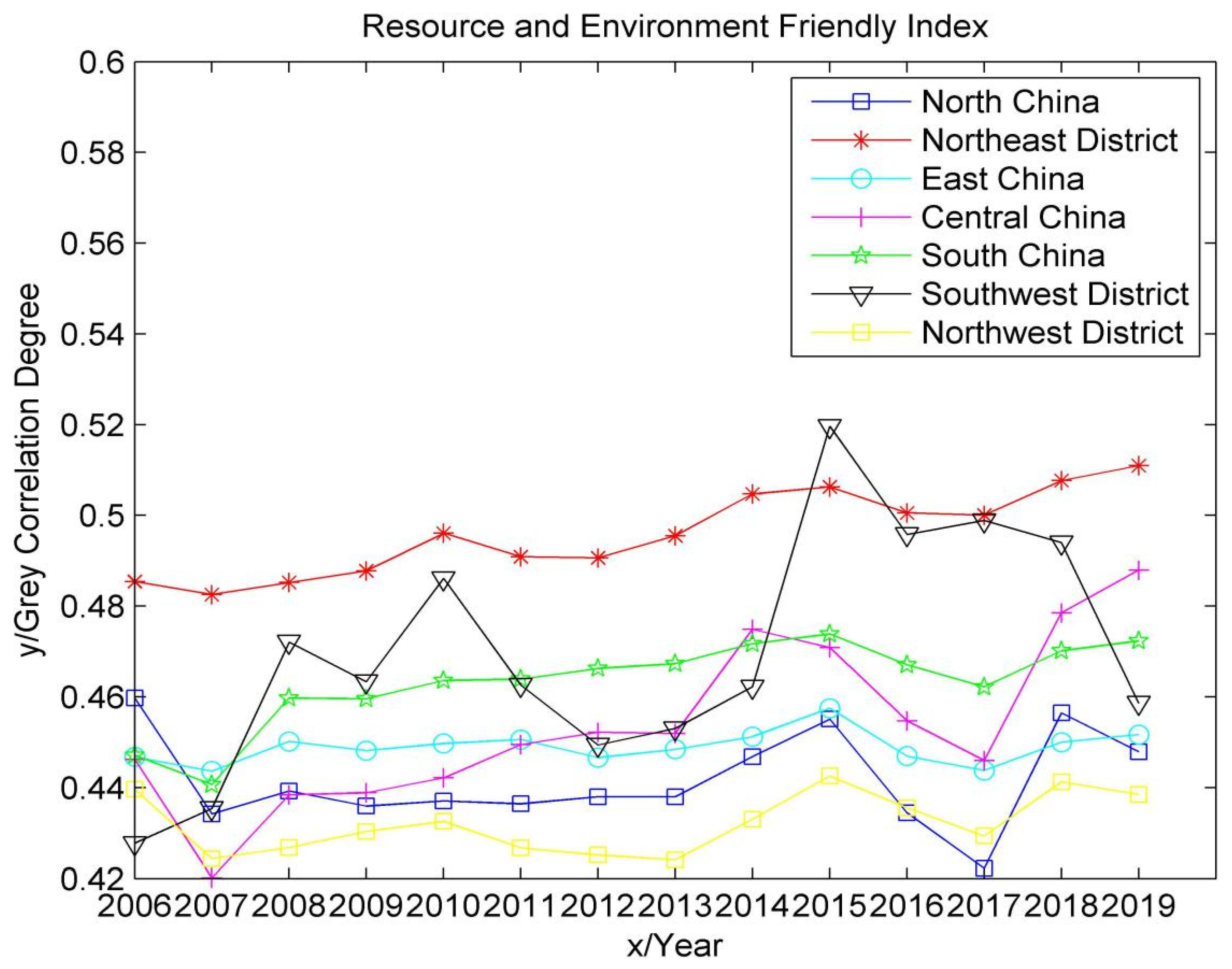
4.1. Analysis of the Results of Measurement and Spatial–Temporal Evolution of Agricultural Green Development Level

Dynamic Analysis of the Measurement Results of Agricultural Green Development Level

In this study, the gray correlation analysis method was used to calculate the level of agricultural green development in 30 provinces in China based on the data published in the China Statistical Yearbook from 2006 to 2019. Due to limited space, this paper only presents data from 2006, 2013 and 2019, as shown in Figure 3. Secondly, seven geographical regions of China, namely, north China, northeast China, east China, central China, south China, southwest China and northwest China (hereinafter referred to as the seven regions), were selected as the study regions. MATLAB software was used to analyze the temporal variation trend of the agricultural green development level evaluation index in the seven regions (excluding Tibet, Taiwan, Hong Kong and Macao) from four dimensions: economic and social development, resource-saving input, resource recycling and resource and environment friendliness, as shown in Figure 4, Figure 5, Figure 6, Figure 7 and Figure 8.

As can be seen from Figure 3, the agricultural green development level of 30 provinces in China was generally stable at 0.35–0.60. The average agricultural green development level of some provinces, such as Beijing and Fujian, is higher than 0.5, indicating a high agricultural green development level. The average value of the agricultural green development level in Shanxi and Chongqing is lower than 0.4, indicating that the development level of agricultural green in Shanxi and Chongqing is low. A possible reason is that Beijing and Fujian have a high level of economic and social development and have advanced crop management concepts, which have a positive role in promoting agricultural green development. However, Shanxi and Chongqing lack agricultural technology promotion and have insufficient agricultural industrialization infrastructure, and capital investment cannot introduce large-scale green development compound talent, which is not conducive to agricultural green development in central and western provinces and cities.

As can be seen from Figure 4, Figure 5, Figure 6, Figure 7 and Figure 8, the development level of green agriculture in east China and northwest China showed a fluctuating downward trend from 2006 to 2019, while southwest China showed a fluctuating upward trend. South China, north China, northeast China and Central China fluctuated between years, but the change was not large. Specifically, the highest level of agricultural green development is currently in east China, which has strong agricultural technological innovation capabilities and a high level of economic and social development. However, due to the fluctuating and decreasing trend of its resource-saving input indicators and resource recycling indicators, the overall value of the green agricultural development level shows a fluctuating downward trend. Among them, the resource-saving input indicators had a downward trend from 2006 to 2016, indicating that its fertilizers, pesticides, agricultural mulch film and agricultural water intensity were not effectively controlled, but it did rebound in 2016–2019, which may be due to the activeness of east China. Responding to important instructions on the insistence on green development, we must adhere to the basic national policy of saving resources and protecting the environment put forward by the Fifth Plenary Session of the 18th Central Committee, which strictly controls the intensity of the use of chemical fertilizers and pesticides to effectively improve resource utilization. The resource recycling index was relatively stable from 2006 to 2011, declined slightly in 2012 and increased from 2012 to 2014. This may be due to the proposal of the 18th National Congress of the Communist Party of China to “vigorously promote the construction of ecological civilization” in east China. The district began to focus on green development and circular development; the continuous decline from 2014 to 2019 was due to the rapid decline in the multiple cropping index during this period.

The lowest level of agricultural green development is in southwest China. Its agricultural technology innovation ability is weak, and its economic and social development level is low. However, due to the fluctuating and rising trend of its resource recycling index and resource/environmentally friendly index, the overall value of the agricultural green development level showed an upward trend in volatility. The index of resource recycling began to increase significantly in 2012, which may be due to the suggestion of “accelerating the construction of resource-conserving and environmentally friendly society and improving the level of ecological civilization” put forward in the 12th Five-Year Plan. The utilization rate of resources (fertilizer and pesticide) and water-saving irrigation coefficient in southwest China have been effectively improved. The decline in 2017 was caused by the rapid decline of the multiple cropping index. The resource/environmentally friendly index showed a fluctuating upward trend in 2006–2015, peaked in 2015, and declined in 2015–2019, mainly due to the large interannual fluctuations in the afforestation area. South China, north China, northeast China, central China and northwest China have an intermediate green agricultural development level, among which northwest China has the largest fluctuation and the lowest social development level. Additionally, because the fluctuation of the resource-saving input index is less than the fluctuation of the resource recycling index, the development level of green agriculture as a whole shows a small fluctuating downward trend. The index of resource-saving input started to decline in 2011, indicating that the resource factors of land input per hectare in northwest China were not reasonably controlled but rebounded in 2016. This may be due to the policy proposed by the Ministry of Agriculture in 2015, with the strategic goal of “one control, two reductions and three basics”, which stimulated the northwest district to begin to implement resource reduction strategies. The index of resource recycling increased from 2006 to 2011, decreased slightly in 2012, and increased from 2012 to 2015. This may be due to the active implementation of “strengthening the construction of ecological civilization system” proposed by the 18th National Congress of the Communist Party of China in 2012 in northwest China, which effectively improved the utilization rate of resources. The decrease from 2015 to 2019 is due to the decrease in the multiple cropping index during this period. The fluctuation is relatively gentle in south China, north China, northeast China and central China—especially in south China, where the resource-saving input index is always the highest, which may be due to the suggestion of “strengthening resource management” put forward in the “eleventh Five-Year Plan”, after which south China began to strengthen the protection and management of various natural resources.

4.2. Analysis of the Spatial Spillover Effect of Agricultural Science and Technology Innovation on Agricultural Green Development

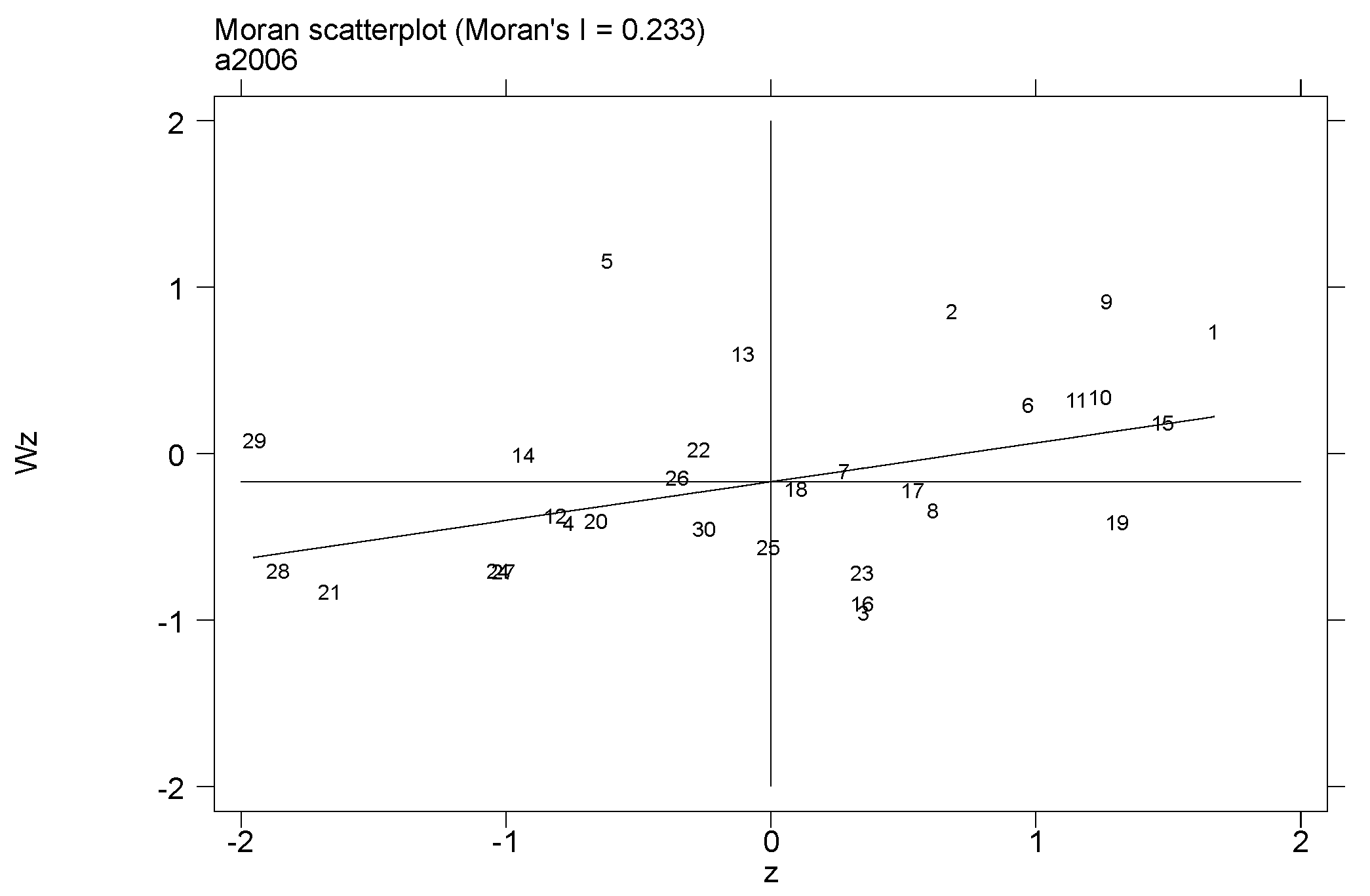
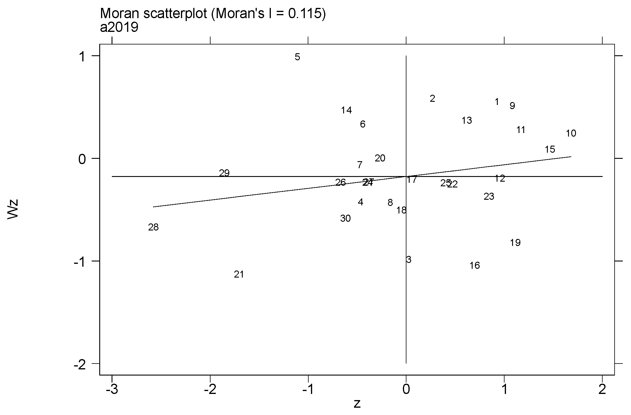
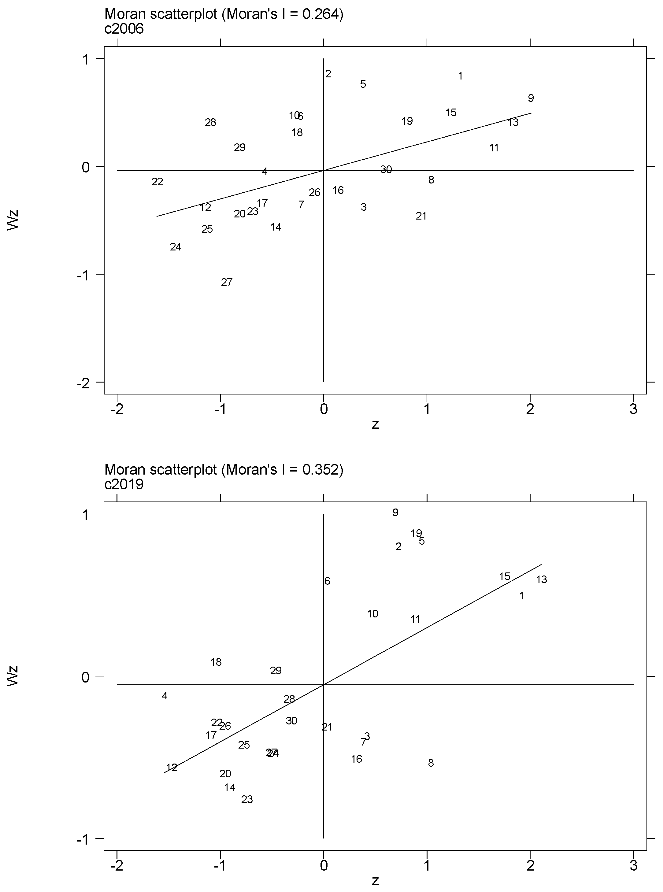
4.2.1. Spatial Autocorrelation Analysis of Agricultural Science and Technology Innovation and Agricultural Green Development

(1) Global spatial autocorrelation analysis

The overall Moran’s I index of agricultural science and technology innovation and the agricultural green development level from 2006 to 2019 was calculated using Equations (3)–(6), as shown in

Table 5. Moran’s I test results of global Moran’s index for agricultural technology development and agricultural technology application.

Years	Agricultural Technology R&D			Application of Agricultural Technology
	Moran’s I	Z Statistics	p-Value	Moran’s I	Z Statistics	p-Value
2006	0.233 ***	2.525	≤0.01	0.316 ***	3.354	≤0.01
2007	0.211 **	2.327	≤0.1	0.222 ***	2.466	≤0.01
2008	0.220 ***	2.408	≤0.01	0.215 ***	2.407	≤0.01
2009	0.173 **	1.968	≤0.05	0.221 ***	2.445	≤0.01
2010	0.192 **	2.147	≤0.05	0.243 ***	2.657	≤0.01
2011	0.163 **	1.893	≤0.05	0.307 ***	3.284	≤0.01
2012	0.147 **	1.747	≤0.05	0.304 ***	3.236	≤0.01
2013	0.248 ***	2.737	≤0.01	0.278 ***	3.019	≤0.01
2014	0.220 ***	2.483	≤0.01	0.203 **	2.274	>0.1
2015	0.207 ***	2.359	≤0.01	0.207 **	2.330	≤0.1
2016	0.109 *	1.371	≤0.1	0.201 **	2.246	>0.1
2017	0.107 *	1.351	≤0.1	0.128 *	1.549	≤0.1
2018	0.112 *	1.406	≤0.1	0.124 *	1.517	≤0.1
2019	0.115 *	1.433	≤0.1	0.106 *	1.346	≤0.1

Note: ***, **, and * represent significance levels of 1%, 5% and 10% in turn; the same applies below.

and

Table 6. Moran’s I test results of the global Moran index for the development level of green agriculture.

Years	Moran’s I	Z Statistics	p-Value	Years	Moran’s I	Z Statistics	p-Value
2006	0.264 ***	2.818	≤0.01	2013	0.286 ***	3.015	≤0.01
2007	0.285 ***	3.010	≤0.01	2014	0.266 ***	2.826	≤0.01
2008	0.234 ***	2.527	≤0.01	2015	0.217 ***	2.382	≤0.01
2009	0.298 ***	3.135	≤0.01	2016	0.107 *	1.349	≤0.1
2010	0.289 ***	3.053	≤0.01	2017	0.261 ***	2.835	≤0.01
2011	0.323 ***	3.376	≤0.01	2018	0.306 ***	3.267	≤0.01
2012	0.296 ***	3.123	≤0.01	2019	0.352 ***	3.651	≤0.01

Note: ***, * represent significance levels of 1%, and 10% in turn.

. As can be seen from Table 5, the Moran’s I indexes of agricultural technology research and development and agricultural technology application in China from 2006 to 2019 are both positive, and both passed the significance test, indicating that the agricultural science and technology innovation among provinces in China presents a positive spatial correlation and that there is a spatial agglomeration phenomenon. Specifically, the value of Moran’s I for agricultural technology research and development and agricultural technology application fluctuated and declined over time. The value of agricultural technology research and development fell from 0.233 in 2006 to 0.115 in 2019, and the value of agricultural technology application fell from 0.316 in 2006 to 0.106 in 2019, indicating that the spatial agglomeration effect of China’s agricultural technological innovation gradually weakened and that the spatial difference increased. In reality, eastern developed regions with rapid economic and social development will greatly improve the level of agricultural science and technology innovation by increasing technology investment and improving the innovation system, which will further widen the regional gap between high and low innovation levels of agricultural science and technology and produce the “Matthew effect”, in which the strong get stronger and the weak get weaker. This is a possible reason for the increase in spatial differences in agricultural science and technology innovation levels.

As can be seen from Table 6, Moran’s I index of the agricultural green development level also passed the significance test, indicating that the agricultural green development level is not randomly distributed in space but presents a significant positive spatial correlation. In general, the Moran’s I value increased from 0.264 in 2006 to 0.352 in 2019, indicating that the spatial agglomeration effect of the agricultural green development level was enhanced, but there was some interannual fluctuation, and the overall spatial pattern of agricultural green development had not yet reached a steady state. Through global spatial autocorrelation, it can be found that the basic assumption of sample independence in traditional research is inconsistent with reality, so the spatial effect should be included in the econometric regression model of agricultural green development.

(2) Local spatial autocorrelation analysis

Moran scatter plots of agricultural technology R&D, agricultural technology application and agricultural green development in 2006 and 2019 are shown in Figure 9, Figure 10 and Figure 11. It can be seen that the values in the Moran scatter plots of agricultural technology research and development, agricultural technology application and the agricultural green development level of each provincial unit in China are almost entirely distributed in the first and third quadrants, while few provinces are in the second and fourth quadrants. This finding shows that the level of agricultural science and technology innovation and the development level of green agriculture in China’s provinces during the study period were mainly high-value agglomeration (HH) and low-value agglomeration (LL), with low-value collapse (LH) and high-value bulge (HL) as supplementary spatial distribution features. That is, provinces with higher levels of agricultural technological innovation and green agriculture have neighboring provinces with higher levels, and provinces with lower levels of agricultural technological innovation and green agriculture have neighboring provinces with lower levels. The test results mean that the level of agricultural technological innovation and agricultural green development will show a certain degree of technology spillover and diffusion effects in reality. Therefore, it is necessary to incorporate spatial spillover characteristics into the analysis of the impact of agricultural technological innovation on green agriculture.

4.2.2. Spatial Panel Measurement Model Inspection and Selection

(1) Panel data stationarity test

Before the quantitative analysis of the influence mechanism of agricultural technological innovation on agricultural green development, the sequence stability of each variable must be tested first, and the unit root is generally used to judge whether it is stable. In this study, the LLC test method was used for the homogeneous panel hypothesis, and the Fisher test method was used for the heterogeneous panel hypothesis. The test results are shown in

Table 7. Unit root test of each variable.

Variable	Agricultural Technology R&D			Application of Agricultural Technology
	LLC	Fisher-ADF	Fisher-PP	LLC	Fisher-ADF	Fisher-PP
InGad	−5.581 ***	121.438 ***	90.619 ***	−5.581 ***	121.438 ***	90.619 ***
Inat	−3.517 ***	120.151 ***	136.382 ***	−5.280 ***	143.264 ***	227.995 ***
Infsa	−1.647 **	140.164 ***	179.808 ***	−1.647 **	140.164 ***	179.808 ***
Inmii	−3.385 ***	140.730 ***	227.857 ***	−3.385 ***	140.730 ***	227.857 ***
Inadr	−3.282 ***	138.931 ***	255.860 ***	−3.282 ***	138.931 ***	255.860 ***
Incps	−9.266 ***	88.812 ***	110.232 ***	−9.266 ***	88.812 ***	110.232 ***
Inmci	−1.858 **	102.278 ***	105.064 ***	−1.858 **	102.278 ***	105.064 ***

Note: ***, **, represent significance levels of 1%, 5% in turn.

. It can be seen that each variable rejects the null hypothesis of the existence of unit roots using the three statistical test methods (p-value < 0.05), which indicates that the panel data used in this article have good stability.

(2) Panel model inspection and selection

Based on the stability test of panel data, the spatial Hausman test was used to determine whether random effects were present. The null hypothesis was rejected at a significance level of 1%. Therefore, the fixed-effect model should be adopted as the spatial panel econometric model. First, OLS regression analysis was carried out, and the LM test was performed on the residual term of OLS to determine whether LM-lag and LM-error test values rejected the null hypothesis. If none of them reject the original hypothesis, the OLS result is kept. If LM-lag rejects the null hypothesis, the spatial lag model is selected; if LM-error rejects the null hypothesis, the spatial error model is selected; if both LM-error and LM-lag reject the null hypothesis, the robust LM test is performed to further determine its significance. Secondly, the saliency of the robust LM-error and robust LM-lag was compared. If both are significant, the spatial Dubin model is selected. If the robust LM-lag is significant and the robust LM-error is not significant, it indicates that the spatial lag model and spatial error model may exist simultaneously, in which case, the spatial Durbin model is preferred. Similarly, if robust LM-lag is not significant and the robust LM-error is significant, the spatial Dubin model is also preferred. In this case, the spatial Durbin model needs to be further tested by performing the LR test and Wald test to check whether it will degenerate into a spatial lag model or a spatial error model. If the null hypothesis is rejected by LR and the Wald test at a significance level of 1%, the spatial Durbin model can be selected.

Because different spatial panel econometric models are applicable to different spatial weight matrices, spatial panel econometric models applicable to the economic matrix should be considered when using spatial econometric analysis to analyze the spatial spillover effect of agricultural science and technology innovation on green agricultural development, as shown in

Table 8. LM test of regression results between agricultural science and technology innovation and green agricultural development under economic matrix.

LM Test	Agricultural Technology R&D		Application of Agricultural Technology
	LM Value	p-Value	LM Value	p-Value
LM-lag test	110.743 ***	≤0.01	104.314 ***	≤0.01
LM-error test	94.167 ***	≤0.01	97.720 ***	≤0.01
Robust LM-lag test	18.179 ***	≤0.01	6.975 ***	≤0.01
Robust LM-error test	1.602	>0.1	0.382	>0.1

Note: *** represent significance levels of 1% in turn.

,

Table 9. LR test of the regression results of agricultural technological innovation and green agricultural development under the economic matrix.

LR Test	Agricultural Technology R&D		Application of Agricultural Technology
	LR chi2(6)	Prob > chi2	LR chi2(6)	Prob > chi2
LRtest sdm_a slm_a	83.47 ***	≤0.0001	95.95 ***	≤0.0001
LRtest sdm_a sem_a	82.73 ***	≤0.0001	94.39 ***	≤0.0001

Note: *** represent significance levels of 1% in turn.

and

Table 10. Wald test of the regression results of agricultural science and technology innovation and green agricultural development under the economic matrix.

Wald Test	Agricultural Technology R&D		Application of Agricultural Technology
	chi2(6)	Prob > chi2	chi2(6)	Prob > chi2
test sdm slm	56.36 ***	≤0.0001	95.00 ***	≤0.0001
testnl sdm sem	56.27 ***	≤0.0001	96.86 ***	≤0.0001

Note: *** represent significance levels of 1% in turn.

. As can be seen from Table 8, under the economic matrix, the LM-lag test, LM-error test and robust LM-lag test all pass the 1% significance level test, while the robust LM-error test fails the 10% significance level test. These results show that the spatial lag model and spatial error model may exist simultaneously, so the spatial Dubin model is preferred for studying the impact of agricultural science and technological innovation on agricultural green development.

The LM test result can preliminarily indicate that the spatial Dubin model (SDM) should be used under the economic matrix, in addition to the LR and Wald test, as shown in Table 9 and Table 10 and the test results are significant at the 1% significance level. The assumptions of $\varsigma =0$ and $\varsigma +\rho \beta =0$ are rejected, indicating that it will not degenerate into a spatial lag model or a spatial error model, and the spatial Dubin model should be selected for analysis.

4.2.3. Analysis of Spatial Panel Measurement Results Based on Economic Matrix

Combining the results of the Hausman test, the LM test, the robust LM test, the LR test and the Wald test, we can see that under the condition of the economic matrix, the fixed-effect spatial Dubin model (SDM) should be used to study the impact of agricultural technological innovation on agricultural green development. On this basis, agricultural technological innovation and green agricultural development from the three fixed effects—time fixation, individual fixation and double fixation—were further analyzed, and its spatial effects were decomposed (

Table 11. Spatial panel econometric regression results of agricultural science and technology innovation on green agricultural development under the economic matrix.

Variable	Agricultural Technology R&D			Application of Agricultural Technology
	Time Fixed Effect	Individual Fixed Effect	Double Fixed Effect	Time Fixed Effect	Individual Fixed Effect	Double Fixed Effect
Inast	0.0367 ***	0.0116 ***	0.0176 ***	0.0128 ***	0.0110 ***	0.0107 ***
	(9.80)	(3.00)	(4.13)	(8.04)	(5.96)	(5.32)
Infsa	0.0328 ***	0.0004	−0.0042	0.0270 ***	0.0016	0.0002
	(7.40)	(0.05)	(−0.49)	(7.73)	(0.23)	(0.02)
Inmii	0.0089	0.0375 ***	0.0486 ***	0.0319 ***	0.0213 *	0.0421 ***
	(1.16)	(3.34)	(4.44)	(3.43)	(1.94)	(3.91)
Inadr	−0.0020	−0.0023	−0.0021	−0.0103 **	−0.0004	−0.0019
	(−0.46)	(−1.11)	(−1.05)	(−1.07)	(−0.18)	(−0.94)
Incps	0.0013	−0.0252 ***	−0.0247 ***	0.0016	−0.0249 ***	−0.0302 ***
	(0.30)	(−3.67)	(−3.72)	(1.58)	(−3.75)	(−4.85)
Inmci	−0.0122	0.0308 ***	0.0354 ***	0.0119	0.0380 ***	0.0382 ***
	(−0.99)	(2.61)	(2.86)	(0.34)	(3.26)	(3.22)
w * Inast	0.0217 **	−0.0361 ***	−0.0014	0.0359 ***	−0.0150 ***	−0.0111 **
	(1.78)	(−6.28)	(−0.12)	(−4.20)	(−5.63)	(−2.10)
w * Infsa	−0.0031	−0.0475 ***	−0.0624 ***	−0.0316 **	−0.0518 ***	−0.0592 ***
	(−0.28)	(−5.61)	(−3.04)	(−4.58)	(−6.21)	(−2.92)
w * Inmii	0.0843 ***	0.2480 ***	0.275 ***	0.1084 ***	0.1822 ***	0.2631 ***
	(5.25)	(9.10)	(9.24)	(6.01)	(7.29)	(9.06)
w * Inadr	0.0282 ***	−0.0017	−0.0038	0.0402 ***	0.0017	−0.0068
	(2.65)	(−0.39)	(−0.79)	(−1.73)	(0.40)	(−1.45)
w * Incps	0.0082	−0.0701 ***	−0.0573 ***	−0.0291 **	−0.0577 ***	−0.0614 ***
	(0.70)	(−4.49)	(−3.69)	(−0.56)	(−3.76)	(−4.19)
w * Inmci	0.1300 ***	0.0895 ***	0.1006 ***	0.0482	0.0472 *	0.0713 **
	(4.50)	(3.56)	(3.24)	(−1.16)	(1.93)	(2.34)
sigma2	0.0027 ***	0.0005 ***	0.0004 ***	0.0028 ***	0.0005 ***	0.0005 ***
	(14.49)	(14.49)	(14.40)	(14.47)	(14.49)	(14.48)
N	420	420	420	420	420	420
R2	0.5428	0.1595	0.1871	0.4847	0.1196	0.1477
Log-likelihood	641.8840	1005.2727	1027.9040	619.7385	1007.9326	1038.3224

Note: Z statistics are in parentheses; ***, **, * represent significance levels of 1%, 5% and 10% in turn.

,

Table 12. Decomposition results of the spatial effect of agricultural technology R&D on agricultural green development under the economic matrix.

Variable	Direct Effect	Indirect Effect	Total Effect
Inatr	0.0368 ***	0.0213 *	0.0581 ***
Infsa	0.0326 ***	−0.0039	0.0287 ***
Inmii	0.0095	0.0850 ***	0.0945 ***
Inadr	−0.0022	0.0282 ***	0.0261 **
Incps	0.0012	0.0073	0.0085
Inmci	−0.0124	0.1291 ***	0.1167 ***

Note: ***, **, and * represent significance levels of 1%, 5% and 10% in turn.

and

Table 13. Decomposition results of the spatial effect of agricultural technology application on agricultural green development under the economic matrix.

Variable	Direct Effect	Indirect Effect	Total Effect
Inata	0.0120 ***	0.0314 ***	0.0434 ***
Infsa	0.0276 ***	−0.0326 ***	−0.0049
Inmii	0.0302 ***	0.0965 ***	0.1266 ***
Inadr	−0.0115 ***	0.0381 ***	0.0266 **
Incps	0.0022	−0.0277 **	−0.0255 *
Inmci	0.0109	0.0422	0.0531 *

Note: ***, **, and * represent significance levels of 1%, 5% and 10% in turn.

). The regression results show that regardless of whether the core explanatory variable is agricultural technology research and development or agricultural technology application, the goodness-of-fit R² value under the fixed time effect is the largest. Therefore, the spatial Dubin model under the fixed time effect was selected to analyze the impact of agricultural technology innovation on green agriculture and the spatial spillover effect of development.

According to Table 11, the main body regression results and spatial lag term regression results of the spatial Durbin model under the economic matrix show that, on the one hand, agricultural science and technology innovation has a significant promoting effect on agricultural green development in this province. Specifically, agricultural technology R&D and agricultural technology application are both positively correlated with green agricultural development at a significance level of 1%, and the regression coefficients are 0.0367 and 0.0128, respectively, indicating that each one-unit increase in the two variables of agricultural technology R&D and agricultural technology application will have a positive effect of 0.0367 and 0.0128 percentage points, respectively, on agricultural green development in this province. On the other hand, the agricultural science and technology innovation in neighboring provinces has a positive effect on agricultural green development in this province. Specifically, agricultural technology R&D and agricultural technology application in neighboring provinces are positively correlated with agricultural green development in the province at a significance level of 5%, and the regression coefficients are 0.0217 and 0.0359, respectively, indicating that each one-unit increase in the two variables of agricultural technology R&D and agricultural technology application in neighboring provinces will have a positive effect of 0.0217 and 0.0359 percentage points, respectively. This also provides a basis for further establishing the spatial spillover effect of agricultural science and technology innovation on agricultural green development through partial differential equations.

The indirect effect reflects the cumulative spatial spillover effect of all regions in the sample, and its size reflects the spillover degree of changes in explanatory variables to neighboring provinces. It can be seen from Table 12 and Table 13 that the spatial spillover effects of agricultural technology R&D and agricultural technology application are 0.0213 and 0.0314, respectively, and both passed the 10% significance level test, indicating that the improvement in the agricultural science and technology innovation level in this province will promote agricultural green development in neighboring provinces through a positive spillover effect.

The reason is that, on the one hand, the policy measures and strategic behaviors adopted by neighboring provinces in the agricultural science and technology investment and innovation support system for economic development cause them to imitate, learn from and compete with each other. Specifically, the investment of R&D funds, the investment of technical personnel and the construction of agricultural research institutes will spread to neighboring provinces through demonstration effects. On the other hand, with the continuous strengthening of regional economic integration, the regional links become closer, which is conducive to the construction of the upstream–midstream–downstream agricultural industrial chain combining regional specialization and division of labor cooperation, and then promote the sharing of agricultural science and technology innovation resources and knowledge between provinces. The results show that there is a positive correlation between agricultural technology innovation and agricultural green development in neighboring provinces, namely, the spatial spillover effect. For example, the Northeast Regional Agricultural Science and Technology Innovation Alliance was established in 2017, which is aimed at integrating agricultural science and technology innovation resources in northeast China and promoting sustainable agricultural development in northeast China through collaborative innovation among different regions. On the whole, the spatial spillover effect of agricultural technology application is 2.6 times the direct effect, accounting for about 72.35% of the total effect, which indicates that from the spatial perspective, multilateral coordination and strengthening of agricultural technology application between the province and neighboring provinces will greatly promote the development level of green agriculture in the province. The key factor is the spatial spillover effect from the application of agricultural technology in neighboring provinces.

In addition, when agricultural technology research and development is the core explanatory variable, the spatial spillover effect of financial support to agriculture is −0.0039, which fails the significance test, indicating that with agricultural technology research and development, financial support for agriculture has not formed a significant inhibitory effect on neighboring provinces. When the application of agricultural technology is taken as the core explanatory variable, the spatial spillover effect of financial support for agriculture is −0.0326, which is −118% of its direct effect. If financial support for agriculture in a province increases by 1%, the ratio of agricultural green development change in neighboring provinces to agricultural green development change in its own province is about 1:−0.85, indicating that with the application of agricultural technology, financial support for agriculture will produce large negative spillover to its neighboring provinces. In fact, the government implements a fiscal support agriculture policy to provide certain subsidies to farmers. While promoting agricultural green development in the province, it will also distort market price factors, which will affect farmers’ production behavior (resource utilization, resource input, etc.). This results in the waste of resources, ecological damage and, due to the large gap in the fiscal policy of supporting agriculture between provinces, further restricted agricultural green development in neighboring provinces.

Regardless of whether the core explanatory variable is agricultural technology research and development or agricultural technology application, the spatial spillover effect of agricultural machinery input is positive, and it passed the 1% significance level test, which shows that the input of agricultural machinery will produce considerable positive spillover to its neighboring provinces. This is because the improvement of agricultural mechanization will bring about the improvement of green agricultural production efficiency while freeing up the labor force. When the province raises the production efficiency through agricultural machinery input, due to its large effect, neighboring provinces will adopt the mode of “watching and learning” to promote the improvement of their own green agricultural production efficiency.

4.2.4. Robustness Test of Spatial Panel Econometric Model

In order to verify the reliability of the analysis results under the economic matrix, the full-time equivalent of R&D personnel and the total agricultural output value of each province from 2006 to 2019 were used as the substitution variables of agricultural patent authorization and agricultural technology market transaction volume, and a robustness test was performed by replacing core explanatory variables. The robustness test was also combined with the results of the Hausman test, the LM test, the robust LM test, the LR test and the Wald test. Under the economic matrix, the fixed-effect spatial Dubin model (SDM) should be used to study the impact of agricultural technology innovation on agricultural green development. A regression analysis of agricultural science and technology innovation and green agricultural development was carried out using three fixed effects, namely, time fixation, individual fixation and double fixation, and their spatial effects were decomposed (as shown in

Table 14. The spatial panel econometric regression results of agricultural science and technology innovation on agricultural green development under the economic matrix.

Variable	Full-Time Equivalent of R&D Personnel			Gross Agricultural Output
	Time Fixed Effect	Individual Fixed Effect	Double Fixed Effect	Time Fixed Effect	Individual Fixed Effect	Double Fixed Effect
Inast	0.0240 ***	−0.0068	−0.0073	0.0495 ***	0.0311 ***	0.0262 ***
	(7.66)	(−1.04)	(−1.14)	(9.42)	(3.25)	(2.83)
Infsa	0.0336 ***	0.0036	−0.0018	0.0933 ***	−0.0024	−0.0007
	(7.13)	(0.47)	(−0.20)	(12.99)	(−0.32)	(−0.08)
Inmii	0.0155 *	0.0224 *	0.0432 ***	−0.0057	0.0163	0.0377 ***
	(1.87)	(1.92)	(3.70)	(−0.69)	(1.40)	(3.25)
Inadr	−0.0077 *	−0.0016	−0.0031	−0.0080 *	0.0002	−0.0018
	(−1.76)	(−0.76)	(−1.49)	(−1.88)	(0.07)	(−0.85)
Incps	−0.0005	−0.0272 ***	−0.0336 ***	0.0163 ***	−0.0206 ***	−0.0261 ***
	(−0.11)	(−3.82)	(−5.00)	(3.86)	(−2.92)	(−3.90)
Inmci	−0.0151	0.0382 ***	0.0358 ***	0.0032	0.0133	0.0213
	(−1.09)	(3.13)	(2.81)	(0.26)	(0.93)	(1.53)
w * Inast	0.0374 ***	−0.0128	−0.0164	0.0390 **	−0.0072	0.0158
	(3.87)	(−0.86)	(−0.93)	(2.29)	(−0.41)	(0.66)
w * Infsa	−0.0004	−0.0477 ***	−0.0671 ***	0.0574 **	−0.0586 ***	−0.0573 ***
	(−0.03)	(−4.37)	(−3.19)	(2.34)	(−5.67)	(−2.73)
w * Inmii	0.0974 ***	0.1807 ***	0.2589 ***	0.0603 ***	0.1813 ***	0.2536 ***
	(5.86)	(6.83)	(7.97)	(3.64)	(7.05)	(8.09)
w * Inadr	0.0346 ***	0.0046	−0.0051	0.0194 *	0.0053	−0.0038
	(3.23)	(1.04)	(−1.04)	(1.90)	(1.22)	(−0.77)
w * Incps	−0.0055	−0.0693 ***	−0.0727 ***	0.0242 *	−0.0550 ***	−0.0569 ***
	(−0.43)	(−4.19)	(−4.65)	(1.84)	(−3.33)	(−3.60)
w * Inmci	0.0706 **	0.0524 **	0.0657 **	0.0143 ***	0.0493	0.0750 **
	(2.03)	(2.04)	(1.93)	(5.59)	(1.60)	(2.16)
sigma2	0.0029 ***	0.0005 ***	0.0004 ***	0.0028 ***	0.0005 ***	0.0004 ***
	(14.48)	(14.49)	(14.42)	(14.49)	(14.49)	(14.37)
N	420	420	420	420	420	420
R2	0.5197	0.0495	0.0593	0.5612	0.0225	0.0636
Log-likelihood	627.2725	987.2612	1019.5348	638.0121	991.8409	1022.8780

Note: ***, **, and * represent significance levels of 1%, 5% and 10% in turn.

,

Table 15. Decomposition results of the spatial effect of the full-time equivalent of R&D personnel on agricultural green development under the economic matrix.

Variable	Direct Effect	Indirect Effect	Total Effect
Inrd	0.0235 ***	0.0336 ***	0.0571 ***
Infsa	0.0332 ***	−0.0034	0.0298 ***
Inmii	0.0148 *	0.0917 ***	0.1065 ***
Inadr	−0.0084 *	0.0334 ***	0.0250 **
Incps	−0.0005	−0.0060	−0.0066
Inmci	−0.0162	0.0671 **	0.0509

Note: ***, **, and * represent significance levels of 1%, 5% and 10% in turn.

and

Table 16. Decomposition results of the spatial effect of the total agricultural output value on agricultural green development under the economic matrix.

Variable	Direct Effect	Indirect Effect	Total Effect
Info	0.0498 ***	0.0402 **	0.0899 ***
Infsa	0.0934 ***	0.0591 **	0.1525 ***
Inmii	−0.0048	0.0625 ***	0.0578 ***
Inadr	−0.0081 *	0.0197 *	0.0116
Incps	0.0164 ***	0.0239 *	0.0402 ***
Inmci	0.0037	0.1454 ***	0.1491 ***

Note: ***, **, and * represent significance levels of 1%, 5% and 10% in turn.

). The regression results show that the R² value indicating the goodness of fit of the spatial Dubin model under the time fixation effect was the largest. Therefore, the spatial Dubin model with the fixed time effect was selected to analyze the spatial spillover effect of agricultural science and technology innovation on agricultural green development.

According to Table 14, the main body regression results and spatial lag term regression results of the spatial Durbin model under the economic matrix show that: on the one hand, agricultural science and technology innovation has a significant promoting effect on agricultural green development in this province. Specifically, both the full-time equivalent of R&D personnel and total agricultural output value are positively correlated with green agricultural development at a significance level of 1%, and the regression coefficients are 0.0240 and 0.0495, respectively, indicating that each one-unit increase in the two variables of the full-time equivalent of R&D personnel and total agricultural output value will have a positive effect of 0.0232 and 0.0379 percentage points in terms of agricultural green development in this province, respectively. On the other hand, agricultural science and technology innovation in neighboring provinces has a positive effect on agricultural green development in this province. Specifically, both the full-time equivalent and total agricultural output value of R&D personnel in neighboring provinces are positively correlated with agricultural green development in this province at a significance level of 5%, and the regression coefficients are 0.0374 and 0.0390, respectively, indicating that each one-unit increase in the two variables of full-time equivalent and total agricultural output value of R&D personnel in neighboring provinces will have a positive effect of 0.0374 and 0.0390 percentage points, respectively, in terms of agricultural green development in this province.

Table 15 and Table 16 show the spatial effect decomposition results of the spatial Dubin model under the economic matrix. The results show that the spatial spillover effects of the full-time equivalent of R&D personnel and the total agricultural output value are 0.0336 and 0.0402, respectively, and the direct effects are 0.0235 and 0.0498; both passed the 5% significance level test, indicating that the improvement of the province’s agricultural science and technology innovation level will not only significantly promote agricultural green development in the province but also promote agricultural green development in neighboring provinces through positive spillover effects, which is similar to the conclusions of the above analysis. The results are consistent, indicating that the analysis in this paper has a high degree of credibility.

5. Conclusions and Policy Implications

Firstly, from the perspective of spatial spillover, this paper reveals the impact mechanism of scientific and technological agricultural innovation on agricultural green development and comprehensively evaluates the development level of green agriculture in 30 provinces in China from 2006 to 2019. On this basis, the economic matrix was selected as the spatial weight matrix. This paper explores the spatial spillover effect of scientific and technological agricultural innovation on agricultural green development from two dimensions, namely, agricultural technology R&D and agricultural technology application. The robustness of the results was tested by replacing the core explanatory variables. Finally, it puts forward specific countermeasures and suggestions to improve the level of agricultural green development with scientific and technological agricultural innovation. The main conclusions are as follows. First, the level of agricultural development in various regions of China is still in an unbalanced state, with notable differences between them. Second, there is a significant positive global spatial autocorrelation between scientific and technological agricultural innovation and the development level of green agriculture in terms of spatial distribution, but this global spatial relationship has not yet reached a steady state, and there is some fluctuation between years. It is necessary to include spatial spillover in the analysis of the effect of scientific and technological agricultural innovation on green agriculture. Third, scientific and technological agricultural innovation will promote the development of green agriculture in neighboring provinces through the positive spillover effect, and both agricultural technology R&D and agricultural technology application stages will have large positive spillover to their neighboring provinces.

Based on the above conclusions, the following policy implications are proposed. It is necessary to reduce barriers to the flow of agricultural innovation elements and products, improve the flow efficiency and vigorously promote the spatial spillover effect of scientific and technological agricultural innovation in agricultural green development so as to achieve the ultimate goal of sustainable development. On the one hand, we should seek to break down interregional institutional barriers and local protectionism, solve the contradictions and problems with the current systems and policies and stimulate the leading role of the market. For different types of agricultural innovation elements and high-tech agricultural products, policies should focus on adaptively guiding the harmonious and orderly flow, gradually increasing the scope and region of their spatial spillover and narrowing the gap of agricultural green development level between regions. On the other hand, the market mechanism of innovation factors and product flow should play a leading role in spatial spillover. For example, we should strive to build a cross-regional market, improve the market mechanism of factor price, accelerate the flow and diffusion of agricultural technology in space, improve the synergy and complementarity of high-tech product production among regions and comprehensively and efficiently improve the green development level of agriculture in various regions through the spatial spillover of scientific and technological agricultural innovation.

Limited by the availability of data, the evaluation index system of the agricultural green development level presented in this paper also has certain limitations. With the improvement of national statistical data, we can try to select new evaluation indexes to measure the agricultural green development level of each region in the future. For example, the core variable can be added to the fund investment amount of scientific and technological agricultural innovation, or the total agricultural output value can be further refined into the agricultural output value created by scientific and technological agricultural innovation so as to achieve more reasonable and accurate measurement and evaluation.

References

1. Adnan, N.; Nordin, S.M.; Ali, M. A solution for the sunset industry: Adoption of Green Fertiliser Technology amongst Malaysian paddy farmers. Land Use Policy 2018, 79, 575–584. [Google Scholar] [CrossRef]
2. Donkor, E.; Onakuse, S.; Bogue, J.; Rios-Carmenado, I.D.L. Fertiliser adoption and sustainable rural livelihood improvement in Nigeria Chock. Land Use Policy 2019, 88, 104193. [Google Scholar] [CrossRef]
3. Wang, X.; Shen, J.; Zhang, W. Emergy evaluation of agricultural sustainability of Northwest China before and after the grain-for-green policy. Energy Policy 2013, 67, 508–516. [Google Scholar] [CrossRef]
4. Eanes, F.R.; Singh, A.S.; Bulla, B.R.; Ranjan, P.; Fales, M.; Wickerham, B.; Doran, P.J.; Prokopy, L.S. Crop advisers as conservation intermediaries: Perceptions and policy implications for relying on nontraditional partners to increase U.S. farmers’ adoption of soil and water conservation practices. Land Use Policy 2019, 81, 360–370. [Google Scholar] [CrossRef]
5. Chen, Z.; Li, X.; Xia, X. Measurement and spatial convergence analysis of China’s agricultural green development index. Environ. Sci. Pollut. Res. 2021, 16, 19694–19709. [Google Scholar] [CrossRef] [PubMed]
6. Veisi, H.; Liaghati, H.; Alipour, A. Developing an ethics-based approach to indicators of sustainable agriculture using analytic hierarchy process (AHP). Ecol. Indic. 2016, 60, 644–654. [Google Scholar] [CrossRef]
7. Shen, J.; Zhu, Q.; Jiao, X.; Ying, H.; Wang, H.; Wen, X.; Xu, W.; Li, T.; Cong, W.; Liu, X.; et al. Agriculture green development: A model for China and the world. Front. Agric. Sci. Eng. 2020, 1, 5–13. [Google Scholar] [CrossRef] [Green Version]
8. Chen, Z.; Sarkar, A.; Rahman, A.; Li, X.; Xia, X. Exploring the drivers of green agricultural development (GAD) in China: A spatial association network structure approaches. Land Use Policy 2022, 112, 105827. [Google Scholar] [CrossRef]
9. Yan, L.; Deng, Y.; Qu, Z. Construction of Theoretical Framework for Innovations in Green Agriculture and Practical Exploration. In Ecological Economics and Harmonious Society; Springer: Singapore, 2016; pp. 67–75. [Google Scholar] [CrossRef]
10. Zhang, L.; Li, X.; Yu, J.; Yan, X. Toward cleaner production: What drives farmers to adopt eco-friendly agricultural production? J. Clean. Prod. 2018, 184, 550–558. [Google Scholar] [CrossRef]
11. Koohafkan, P.; Altieri, M.A.; Gimenez, E.H. Green agriculture: Foundations for biodiverse, resilient and productive agricultural systems. Int. J. Agric. Sustain. 2012, 10, 61–75. [Google Scholar] [CrossRef]
12. Zhou, Y.; Liu, W.; Lv, X.; Chen, X.; Shen, M. Investigating interior driving factorsand cross-industrial linkages of carbon emission efficiency in China’s construction industry: Based on Super-SBM DEA and GVAR model. J. Clean. Prod. 2019, 241, 118322. [Google Scholar] [CrossRef]
13. Liu, Y.; Sun, D.; Wang, H.; Wang, X.; Yu, G.; Zhao, X. An evaluation of China’s agricultural green production: 1978–2017. J. Clean. Prod. 2020, 243, 118483. [Google Scholar] [CrossRef]
14. Gao, F. Evolution trend and internal mechanism of regional total factor productivity in Chinese agriculture. J. Quant. Tech. Econ. 2015, 32, 3–19. [Google Scholar] [CrossRef]
15. Liu, Z. Analysis on the dynamic and influencing factors of agricultural total factor productivity in China. Chin. J. Agr. Resour. Reg. Plan 2018, 39, 104–111. [Google Scholar] [CrossRef]
16. Omotilewa, O.J.; Ricker-Gilbert, J.; Ainembabazi, J.H. Subsidies for agricultural technology adoption: Evidence from a randomized experiment with improved grain storage bags in Uganda. Am. J. Agric. Econ. 2019, 101, 753–772. [Google Scholar] [CrossRef] [Green Version]
17. Mao, H.; Zhou, L.; Ying, R.; Pan, D. Time Preferences and green agricultural technology adoption: Field evidence from rice farmers in China. Land Use Policy 2021, 109, 105627. [Google Scholar] [CrossRef]
18. Gao, X.; Tian, L. Effects of awareness and policy on green behavior spreading in multiplex networks. Phys. A Stat. Mech. Its Appl. 2019, 514, 226–234. [Google Scholar] [CrossRef]
19. Cullen, P.; Ryan, M.; O’Donoghue, C.; Hynes, S.; Huallacháin, D.; Sheridan, H. Impact of farmer self-identity and attitudes on participation in agri-environment schemes. Land Use Policy 2020, 95, 104660. [Google Scholar] [CrossRef]
20. Chen, Y.; Miao, J.; Zhu, Z. Measuring green total factor productivity of China’s agricultural sector: A three-stage SBM-DEA model with non-point source pollution and CO2 emissions. J. Clean. Prod. 2021, 318, 128543. [Google Scholar] [CrossRef]
21. Ge, P.; Wang, S.; Huang, X. Measurement for China’s agricultural green TFP. China Popul. Resour. Environ. 2018, 28, 66–74. [Google Scholar] [CrossRef]
22. Liu, D.; Zhu, X.; Wang, Y. China’s agricultural green total factor productivity based on carbon emission: An analysis of evolution trend and influencing factors. J. Clean. Prod. 2021, 278, 123692. [Google Scholar] [CrossRef]
23. Malerba, F.; Mancusi, M.L.; Montobbio, F. Innovation, international R&D spillovers and the sectoral heterogeneity of knowledge flows. Rev. World Econ. 2013, 149, 697–722. [Google Scholar] [CrossRef]
Figure 1. The mechanism diagram of the effect of agricultural science and technology innovation on agricultural green development.
Applsci 12 00845 g001
Figure 2. Conceptual model of BPEIR.
Applsci 12 00845 g002
Figure 3. Development level of green agriculture in China.
Applsci 12 00845 g003
Figure 4. Time series trend of development level of green agriculture.
Applsci 12 00845 g004
Figure 5. Time series trend of economic and social development indicators of green agriculture.
Applsci 12 00845 g005
Figure 6. Time series trend of green agricultural resource-saving input indicators.
Applsci 12 00845 g006
Figure 7. Time series trend of green agricultural resource recycling indicators.
Applsci 12 00845 g007
Figure 8. Time series change trend of environmentally friendly indicators of green agricultural resources.
Applsci 12 00845 g008
Figure 9. Moran scatter plot of agricultural technology research and development in 2006 and 2019.
Applsci 12 00845 g009aApplsci 12 00845 g009b
Figure 10. Moran scatter plot of agricultural technology application in 2006 and 2019.
Applsci 12 00845 g010
Figure 11. Moran scatter diagram of green agriculture development in 2006 and 2019.
Applsci 12 00845 g011