A Two-Stage Industrial Defect Detection Framework Based on Improved-YOLOv5 and Optimized-Inception-ResnetV2 Models

Abstract

Aiming to address the currently low accuracy of domestic industrial defect detection, this paper proposes a Two-Stage Industrial Defect Detection Framework based on Improved-YOLOv5 and Optimized-Inception-ResnetV2, which completes positioning and classification tasks through two specific models. In order to make the first-stage recognition more effective at locating insignificant small defects with high similarity on the steel surface, we improve YOLOv5 from the backbone network, the feature scales of the feature fusion layer, and the multiscale detection layer. In order to enable second-stage recognition to better extract defect features and achieve accurate classification, we embed the convolutional block attention module (CBAM) attention mechanism module into the Inception-ResnetV2 model, then optimize the network architecture and loss function of the accurate model. Based on the Pascal Visual Object Classes 2007 (VOC2007) dataset, the public dataset NEU-DET, and the optimized dataset Enriched-NEU-DET, we conducted multiple sets of comparative experiments on the Improved-YOLOv5 and Inception-ResnetV2. The testing results show that the improvement is obvious. In order to verify the superiority and adaptability of the two-stage framework, we first test based on the Enriched-NEU-DET dataset, and further use AUBO-i5 robot, Intel RealSense D435 camera, and other industrial steel equipment to build actual industrial scenes. In experiments, a two-stage framework achieves the best performance of 83.3% mean average precision (mAP), evaluated on the Enriched-NEU-DET dataset, and 91.0% on our built industrial defect environment.

1. Introduction

Steel production is the foundation of industrial countries, being widely used in aerospace, the automobile industry, national defense equipment, and other fields, so its production quality is of great significance to product safety [1]. In recent years, the requirements for the quality of steel in industrial production have become higher and higher. In addition to meeting the required performance criteria, it must also have a good appearance, that is, a superior surface quality. In the process of steel production, due to environmental factors, raw material composition, inadequate process technology, etc., it is often accompanied by the appearance of surface defects. These defects will have a negative impact on the wear resistance, corrosion resistance, fatigue strength, etc. of the steel, so the identification of defects on the steel surface is extremely important.

Currently, defect detection methods are divided into two main categories: traditional machine vision detection and deep learning detection. Based on the use of a traditional machine vision algorithm to extract the changed features, we can use support vector machine (SVM) [2], Random Forest [3], and other classifiers for classification. However, due to the lack of obvious rules for the distribution of defects on the steel image, it is difficult to extract the features, which leads to difficulty in using the recognition algorithm and low recognition accuracy. Deep learning detection is an algorithm for the classification of steel surface defect images based on a convolutional neural network [4], which can use the image as the direct input of the network to automatically extract features. Compared with traditional methods, it has higher accuracy and faster speed, as well as stronger adaptability. In actual production scenarios, the abovementioned defect detection procedures are usually deployed to detect steel products and classify them according to their performance.

2. Related Work

At the end of the 20th century, a relatively mature steel defect detection technology based on feature engineering and statistical information was developed [5]. Guo et al. [6] proposed an automatic detection algorithm based on principal component analysis (PCA). Luo [7] proposed a defect detection algorithm based on hybrid support vector machine–quantum particle swarm optimization (SVM-QPSO) to judge whether a defect exists or not. However, when factors such as the types of steel plates produced, lighting conditions, and other factors change, the feature extractor must be modified or redesigned, otherwise the performance of the algorithm will decline rapidly. Therefore, this type of scheme often requires experts to design a specific feature extractor for each defect, which leads to high labor costs and low efficiency. In summary, it is urgent to propose a new defect detection scheme with higher flexibility and reliability.

With the rapid development and wide application of deep learning, new ideas have been brought to defect detection in industry. This method no longer relies on cumbersome feature engineering; moreover, the robustness to environmental changes has also been greatly improved. Apart from that, it also has the advantage of rapid deployment. Ferguson et al. [8] showed the influence of defect detection of casting using a varied feature extractor, such as Visual Geometry Group (VGG-16) and Residual Network (ResNet-101). Xu et al. [9] used feature cascade in VGG-16 to achieve better performance in defect detection. However, these methods are not real-time, and so cannot meet the balance between the speed and accuracy of defect detection. Therefore, when deep learning is applied to the field of defect detection, there are still two challenges:

• The features of the defects are similar to the background, and different types of defects have a similar appearance;
• There are insufficient training samples.

Industrial defects rarely occur, but are various, and in most cases their appearances are not very different. Therefore, training on this kind of small sample dataset with large feature similarity can easily cause overfitting problems. What is more, its generalization ability is weak and difficult to apply in practice. Consequently, while considering real-time performance, how to further improve the accuracy of defect detection from the perspective of the model is still a problem of practical significance.

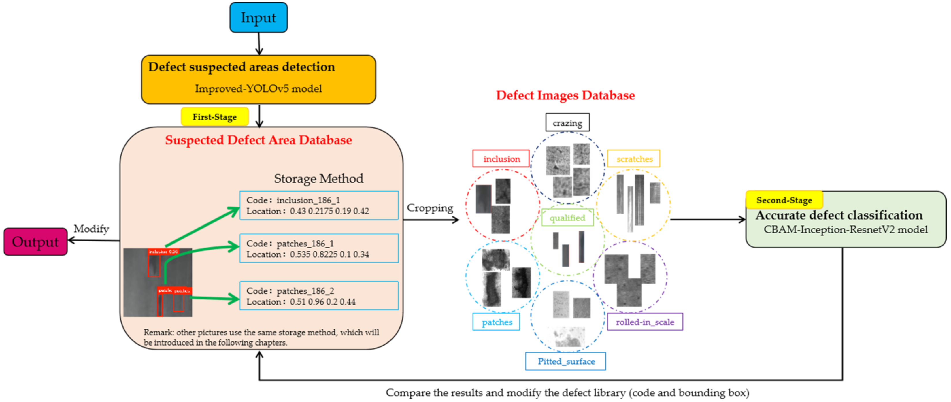
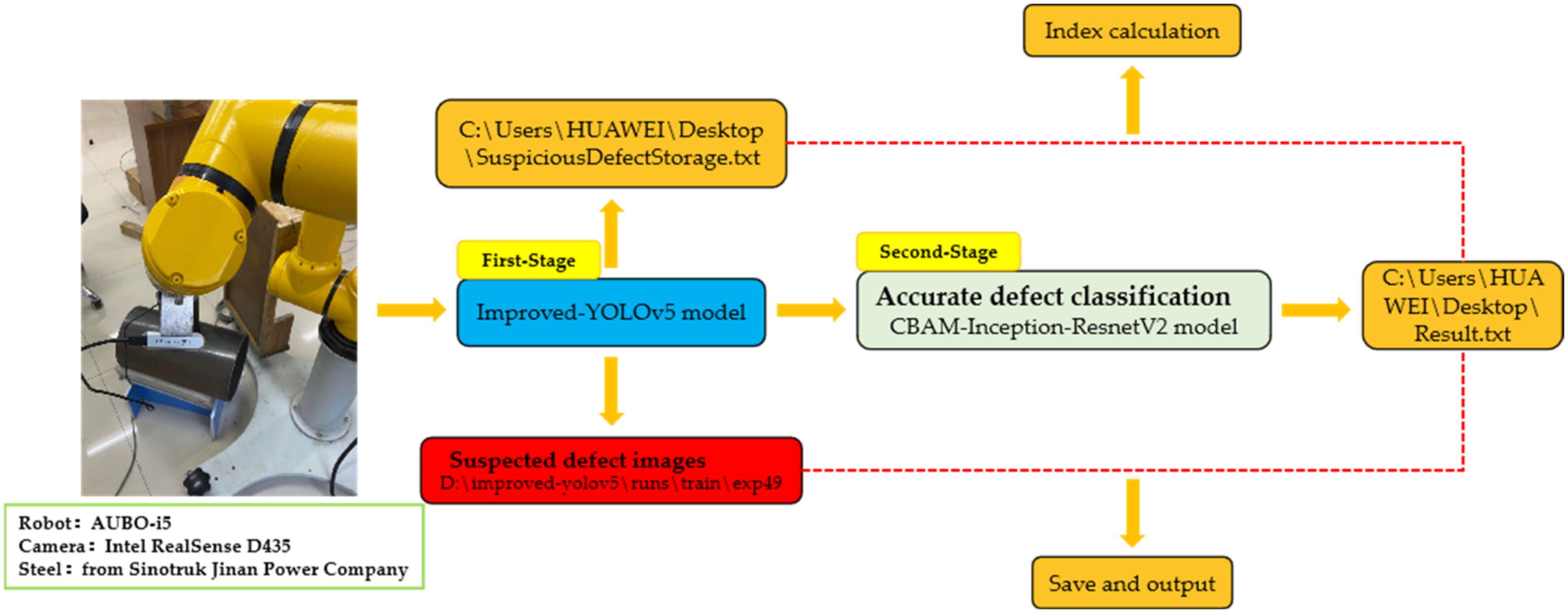
In response to the above problems, a two-stage defect detection framework based on Improved-YOLOv5 and Optimized-Inception-ResnetV2 is proposed. It completes detection and classification tasks through two specific models. The steps are shown in Figure 1.

Step 1: First-stage recognition: obtain suspected defect areas on the surface of the steel through the trained Improved-YOLOv5 module. The precise positioning of the defect area on the steel surface is completed.

Step 2: Crop the suspected defect areas and map them to the uniform size. Each image may have one or more suspected area data groups, which are stored in the defect images database.

Step 3: Second-stage recognition: use the Optimized-Inception-ResnetV2 module, obtained through transfer learning, to provide image recognition services, perform secondary recognition of these suspected area groups, and obtain the final result, which is used as the final judgment result of the suspected defect area.

Step 4: Compare the detection result in the suspected defect area database with the result after the secondary recognition. If the two are the same, directly output the results in the suspected defect area database; if the results are different, modify the results stored in the database and output them.

If a single model is used for the target detection, it is necessary to find regions of interest (ROIs) in an entire image, which can be complicated by useless background information. The precise location of the defect area through the first-stage recognition reduces the interference of more background information on the defect features, so the second-stage recognition results are more accurate and the performance of the model is better. Accurate recognition after defect target positioning not only realizes the two-stage recognition of insignificant defects, but also solves the problem of similar features between defects to a certain extent, which makes the results more credible. At the same time, in order to more effectively locate the insignificant minor defects with high similarity on the steel surface, this paper improves YOLOv5 detection methods from three aspects. Firstly, improve the feature extraction capability of the backbone network, and further optimize the feature scales of the feature fusion layer and multiscale detection layer. In order to better extract defect features and achieve accurate classification, we integrated the convolutional block attention module (CBAM) attention mechanism module with the Inception-ResnetV2 model, which can independently learn the weights of different channels to enhance attention to the key channel domain. We further optimized the loss function of the benchmark model, adding L1 and L2 regularization to reduce the variance and reduce the occurrence of overfitting.

3. Improved-YOLOv5: Suspected Defect Area Detection

3.1. The YOLOv5 Model

YOLO is a target detection algorithm based on regression. After inputting the images or video into the deep network, YOLO completes the prediction of the classification and location information of the objects according to the calculation of the loss function, so it makes the target detection problem transform into a regression problem solution [10].

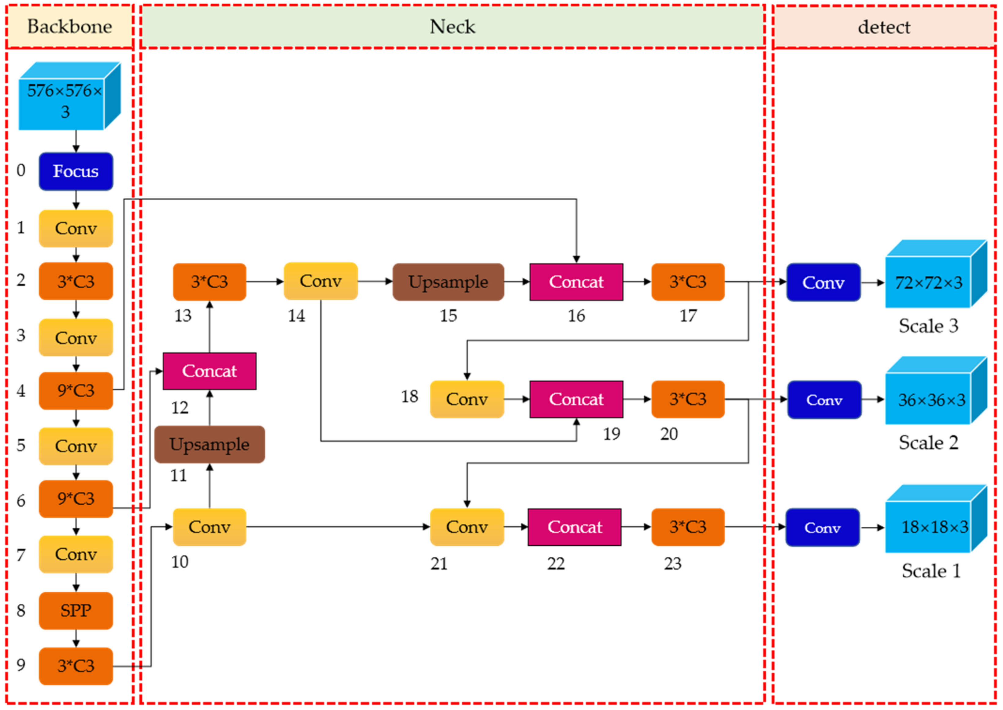
YOLOv5 [11] is based on the YOLO detection architecture and uses the excellent algorithm optimization strategy in the field of convolutional neural networks in recent years, such as auto learning bounding box anchors, mosaic data augmentation, the cross-stage partial network, and so on; they are responsible for different functions in different locations of the YOLOv5 architecture. In the architecture, YOLOv5 consists of four main parts: input, backbone, neck, and output. The input terminal mainly contains the preprocessing of the data, including mosaic data augmentation [12] and adaptive image filling. In order to adapt to different datasets, YOLOv5 integrates adaptive anchor frame calculation on the input, so that it can automatically set the initial anchor frame size when the dataset changes. The backbone network mainly uses a cross-stage partial network (CSP) [13] and spatial pyramid pooling (SPP) [14] to extract feature maps of different sizes from the input image by multiple convolution and pooling. BottleneckCSP is used to reduce the amount of calculation and increase the speed of inference, while the SPP structure realizes the feature extraction from different scales for the same feature map, and can generate three-scale feature maps, which helps improve the detection accuracy. In the neck network, the feature pyramid structures of FPN and PAN are used. The FPN [15] structure conveys strong semantic features from the top feature maps into the lower feature maps. At the same time, the PAN [16] structure conveys strong localization features from lower feature maps into higher feature maps. These two structures jointly strengthen the feature extracted from different network layers in Backbone fusion, which further improves the detection capability. As a final detection step, the head output is mainly used to predict targets of different sizes on feature maps. The YOLOv5 consists of four architectures, named YOLOv5s, YOLOv5m, YOLOv5l, and YOLOv5x. The main difference between them lies in the number of feature extraction modules and convolution kernels at specific locations on the network. The network structure of YOLOv5 is shown in Figure 2.

The defects on the steel surface are irregular in shape, random in location, and different in size; moreover, there are often a large number of targets with smaller scales. Under these circumstances, the original YOLOv5 model cannot fully meet the detection requirements, and there are situations such as low detection accuracy and missed detection. Therefore, this paper improves the original YOLOv5 network model. Firstly, we modified the backbone network, embedded an attention mechanism module to strengthen more important information, and reduced the interference of irrelevant information so as to improve the feature extraction ability of the model and improve the accuracy of defect detection. According to the distinguishing feature of small defect targets in steel, we further optimized the feature scales of the feature fusion layer and multiscale detection layer, so that the detection model could better adapt to the target detection of small defects, which improves the defect detection performance.

3.2. Improved Backbone

The backbone network of YOLOv5 is a convolutional neural network that extracts feature maps of different sizes from the input image by Focus slice, BottleneckCSP, and SPP modules [17]. The feature extraction capability of the backbone network directly affects the detection performance of the entire model.

For a deep convolutional neural network, the overall structure is an inverted pyramid, and the size of the feature map is scaled with the entire network structure—that is, the deeper the network, the smaller the feature map. Therefore, for small targets in the image, their feature information may be assimilated by the feature information around the area due to the pooling and downsampling operation, then disappear. As for defects on the surface of the steel, it is often insignificant relative to the entire surface. If large-scale downsampling is performed, it will cause the loss of its own semantic information, and may lead to missed detection.

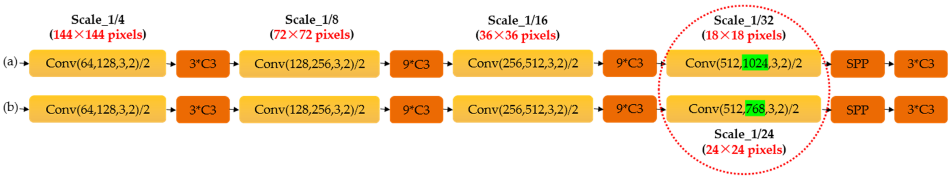
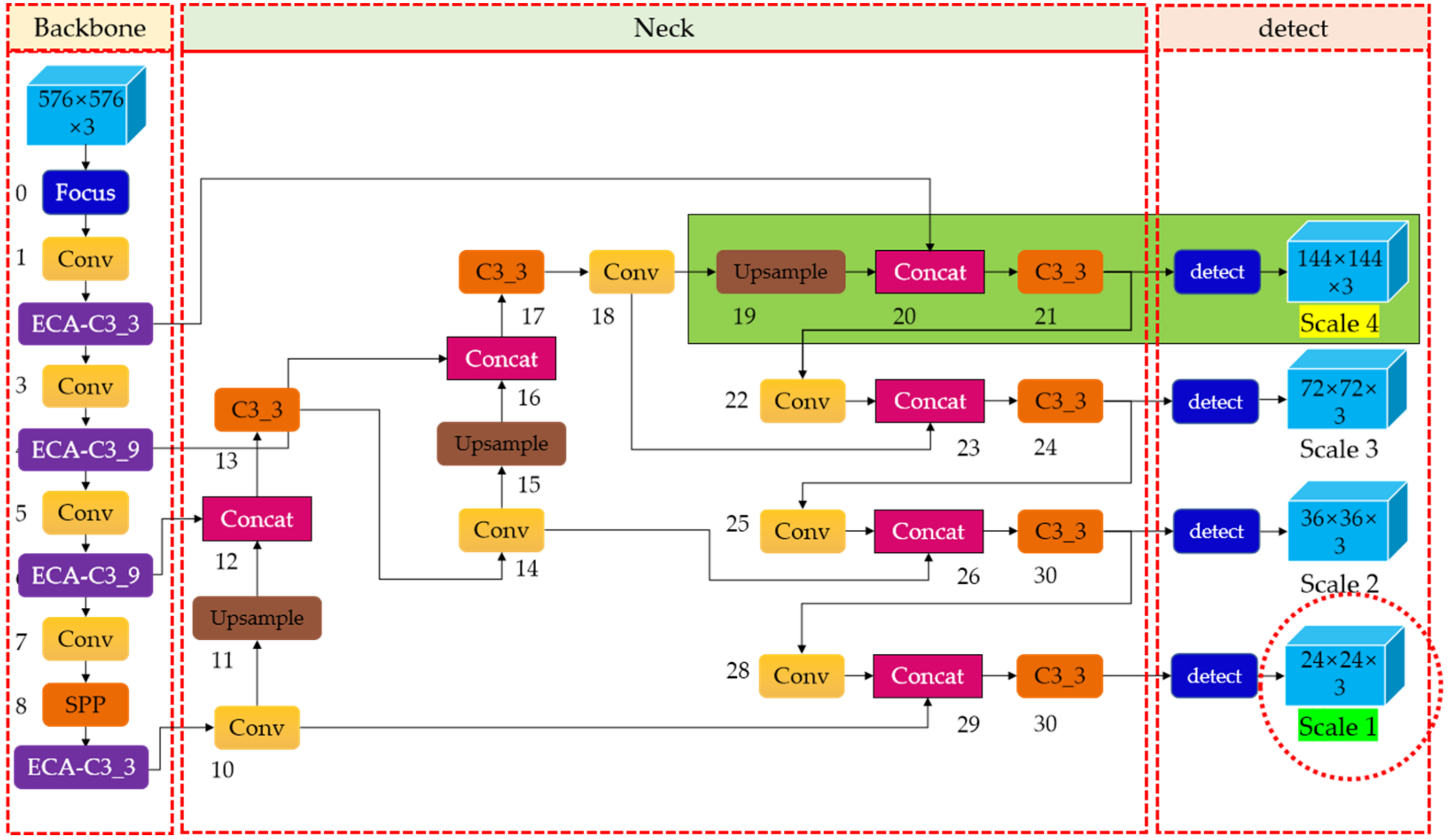
In order to avoid a substantial loss of defect semantic information and, improve the feature extraction capability of the backbone network for steel defects, we removed the Conv and C3 layer that obtained 1/32 scale feature information (refers to the size of feature maps generated is 18 × 18 pixels) in the original YOLOv5, and replaced it with a Conv and C3 layer that extracted feature information at a 1/24 scale (i.e., the size of feature maps generated is 24 × 24 pixels). With this modification, after the feature information generated by the shallow network was fused with the deep information, a 1/24-scale detection head (one level lower than the original YOLOv5, represented as Scale 1 with the green background, surrounded by a red circle) was formed to detect large-scale targets. We know that YOLOv5 generates feature maps of large, medium, and small scales, so in this way, the size of the large-scale feature map extracted by the model was reduced by one level, which reduced the interference of large-scale useless information, and improved the detection accuracy. The backbone network before and after modification are shown in Figure 3.

3.3. The Attention Mechanism

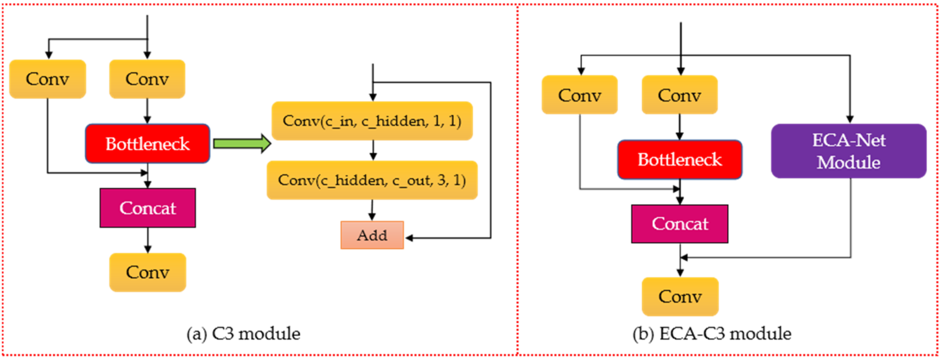
The morphological features contained in feature maps of different scales, which are extracted by the backbone network, included not only foreground objects, but also background information. For small targets, the foreground information in the feature map is sparser. In order to help YOLOv5 ignore confusing information and focus on useful target objects, we embedded an efficient channel attention network (ECA-Net) [18] mechanism into the backbone network, connected it in parallel to the C3 module, and named it ECA-C3. Next, we replaced the C3 module in the original YOLOv5 backbone network with the ECA-C3 module. Figure 4a,b show the architecture of the C3 module and ECA-C3 module, respectively.

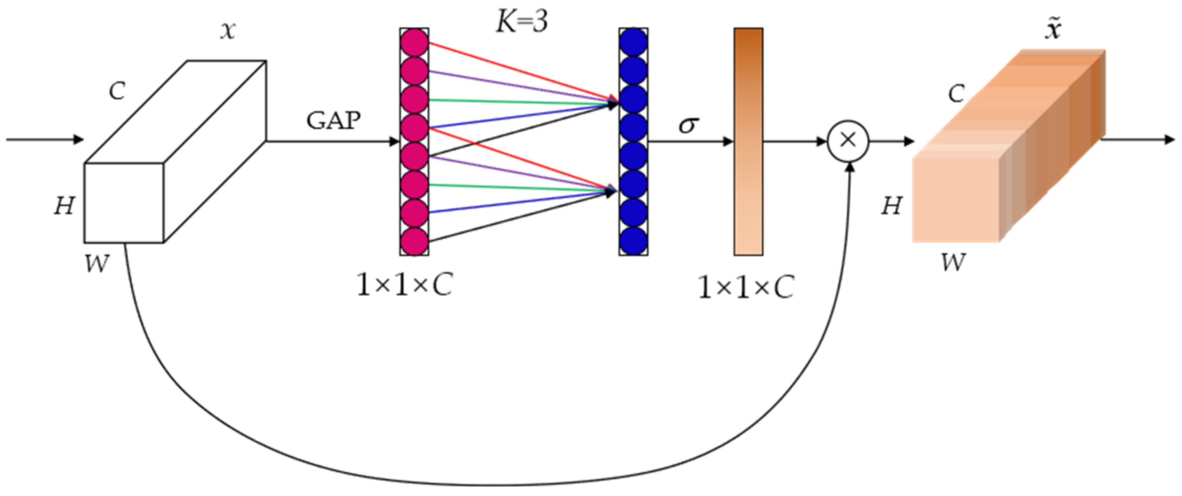
The efficient channel attention network (ECA-Net) is a local cross-channel interaction strategy without dimensionality reduction. At the same time, it can also adaptively select the size of the one-dimensional convolution kernel. The ECA module effectively captures information about cross-channel interactions and obtains a significant performance increase. Figure 5 shows the structure diagram of the ECA module.

In order to make the neural network learn the attention weights of each channel adaptively, ECA-Net captures local cross-channel interaction information by considering each channel and its K neighbors. The convolutional kernel size K represents the coverage of local cross-channel interactions, i.e., how many neighbors of that channel are involved in the attention calculation. K is related to the channel dimension C, as long as the channel dimension C is given, the kernel size K will be adaptively determined as shown in Equation (1):

$$\mathrm{K}=\mathsf{\Psi }\left(\mathrm{C}\right)={\left|\frac{{\log }_2\left(\mathrm{C}\right)}{\mathsf{\gamma }}+\frac{b}{\mathsf{\gamma }}\right|}_{odd}$$

(1)

where C is the channel dimension, ${\left|t\right|}_{odd}$ denotes the nearest odd number of $t$; $\mathsf{\gamma }$ is set to 2 and b to 1.

A one-dimensional convolution operation is performed on the obtained convolution kernel, and the sigmoid activation function is used to get the weights of each channel. The equation is as follows:

$${\omega }_C=\sigma (C1D_k(y)),$$

(2)

where ${C1D}_k$ represents a one-dimensional convolution operation with a kernel of K, $\sigma$ is the sigmoid activation function, whose calculation formula is $\sigma =\frac{1}{1+e^{-z}}$, y represents the different channels, ${\omega }_c$ is the weights of each channel generated, and its dimension is 1 × 1 × C.

Finally, the generated attention weights and input feature maps are weighted and summed, so that the extracted features are more directional, which makes these features able to be more fully utilized. The weighting equation is as follows:

$$X_c{=X}_c \otimes { \omega }_c,$$

(3)

where $\otimes$ represents multiplying element by element, and $X_c$ is the output result after passing the ECA module.

As we can see that the ECA attention module embedded in the backbone network is represented by the purple module in Figure 6.

3.4. Increasing Scale of Model Prediction

As for steel defect detection, the difficulty is that the defect area is too small relative to the entire steel surface, which makes defect features not obvious when the images are not enlarged. In order to solve this problem, we made the following improvements to the architecture of the feature fusion layer and detection layer.

As seen in the previous section, in the target detection process, shallow features are conducive to the detection of small-scale targets, while deep features are more conducive to large-scale target detection. In the feature fusion layer and detection layer network, the feature pyramid network (FPN) and the pixel aggregation network (PAN) [16] architectures are used to strengthen the feature fusion capability and transferability of positioning. Finally, there are three feature fusion layers that generate three scales of new feature maps with sizes of 72 × 72 × 255, 36 × 36 × 25, and 18 × 18 × 255; the three output detection layer scales corresponding to them are 1/8, 1/16, and 1/32, respectively, for the detection of small, medium, and large goals.

As shown in Figure 6, we added the 1/4-scale detection layer marked with the green background to generate 144 × 144 feature maps to capture shallower feature information on the steel surface. This scale detection head is represented as Scale 4 with the yellow background in Figure 6. The new fusion layer starts to strengthen the features from the second layer of the backbone network, which eliminates the shortcomings of the original YOLOv5 model that does not make full use of the shallow features. With this improvement, the features of the shallower network can be reused in the deeper network. Therefore, the newly added prediction head at the end of the network can generate low-level and high-resolution feature maps, which are more sensitive to small targets, thus improving small object detection.

4. Optimized-Inception-ResnetV2: Accurate Defect Identification

After Improved-YOLOv5 model defect detection, we obtained images with bounding box and classes, and saved them in the suspected defect area database. Next, we cropped the suspected defect area surrounded by the bounding box. Then we obtained one or several groups of suspected defect area groups from each image after cropping. Furthermore, we numbered these suspected defect area groups, so as to directly locate the position of the suspected defect area in the original image during subsequent modification. The numbering method was composed of three parts: the type of the defect, the serial number of the original image, and the serial number of defects, such as patches_186_2. We used the Optimized-Inception-ResnetV2 model obtained by transfer learning to classify these suspected defect area groups, and regarded it as the final judgment result of the suspected defect area. Then we found the bounding box and class of the image in the corresponding suspected defect area database according to the number of each suspected defect area group, modified it in terms of the two-stage recognition comparison result for further industrial processing, and output the final result.

4.1. The Inception-ResnetV2 Model

The Inception-Resnet [19] architecture, proposed by Szegedy, is a mixture of Inception and Resnet network backbone architectures. The Inception module is a network with good local topology, i.e., multiple convolution or pooling operations are performed on the input image in parallel. It does not restrict itself to a specific convolution kernel, but uses all convolution kernels of different sizes at the same time, and then merges all convolution output results to form a deeper feature map. Taking advantage of that can lead to better image representation [12]. Resnet [20] is a residual neural network architecture with a depth of 152 layers, proposed by Kaiming He in the ImageNet competition. He introduced a shortcut architecture in the neural network. Specifically, this means adding the input layer transfer and convolution results, which reduces the problems of a neural network such as the gradient dispersion caused by rather deep depth.

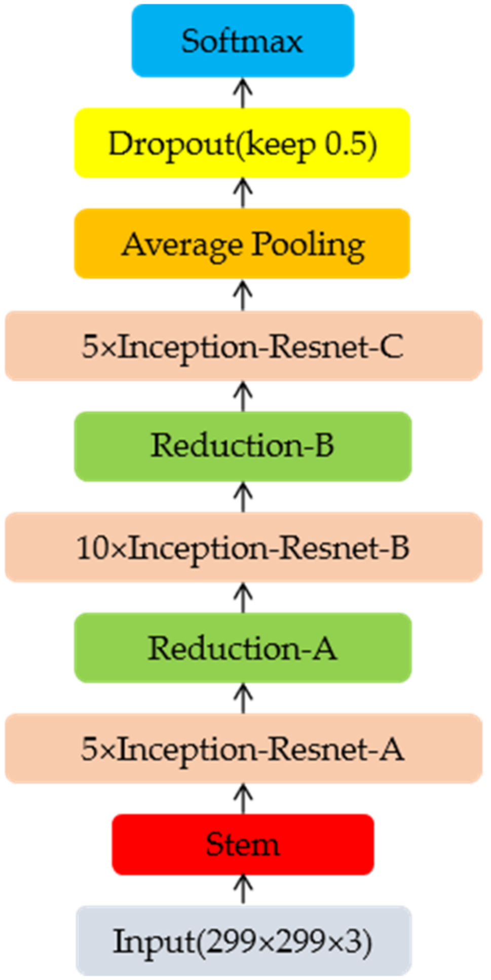
As shown in Figure 7, the Inception-ResnetV2 network redefines the input image size to 299 × 299 × 3, so as to maximize the recognition ability of graphics. The Stem architecture adopts the parallel structure and decomposition idea in the InceptionV3 [21] model, which can reduce the amount of calculation with little information loss. The 1 × 1 convolution kernel in the structure is used to reduce the dimensionality. Inception-Resnet-A, Inception-Resnet-B, and Inception-Resnet-C architectures adopt the Inception + residual network design, with deeper layers, more complex architecture, and more channels to obtain feature maps. The three architectures, Reduction-A, Reduction-B, and Reduction-C, are used to reduce the amount of calculation and the size of the feature map. The Inception-ResnetV2 model integrates the advantages of the Inception module and the residual network structure, which not only can increase the depth and width of the network but also avoid the disappearance of the gradients. 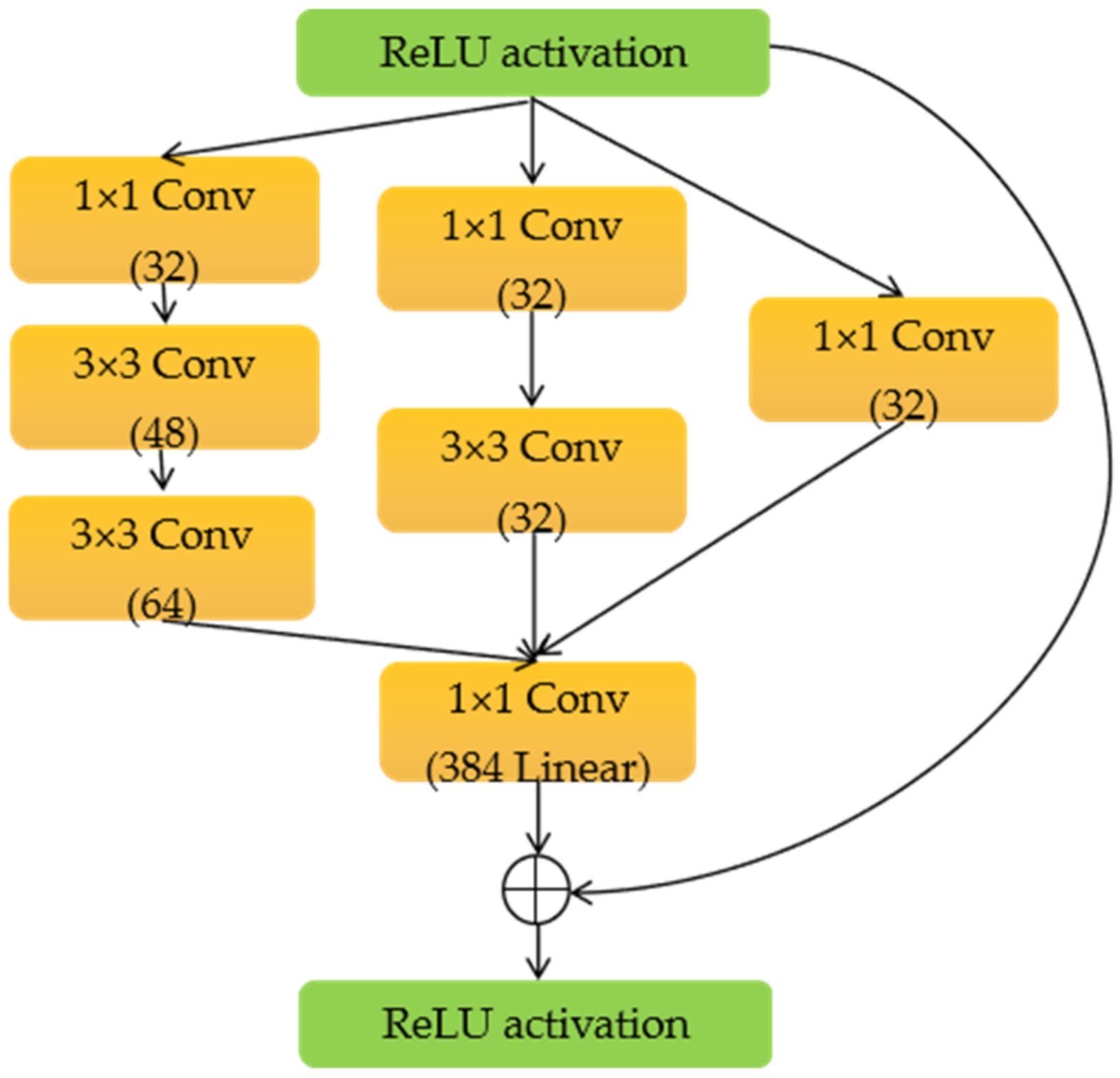Figure 8 shows the architecture of Inception-Resnet-A; the others are similar.

4.2. The CBAM Attention Mechanism

In order to save resources and obtain the most effective information quickly, the attention mechanism has become a very effective method to improve the feature extraction capabilities of neural networks. It can focus limited attention on key information and ignore other useless information automatically. 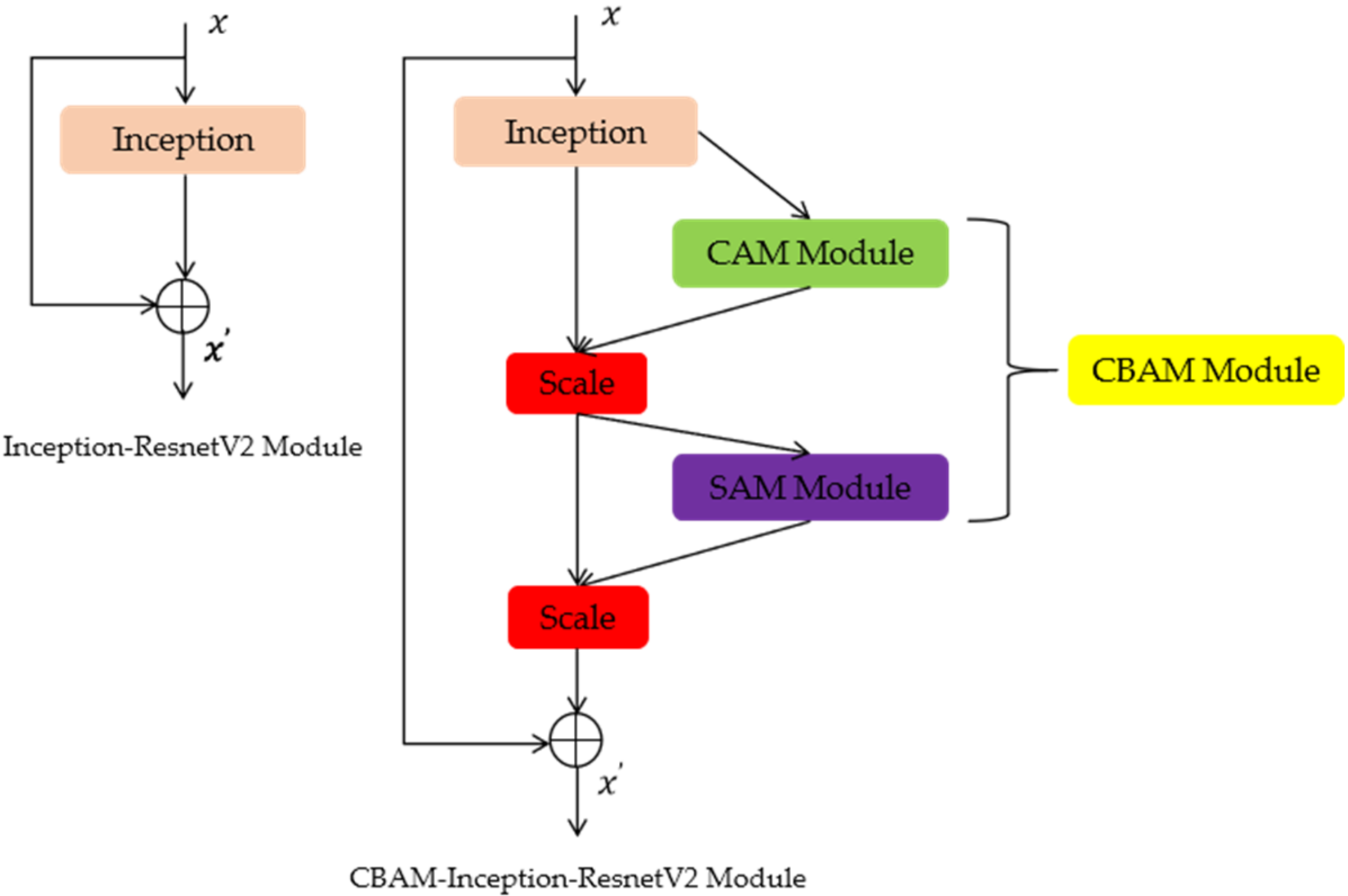In order to better extract defect features and achieve accurate classification, we embedded the convolutional block attention module (CBAM) mechanism [22] module in Inception-Resnet-A, Inception-Resnet-B, and Inception-Resnet-C of the Inception-ResnetV2 network. The specific architecture is shown in Figure 9.

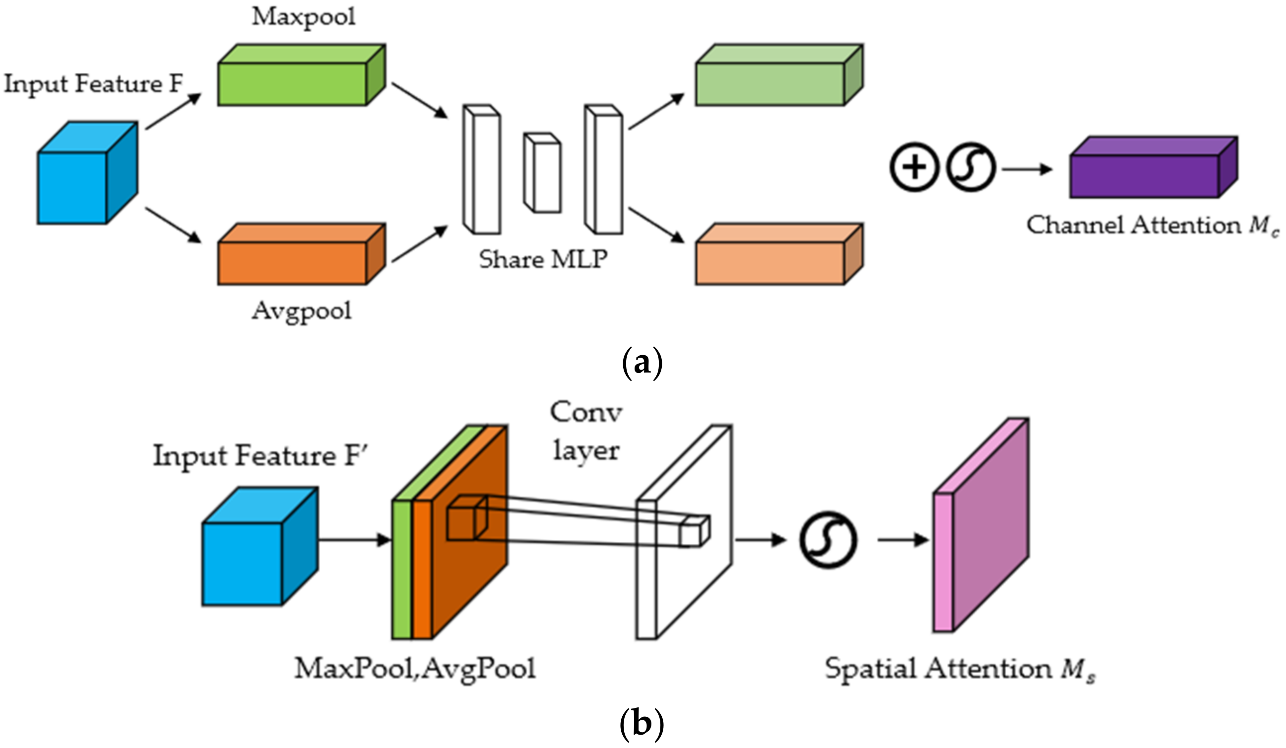
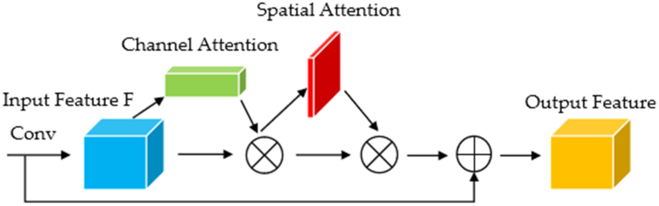
As shown in Figure 10, CBAM contains two independent submodules, a Channel Attention Module (CAM) and a Spatial Attention Module (SAM). They perform channel and spatial attention, respectively, emphasize important features, and suppress general features, which achieves the purpose of improving the target detection effect. This not only saves parameters and computing power [23], but also ensures that it can be integrated into the existing network architecture as a plug-and-play module.

Figure 11a shows the calculation process of CAM. For the input feature map, H, W, and C indicate the length, width, and number of channels, respectively. We can calculate the weight of each channel according to the following equation:

$$M_c\left(F\right)=\sigma (MLP\left(AvgPool\left(F\right)\right)+MLP\left(MaxPool\left(F\right)\right){=\sigma (W}_1\left(W_0\left(F_{avg}^c\right)\right){+W}_1\left(W_0\left(F_{max}^c\right)\right))$$

(4)

Each channel of the input feature map $F$ undergoes max pooling $F_{max}^c$ and average pooling $F_{avg}^c$ at the same time, and then passes through a Multilayer Perceptron (MLP). Next, element-wise addition is performed on the feature vector output by the MLP, and finally, the sigmoid activation function $\sigma$ is performed. Through this process, we can obtain the channel attention.

Figure 11b shows the calculation process of SAM. Taking the feature map output by the CAM module as the input, max pooling and average pooling are performed in sequence, and then a convolution operation is performed on the obtained intermediate vector. After taking the obtained convolution results to pass the sigmoid activation function $\sigma$, we can obtain the spatial attention, as shown in Equation (5):

$$M_s\left(F\right){=\sigma (f}^{7\times 7}\left(AvgPool\left(F\right)\right); \left(MaxPool\left(F\right)\right){)=\sigma (f}^{7\times 7}{(F}_{avg}^c{; F}_{max}^c\left)\right).$$

(5)

4.3. Optimization of Model Parameters

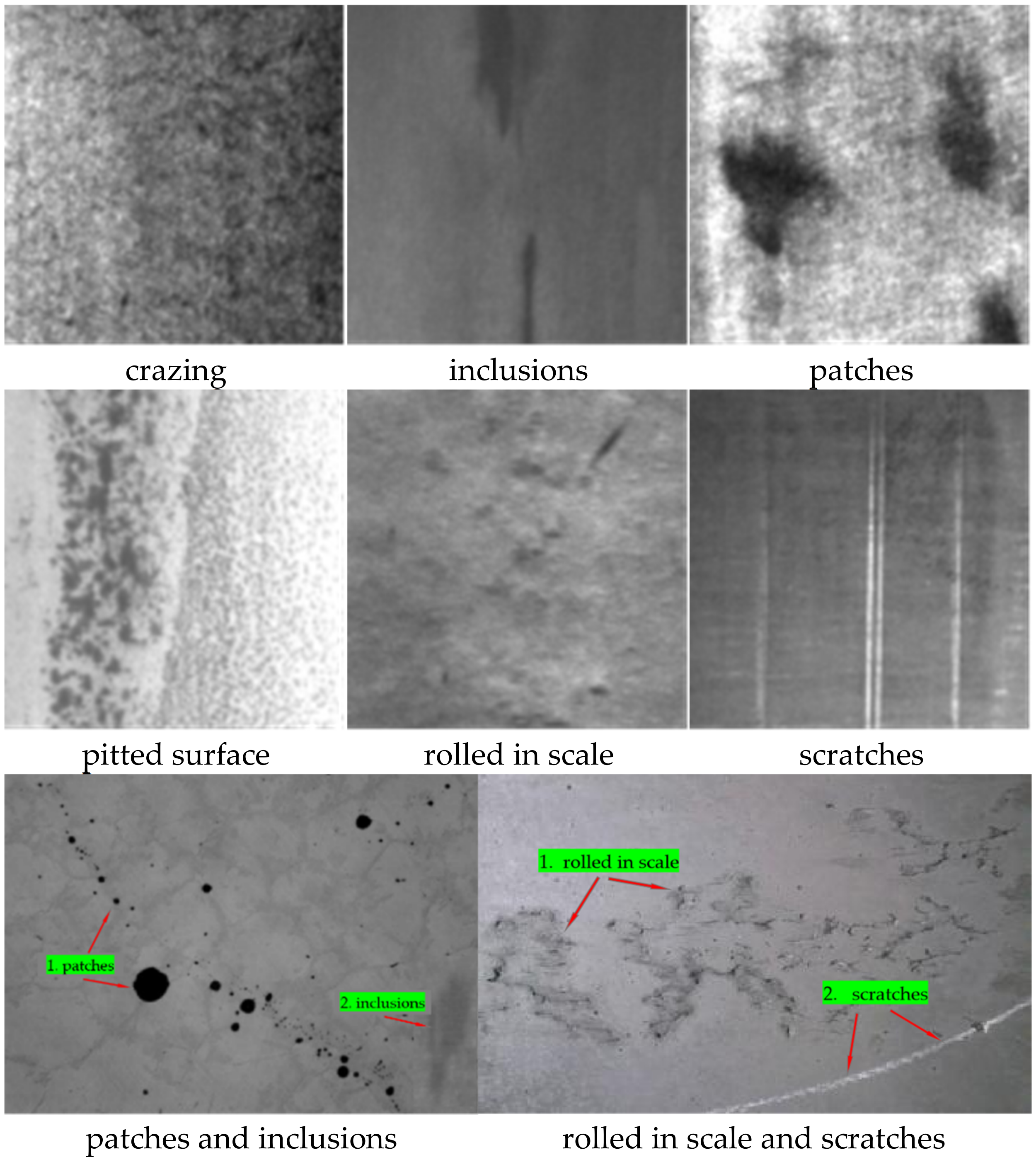
(1) In order to reduce the number of parameters of the model, we simplified the model, and reduced the number of Reduction-A, Reduction-B, and Reduction-C to three, five, and three. The last layer is the Softmax layer, but the output size depends on the specific problem. In this paper, there are six types of defects on the steel surface.

(2) We use the cross-entropy loss function [24] as the cost function. However, it can be seen from the foregoing that the similarity of industrial defects is relatively high and the defects are often not obvious, so it is easy to cause overfitting during training. Therefore, we added L1 and L2 mixed regularization to the loss function to avoid this phenomenon and make the model more robust when it is used in an industrial environment.

The optimized loss function $\mathrm{L}\_\mathrm{loss}$ is as follows:

$$\mathrm{cross}\_\mathrm{loss}=\mathrm{H}\left(\mathrm{p},\mathrm{q}\right)=-{\displaystyle \sum }_{\mathrm{x}}\mathrm{p}\left(\mathrm{x}\right)\mathrm{lnq}\left(\mathrm{x}\right)$$

(6)

$$\mathrm{L}\_\mathrm{loss}=\mathrm{cross}\_\mathrm{loss}+{{\displaystyle \sum }}_{\mathrm{i}}(\mathsf{\alpha }\left|{\mathsf{\omega }}_{\mathrm{i}}\right|+\left(1-\mathsf{\alpha }\right){\mathsf{\omega }}_{\mathrm{i}}^2),$$

(7)

where p represents the actual probability distribution of x, q represents the predicted probability distribution of x, ${\mathsf{\omega }}_{\mathrm{i} }$ represents weights, and $\mathsf{\alpha }$ represents the regularization parameter. The average of the cross entropy is calculated in the entire batch to get corss_loss, and then L1 and L2 mixed regularization is performed to reduce overfitting.

5. Results and Analysis

5.1. Datasets

In order to evaluate the two-stage defect detection framework proposed in this paper, we use three datasets: VOC2007 [25], Northeastern University’s public dataset NEU-DET, and its derived dataset Enriched-NEU-DET. There were 1800 pictures in total. Of these, there were 300 pictures of six kinds of defects. The six defects were marked as “crazing,” “inclusion,” “patches,” “pitted_surface,” “rolled-in_scale,” and “scratches.” The algorithm proposed in this paper firstly needs to train the Improved-YOLOv5 model and Optimized-Inception-ResnetV2 model to obtain the trained weight file for the first-stage and second-stage recognition. The datasets used in training are Enriched-NEU-DET and NEU-DET, divided into a training set, test set, and validation set in a ratio of 6:2:2.

Since there is only one type of defect in each picture in the NEU-DET dataset, if a part of it is randomly selected to train Improved-YOLOv5, and then we complete the first and second defect recognition, step 4 (result comparison and modification in Section 2) can be removed, which diminishes the superiority and engineering practicability of the model proposed in this paper. At the same time, we wanted to further expand the dataset. Therefore, we made a further improvement to the NEU-DET dataset. First, we randomly sampled 600 images in the training set, and then used data augmentation methods such as horizontal flip, vertical flip, Mosaic technology [12], and random cropping included in YOLOv5. Finally, we expanded the dataset to 2000 sheets. In order to eliminate the limitation of the single defect type of each picture in the NEU-DET dataset, we went to a factory for field data collection. A total of 56 pictures with no fewer than two kinds of defects were collected. Data augmentation increased the sample size to 224 sheets. In the end, Enriched-NEU-DET had a total of 2224 image. Some of the images in the two datasets are shown in Figure 12.

Since the recognition process of the first stage plays a critical role in the detection performance, we made considerable improvements to YOLOv5. In order to further verify the superiority of our improved model, in addition to the above two datasets used in the training defect recognition framework, the VOC2007 dataset was also used to test whether the improved YOLOv5 had better performance on the commonly used dataset. VOC2007 contained 9963 labeled images, with 24,640 objects labeled in 20 categories, such as people, horses, dogs, apples, etc. It was a benchmark for the evaluations of the image classification and recognition methods. In our experiments, the VOC2007 dataset was divided into training and test sets in a ratio of 9:1, in the same way as the Enriched-NEU-DET dataset.

5.2. First-Stage Recognition

In the first-stage recognition process, we needed to use the best trained Improved-YOLOv5 model on Enriched-NEU-DET dataset, so the recognition accuracy of the Improved-YOLOv5 model was related to the performance of the entire framework. To validate the performance of the proposed improved YOLOv5, we first used the public VOC2007 and Enriched-NEU-DET datasets to conduct comparison experiments with YOLOv5, YOLOv4 [26], YOLOv3 [27], SSD [15], then a further ablation test was done in Enriched-NEU-DET.

5.2.1. The Evaluation Indexes

We used precision, recall, mAP (mean average precision), AP (average precision), accuracy, and FPS (frames per second) as measurement indicators. These metrics are defined as follows:

$$precision=\frac{TP}{TP+FP}$$

(8)

$$recall=\frac{TP}{TP+FN}$$

(9)

$$accuracy=\frac{TP+TN}{TP+FN+FP+TN},$$

(10)

where TP, FP, FN, and TN represent the number of true positives, false positives, false negatives, and true negatives, respectively. When the category of defect prediction is correct, and the intersection over union (IoU) is greater than a threshold (0.6 in our experiments), we consider the detection to be correct. The AP is the area under the precision–recall (P–R) curve. The mAP is the mean value of the AP of all categories. FPS represents the number of images that the target detection method can process per second, which can evaluate the real-time performance of the detection method. These can fully reflect the overall performance of the method.

5.2.2. Implementation and Settings

The environmental and configuration parameters of all experiments in this section are shown in

Table 1. Hardware and software parameters of the experimental platform.

Name	Parameter
Experimental platform	Tencent Cloud Server
CPU	8-Core
GPU	Tesla V100-NVLINK-32G
Operating system	Linux system
CUDA	Version 10.1
Deep learning framework	PyTorch 1.6.0
Language	Python 3.7.5

,

Table 2. Configuration of training parameter value for Comparison Experiment.

Parameters	The Size of Input Images	Optimizer	Learning Rate	Epochs	Batch Size	Momentum
Settings	576 × 576	Adam	0.01	300	32	0.9

,

Table 3. Configuration of training parameter value for Ablation Experiments.

Parameters	The Size of Input Images	Optimizer	Learning Rate	Epochs	Batch Size	Momentum
Settings	576 × 576	Adam	0.01	200	64	0.9

and

Table 4. The comparison results with related methods.

Dataset	Method	Precision						Recall	mAP	FPS
VOC2007	SSD	77.5%						67.4%	70.5%	46
	YOLOv3	74.9%						64.0%	64.8%	37
	YOLOv4	78.1%						69.5%	78.6%	35
	YOLOv5	82.6%						72.1%	79.2%	36
	Ours	84.9%						74.2%	81.3%	31
		AP
		a	b	c	d	e	f
Enriched-NEU-DET	SSD	41.2%	68.5%	77.8%	68.9%	47.3%	61.6%	59.0%	62.9%	13
	YOLOv3	33.4%	67.6%	77.2%	57.2%	46.9%	54.7%	51.5%	56.2%	35
	YOLOv4	53.9%	71.8%	79.4%	74.2%	49.0%	68.6%	69.8%	66.2%	31
	YOLOv5	52.4%	70.6%	83.6%	78.8%	61.8%	78.7%	71.4%	71.0%	29
	Ours	54.6%	79.6%	86.1%	92.3%	66.1%	89.6%	76.3%	78.1%	24

.

The training parameters have a certain impact on the performance of the trained model. Table 2 and Table 3 show the best configurations obtained after several training experiments.

5.2.3. Results of Comparison Experiment

From the results in Table 4, in addition to FPS, the Improved-YOLOv5 model proposed in this paper has better evaluation indicators than other target detection algorithms, but the model can fully meet the real-time requirements of the industrial detection process. The precision of Improved-YOLOv5 on the VOC2007 dataset is 2.3% higher than that of original YOLOv5, and the mAP value is also 1.5% higher. On the Enriched-NEU-DET dataset, the recall value is 4.9% higher than that of YOLOv5, and the mAP value is 7.1% higher, which shows that the improvement made by the YOLOv5 model for small target detection has a very good effect. These results show that the improved YOLOv5 detection method achieves the best result in terms of several evaluation indicators, and fully meets the requirements for further application in industrial production situations.

In the Table 4, a is “crazing,” b is “inclusion,” c is “patches,” d is “pitted_surface,” e is “rolled-in_scale,” and f is “scratches.”

5.2.4. The Results of Ablation Experiments

An ablation experiment is similar to the control variate method, which is an intuitive way to study causality. As we saw in the previous section, the improved YOLOv5 model in this paper leads to a certain degree of performance improvement. In order to verify whether the three improvements are all effective at improving performance, and whether there is any interaction between them, we conducted ablation experiments on the Enriched-NEU-DET dataset.

We use four schemes to represent different improvements to YOLOv5. The improvement schemes are shown in

Table 5. The improved schemes.

Schemes	ECA Module	Scale 4 Layer	Generate 24 × 24 Feature Maps	Generate 18 × 18 Feature Maps
1	×	×	×	√
2	√	×	×	√
3	√	√	×	√
4	√	√	√	×

.

“ECA module” refers to the embedded attention mechanism ECA module on the C3 module of the backbone network, which is marked with a purple square in Figure 6; “Scale 4 layer” refers to the model that adds the new feature fusion layer to YOLOv5, which is marked with a green background in Figure 6; “Generate 24 × 24 feature maps” removes the Conv and C3 layer that obtained 1/32 scale feature information, replacing it with a Conv and C3 layer that extracts feature information at a 1/24 scale.

• Scheme 1 is the original YOLOv5 mode;
• Scheme 2 refers to the model that further applies ECA attention mechanism to the model;
• Scheme 3 refers to the model that further adds the new feature fusion layer Scale 4 layer;
• Scheme 4 is the Improved-YOLOv5 model proposed in this paper.

The final test results of the four schemes are shown in

Table 6. The comparison results of four schemes.

Schemes	AP (%)						Recall (%)						mAP (%)
	a	b	c	d	e	f	a	b	c	d	e	f
1	52.4	70.6	83.6	78.8	61.8	78.7	53.6	71.1	87.0	72.4	53.8	71.6	71.0
2	52.8	72.2	84.7	83.9	63.3	80.1	54.1	74.5	87.1	76.9	60.3	74.8	72.9
3	53.1	76.9	86.6	93.0	66.9	84.3	56.2	78.8	88.9	79.9	68.7	79.0	76.8
4	54.6	79.6	86.1	92.3	66.1	89.6	57.7	80.9	88.9	79.6	67.9	81.4	78.1

. We use six letters to refer to the six types of surface defects: a represents “crazing,” b represents “inclusion,” c represents “patches,” d represents “pitted_surface,” e represents “rolled-in_scale,” and f represents “scratches.”

From Scheme 1 in Table 6, the mAP value of the original YOLOv5 is 71.0%. The mAP of Scheme 2 is 72.9%, which shows that the embedding of the ECA module has a certain positive impact on the network. Next, we tested Scheme 3. It shows that the new feature fusion layer works and contributes to defect detection. In particular, the recognition accuracy of “pitted_surface” defects increased by 9.1%, which reflects that most of the “pitted_surface” defects in the dataset are small-scale defects, and also reminds us that the steel production process needs to pay special attention to the occurrence of this type of defects. Finally, we tested the model in this paper and found that the performance of the overall model had been further improved. For instance, the mAP value increased by 1.3%. However, it can also be seen that the AP value and recall of three types of defects marked in italics decreased, which indicates that the three major improvements may interact with each other for the recognition of “patches,” “pitted_surface,” and “rolled-in_scale.”

In order to make the experimental results in Table 6 more intuitive, we visualized some of the recognition effects, as shown in Figure 13.

It can be clearly seen from Figure 13 that:

• From Scheme 1 to Scheme 4, more and more defects were identified in the images; there was almost no “missed detection” phenomenon in the six images of Scheme 4.
• Scheme 1 can only detect relatively large and clear targets in the images, while the detection effect of Scheme 2 is greatly improved for Scheme 1. Scheme 2 can accurately identify relatively fuzzy and dark targets, such as “inclusion” defects.
• It can be seen from the six images in Scheme 2 that, although the optimization effect of Scheme 2 is significant, there are obvious overlapping phenomena, such as “patches.” When the two defects are relatively close, Scheme 2 easily confuses them. Scheme 3 effectively improves the overlap phenomenon because it can identify and accurately locate two close targets. What is more, Scheme 3 can also identify small targets existing in large targets.
• Scheme 4 further optimizes the third option. Although the optimization effect is not as great as with the previous two improvements, for insignificant and illegible defects, such as “inclusion,” the effect of Scheme 4 is clear; it further reduces the missed detection of defects.

5.3. Second-Stage Recognition

Steel images are processed by the trained Improved-YOLOv5 model to identify the suspected defect areas, which are added into a suspected defect database for second-stage recognition. The second-stage recognition needs to use the best-trained Optimized-Inception-ResnetV2 model on the NEU-DET dataset, so the classification performance of the model is related to the output of the entire framework result.

We adopted a method of training based on transfer learning [28]. First, all the parameters of the convolutional layers are locked, then the global average pooling is connected, and next, the dropout layer is connected to prevent overfitting, where the parameter is set to 0.5. Finally, we connect the softmax classifier. The pretraining model is trained on the Imagenet1000 dataset by Inception-Resnetv2 as the basic model, and we directly transfer the basic model to NEU-DET dataset for training. The initial learning rate is 0.0002. When the training reaches the 60th epoch, the fine-tuning method of unlocking the convolutional layers locked previously is used to continue training to the 100th epoch, and to adjust the learning rate to 0.00002. In order to prevent randomness in the training process, multiple trainings are carried out, and, finally, the best parameter model is selected for testing.

The configuration of training parameters is shown in

Table 7. Configuration of training parameter values for Comparison Experiment.

Parameters	Size	Optimizer	Lr	Epochs	Batch Size	Loss Function	Classifier
Settings	224 × 224	Nadam	0.0002	100	32	Cross entropy loss	Softmax

Remarks: Lr is learning rate, Size: size of input images.

.

Figure 14a,b show the changing situations for the recognition accuracy and the loss function with the epochs during the training process on the NEU-DET dataset. As can be seen from Figure 14a, at the 70th epoch, the recognition accuracy of the two models tends to be stable. The results show that the recognition accuracy of Optimized-Inception-ResnetV2 has improved compared with the original network model, by 3.57%. As can be seen from Figure 14b, when the training reaches the 61st epochs, the abovementioned fine-tuning method is adopted, then the loss function has a sudden fluctuation, then continues to decrease. This shows that fine-tuning during training can reduce the loss and improve the accuracy. We also know that the Optimized-Inception-ResnetV2 model reached the best state at the 75th epoch and began to stabilize (in the original model this was at about the 85th epoch). This shows that the training convergence speed of Optimized-Inception-ResnetV2 is significantly faster than the Inception-ResnetV2 model. This is because the CBAM module can effectively suppress the interference of useless features and redefine the importance of each channel and spatial feature. This makes the network stable faster and gives it a better performance.

In order to further investigate the ability of the Optimized-Inception-ResnetV2 model to identify various types of defects and the details of defect misjudgment, a multiclassification confusion matrix was introduced to quantitatively analyze the training and testing status of the NEU-DET dataset described above. A confusion matrix comprehensively reflects the recognition accuracy and the misjudgment of real defect types. The quantization diagram of the confusion matrix of Optimized-Inception-ResnetV2 model and Inception-ResnetV2 model is shown in Figure 15. It can be seen that the optimized model is significantly better than the original model, and the confusion between different types of defects is lower. We know that “crazing” and “scratches” are the two most easily confused types in the recognition process, and there may be misjudgments between the two. This is because the “scratches” are mostly concentrated in one direction in our dataset; however, the “crazing” is in all directions. The two classes are relatively similar, and so it is easy to mistakenly identify “crazing” in a specific direction as “scratches.” Therefore, in future research, we can try to perform data augmentation on “scratches” and “crazing,” increase the gap between the two classes, and further improve the recognition accuracy.

In order to demonstrate the superiority of the classification model proposed in this paper, we conducted a comparative experiment with the VGG19 [29], Resnet50 [30], InceptionV4 [31], and Inception-Resnet-V2 algorithms. The results of the comparative experiment are shown in

Table 8. The comparison results of four algorithms.

Algorithms	Parameters (M)	Accuracy (%)
VGG19	39.0	69.42
Resnet50	25.6	73.60
InceptionV4	41.3	78.03
Inception-ResnetV2	28.9	78.76
Optimized-Inception-ResnetV2	37.7	82.33

. They show that the network Optimized-Inception-ResnetV2 proposed in this paper can significantly improve the model recognition rate and improve the network performance at the cost of a small parameter amount.

5.4. Simulation of Industrial Actual Defect Detection Environment

After the abovementioned training process, we obtained the model with the best performance for the first-stage and second-stage recognition.

In order to illustrate the advancement of the two-stage framework, we first conducted three sets of verification experiments with the Enriched-NEU-DATA dataset. It can be seen from

Table 9. Comparison results of two kinds of single-stage identification methods and the two-stage framework of this paper.

Method	mAP	mAP Increasing
Improved-YOLOv5	78.1%	—
Optimized-Inception- ResnetV2	69.7%	−8.4%
Two-stage recognition framework	83.3%	+5.2%

that, due to the single-stage model Optimized-Inception-ResnetV2 being a classification network, it is not suitable for a situation where an image has multiple different types of defects that require identification—an inevitable drawback. In addition, we found that the mAP value of the two-stage recognition is 5.2% higher than that of the single-stage recognition model Improved-YOLOv5. To sum up, the defect detection method proposed in this paper represents a breakthrough compared with the current mainstream defect detection method based on vision, and can be applied to complex and multitarget detection scenarios like the Enriched-NEU-DATA dataset. Therefore, our model improves the detection efficiency and accuracy.

In order to further verify whether the two-stage defect recognition framework proposed in this paper is effective in an actual defect detection environment, we built a simulation environment for industrial defect detection. The implementation process is shown in Figure 16.

We borrowed a number of discarded steels with defects from a factory. On this basis, we manually created several defects on the steels. The final number of various types of defects is shown in

Table 10. Comparison of simulated industrial defect detection results.

Number	10			6			6			6			10			16
Type	Crazing			Inclusion			Patches			Pitted_Surface			Rolled-In_Scale			Scratches
Index	TP	FP	P	TP	FP	P	TP	FP	P	TP	FP	P	TP	FP	P	TP	FP	P	Acc
A	9	1	0.90	4	1	0.67	6	0	1.00	4	2	0.67	8	1	0.80	13	3	0.81	0.80
B	5	3	0.50	3	1	0.50	5	0	0.83	3	3	0.50	5	3	0.50	10	6	0.63	0.56
C	9	1	0.90	5	1	0.83	6	0	1.00	5	1	0.83	9	1	0.90	16	0	1	0.91

.

• We used the AUBO-i5 robot to fix the Intel RealSense D435 industrial camera so that it could scan the steel surface by itself to complete the image collection of the steel surface, and take photos with robot teaching. At the same time, we used the exposure lamp to illuminate the steel.
• The images were sent to the first-stage recognition model in real time, allowing us to obtain images of the suspected areas of the defect; the details were written into a suspected defect area database (“C:\Users\HUAWEI\Desktop\SuspiciousDefectStorage.txt”).
• After each image was detected, one or more groups of suspected defects wase obtained, cropped, and filled to a uniform size.
• We performed second-stage recognition on the suspected areas, judged the final category of the defect, and wrote the obtained result into the “C:\Users\HUAWEI\Desktop\Result.txt”.
• We wrote a Python script to compare the results of the two levels and calculate the value of each indicator. We compared the types of defects in the two documents (“SuspiciousDefectStorage.txt” and “Result.txt”): if they are the same, TP + 1; otherwise, TN + 1. When all the defects were traversed, the final index was calculated. TP indicates the number of defects that are correctly identified; TN indicates the number of defects that are incorrectly identified. The precision value is TP/(TP + TN).
• If the results of the two-stage detection were the same, we directly output the image in the suspected defect area database; otherwise, the image was output after being marked for later processing of the surface defects of the steel.

In Table 10, A is the single-stage model Improved-YOLOv5, B is the single-stage model Optimized-Inception-ResnetV2, C is the two-stage defect recognition framework proposed in this paper, P is precision, and Acc is the mean of all P.

It can be seen from Equation (6) that the precision rate can be used to indicate how many defects of each type are successfully and correctly identified. Therefore, we used the precision rate to evaluate the performance of the three models. In an actual industrial environment, the recognition results of the three methods are as shown in Table 10. It is not hard to see that the recognition effect of a two-stage defect recognition framework is obviously better than that of the other two single-stage models. We regarded “number-TP-FP” as the number of missed defects, and found that there was almost no missed detection when using the method proposed in this paper. Therefore, our model can be successfully applied to steel production works.

6. Conclusions

The surface defects of steel were taken as the research object in this paper. A two-stage recognition defect detection framework was proposed in order to solve the problem of complex morphology, small size, and similar features.

• The Improved-YOLOv5 model was used to identify the defects on the steel surface. We obtained the suspected defect areas, and the Optimized-Inception-ResnetV2 model was used to perform second-stage recognition of these areas. According to the comparison results of first- and second-stage recognition, the inspection of the entire steel surface was completed.
• In order to further improve the recognition accuracy of each stage of the model, we made various improvements to the YOLOv5 and Inception-ResnetV2. Through many experiments and tests, we proved that the performance of our model improved significantly.
• The recognition effect of the two-stage recognition framework in the Enriched-NEU-DET dataset was higher than that of the single-stage model Improved-YOLOv5 by 5.2% (mAP), and the single-stage model Optimized-Inception-ResnetV2 by 13.6% (mAP).
• In order to verify the detection performance in an actual industrial environment, robots and industrial cameras were used to build real scenes. Based on a comparison, the defect detection performance advantages of the two-stage recognition framework were obvious, which shows the superiority and universality of the model proposed in this paper.
• From the above research, we see that some types have large differences within categories, and some defects have small gaps between categories. It is easy to cause misjudgments between them during the identification process. Therefore, in future research, corresponding data augmentation and other methods can be carried out on different types of defects to further improve the recognition accuracy.