Abstract
Proton range monitoring and verification is important to enhance the effectiveness of treatment by ensuring that the correct dose is delivered to the correct location. Upon proton irradiation, different positron emitting radioisotopes are produced by the inelastic nuclear interactions of protons with the target elements. Recently, it was reported that the 16O(p,2p2n)13N reaction has a relatively low threshold energy, and it could be potentially used for proton range verification. In the present work, we have proposed an analysis scheme (i.e., algorithm) for the extraction and three-dimensional visualization of positron emitting radioisotopes. The proposed step-by-step analysis scheme was tested using our own experimentally obtained dynamic data from a positron emission mammography (PEM) system (our developed PEMGRAPH system). The experimental irradiation was performed using an azimuthally varying field (AVF) cyclotron with a 80 MeV monoenergetic pencil-like beam. The 3D visualization showed promising results for proton-induced radioisotope distribution. The proposed scheme and developed tools would be useful for the extraction and 3D visualization of positron emitting radioisotopes and in turn for proton range monitoring and verification.
1. Introduction
It is well-known that protons have low lateral scattering and therefore deposit energy more locally when compared to photons [1,2,3,4,5]. Hence, the concept of proton range monitoring and verification is important to enhance the effectiveness of proton therapy treatment [6]. The dose deposition of protons increases with depth, and near the end of their range, it reaches its maximum, commonly referred to as the Bragg peak. Considering this, protons have a lower exit dose when compared to photons, which are used in conventional radiation therapy [7,8,9]. Therefore, protons are highly sensitive to spatial uncertainties [10], which makes range monitoring and verification crucial in therapeutic applications.
Considering proton range monitoring, several strategies have been proposed and investigated, with their own specific advantages and disadvantages [11]. Proton radiography and tomography have both shown promising results for proton range verification, but scattering reduces the resolution of the acquired images [12]. Other direct and cost-effective techniques that were reported in previous investigations are the ionoacoustics technique [13] and secondary electron bremsstrahlung (SEB) [14]. In addition, several investigators have recently studied Prompt Gamma Imaging (PGI) [15,16] for proton range verification and reported promising results. Another important technique for proton range monitoring and verification is auto-activation Positron Emission Tomography (PET) imaging, which is a non-invasive technique. The proton range is estimated by measuring annihilation photons generated by positron emitting radioisotopes such as 15O, 11C and 13N. These positron emitting radioisotopes are generated as a result of nuclear reactions induced by incident protons.
In 1969, Maccabee et al. [17] first proposed the use of the auto-activation PET technique for hadron range monitoring and verification. Later, the proposed auto-activation PET technique was experimentally investigated at a heavy ion therapy facility at the Lawrence Berkeley national laboratory [18]. Furthermore, this technique was found to be promising for monitoring the delivered proton dose in therapeutic applications [19]. There are various PET system configurations that have been used to measure annihilation photons generated by positron emitting radioisotopes in the auto-activation PET technique with the ultimate goal of proton range monitoring and verification [20,21,22,23,24]. For example, full-ring scanners [21,22], which were found to have high detection efficiency but at the same time to incorporate a full ring– ring PET system into beam delivery, which is technically tedious particularly when there are geometric constraints. Non-ring PET systems were developed to circumvent the drawback of full-ring scanners by providing a higher degree of freedom for better patient positioning and installation [25,26,27,28,29]. These non-ring PET systems include the DoPET (Dosimetry-PET) system [26], which is a compact prototype in-beam PET scanner [27], a compact planar PET prototype [28] and a modularized acquisition-based dual-head PET with wider detectors [29]. The main drawbacks associated with these non-ring PET systems are mainly the limited angular coverage and artifacts in the reconstructed images.
Another notable system that has higher spatial resolution and sensitivity compared to previously introduced systems would be the positron emission mammography (PEM) system, which is a dedicated PET system for detecting breast cancer [30]. The PEM system was first proposed by Thompson et al. [31] and inspired the development of several PEM systems such as Clear-PEM [32], composed of a dual-plate detector head composed of LSO (Lutetium oxyorthosilicate) crystals and designed to allow the breast and axilla region field of view (FOV); dual-head planar PEM [33], which has a parallel dual-planar detector geometry composed of LSO crystals and designed for greater flexibility in positioning the object into the FOV; the LBNL-PEM (Lawrence Berkeley National Laboratory-PEM) [34], which has a rectangular geometry, with four detector plates composed of LSO crystals surrounding the breast, and has depth of interaction (DOI) measurements capabilities; the Naviscan PEM flex system [35], which is a specially designed system with two opposite detector heads to fit on a stereotactic mammography unit, with the aim of allowing emission and transmission scans at the same time; the Elmammo (Shimadzu) dbPET (dedicated breast PET) system [36], developed by Shimadzu Co. and designed with three contiguous rings allowing a larger FOV and confirmed high resolution images with four layers of DOI measurement capability; and the Jefferson laboratory PEM system [37], designed to be mounted on a stereotactic biopsy table to perform PEM-guided biopsies.
We have developed a highly sensitive PEMGRAPH (Mirai Imaging Inc., Fukushima, Japan) that consists of a dedicated dual-head PEM system with Pr:LuAG (Praseodymium-dopped Lutetium Aluminum Garnet) crystal and was designed for breast cancer diagnosis [38]. The Pr:LuAG scintillator, with its high light yield, short decay time and good energy resolution, is preferred for angular coverage, while BaSO4 (Barium sulfate) is utilized as a reflector with the crystal to efficiently reflect scintillation photons from Pr:LuAG. PEMGRAPH showed a high spatial resolution of 2.0 mm (FWHM) in the plane parallel to the detectors [39] and a higher detection sensitivity for breast cancer compared with whole-body PET [40]. Our developed system was found to have higher spatial resolution and higher sensitivity when compared to other commercial PEM devices.
Recently, Cho et al. [41] reported that the 16O(p,2p2n)13N reaction has a relatively low threshold energy and it could be potentially used for proton range verification. As a result, the 13N creation may be extracted by computing the gradient between early and late PET scans, and it is found to be highly connected with the Bragg peak. In our recent work, we have employed the Monte Carlo technique to study the generation of the 13N radioisotope and its potential use to estimate the Bragg peak location in a simulated water-gel phantom [42]. In the present work, we have introduced an analysis scheme based on our recent experimentally obtained results from a cyclotron and the PEMGRAPH system for the three-dimensional (3D) visualization of positron emitting radioisotopes (particularly 13N). The present analysis scheme uses data obtained from the PEMGRAPH system from a proton irradiated phantom to provide the 3D distribution of positron emitting radioisotopes by using the spectral analysis (SA) approach. All necessary computer programs and raw data used in the present analysis scheme were made open source under the GPLv3 license, which allows users to freely modify, compile and distribute data without any restrictions. To the best of our knowledge, this is the first time such an extensive algorithmic scheme is being proposed, and this will be useful to enhance the effectiveness of proton range monitoring and verification.
2. Materials and Methods
2.1. Experimental Setup and Measurements
A homogeneous water-gel phantom was prepared by mixing agar powder (C14H24O9) and water, with a ratio of 1/100 (in gm) (agar powder/water). The container used was high-density polyethylene (HDPE) with dimensions of 8 × 10 × 16 cm3 and a wall thickness of 0.15 cm. The phantom geometry and PEMGRAPH are schematically shown in Figure 1. In addition, the material composition of the water-gel and HPDE container are listed in Table 1.
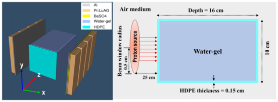
Figure 1.
Schematic diagram showing PEM heads and HPDE box containing water-gel being irradiated by a proton beam.

Table 1.
Density and material composition (fraction by weight) of HDPE container and water-gel used in the proton irradiation experiment and PEM scan.
The phantom was irradiated by a monoenergetic proton beam with 80 MeV energy for 60 s. The proton beam was pencil-like with a beam current of 10.20 nA and a diameter of ~1 cm produced by an azimuthally varying field (AVF) cyclotron at the Cyclotron and Radioisotopes Centre (CYRIC) facility at Tohoku University, Japan. Considering the current that was used, about 3.8 × 10¹² protons were used to irradiate the phantom. This value was higher than the typically used clinical beam, which was reported to be around 107 to 1010 protons. We have employed higher number of protons than those used in clinical irradiations mainly to obtain more counts during the PEM scan. It is also well known that proton-induced activity only depends on the target fragmentation. The experimental setup for the irradiation of the water-gel phantom is shown in Figure 2.
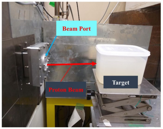
Figure 2.
Experimental setup of proton irradiation of water-gel phantom using a pencil-like proton beam with an energy of 80 MeV.
The distance between the proton beam port and water-gel phantom was set to 25 cm (see Figure 2). The proton beam was adjusted to irradiate the center of the water-gel phantom. Upon proton irradiation, different positron emitting radioisotopes are produced by the inelastic nuclear interactions of protons with the target elements. The water-gel was mainly composed of oxygen and carbon (note: hydrogen (1H) was not considered, mainly because it does not produce stable positron emitting radioisotopes). The list of major nuclear reactions and the positron emitting radioisotopes produced as a result of proton irradiation is shown in Table 2.
Table 2.
List of created isotopes, half-life, reaction and threshold reaction energy.
After proton irradiation, the irradiated water-gel phantom was placed in the PEMGRAPH system; this setup is shown in Figure 3. The irradiated water-gel phantom was scanned for 40 min with the PEMGRAPH system. The scanning of the irradiated water-gel phantom was started 15 min after the irradiation, mainly due to the time taken to carry the phantom from the irradiation room to the PEMGRAPH room after stopping the proton beam irradiation.
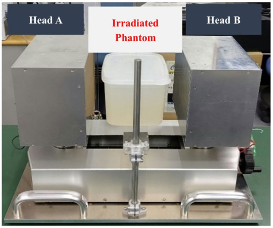
Figure 3.
Experimental setup of scanning the irradiated water-gel phantom using a dual-head PEMGRAPH system.
A prototype PEMGRAPH (Mirai Imaging Inc., Fukushima, Japan) system was employed to scan the irradiated water-gel phantom. The PEMGRAPH system is a highly sensitive and high-resolution open dual-head system [38] that consists of two planar 17.5 × 21.3 cm2 detector heads, each composed of four modules. There are a total of eight modules implemented in this device. The gap between each module was 0.6 cm. Each module was composed of 20 × 64 crystal array of Pr:LuAG with dimensions of 0.21 × 0.21 × 1.5 cm3 and was optically isolated by a BaSO4 reflector with a thickness of 0.1 cm. This adds up to a total of 20 × 64 × 8 = 10,240 Pr:LuAG crystal segments. Each side of the crystal matrix was optically coupled to three units of a 5.2 × 5.2 cm2 Hamamatsu H8500 position-sensitive photomultiplier tube (Hamamatsu Photonics Co., Ltd., Hamamatsu, Japan). The spatial resolution was 0.2 cm (at full width at half maximum (FWHM)) in the plane parallel to the detectors [38].
The acquired list mode data were reconstructed to 77 dynamic frames using the 3D iterative maximum likelihood-expectation maximization (MLEM) method [43,44]. The field of view (FOV) of each reconstructed image was 20.35 × 14.19 × 14.6 cm3, and the matrix size was 185 × 129 × 73. Therefore, the voxel size of each reconstructed image was 0.11 × 0.11 × 0.2 cm3. The experimental data were then analyzed using our previously developed PyBLD software [45] (link: http://www.rim.cyric.tohoku.ac.jp/software/pybld/pybld.html (accessed on: 11 January 2022)). AMIDE (A Medical Image Data Examiner) version 1.0.4 software was used to analyze the images (link: http://amide.sourceforge.net (accessed on: 11 January 2022)) [46]. The one-dimensional (1D), two-dimensional (2D) and three-dimensional (3D) time-course activities for 15, 20, 30 and 55 min after irradiation were obtained, which provided information on the location and distribution of activity.
2.2. The Spectral Analysis (SA) Approach
The spectral analysis approach employs an input function and exponential response function to identify kinetic components of a tracer [47,48]. The SA approach was initially developed for PET kinetics analysis, where it indicates a time-invariant single input/single output model used for the data quantification. During proton therapy, different radioisotopes of positron emitters such as 11C, 15O and 13N are produced by inelastic nuclear interactions of protons with the target elements. Considering that the radioactivity of each radionuclide is one component at time t and the time-activity A(t) of each voxel of the PEMGRAPH image, the concentration Cv(t), can be represented as
where is the convolution operation and A(t) is the time-activity input function of the system, presumed to be the impulse function in this study. The limit M represents the maximum number of terms to be included in the model and this is, in general, set to a large number, usually 1000. The values of βj are predetermined and fixed in order to cover an appropriate spectral range. For the studies involving short-lived positron emitting isotopes, this range needs to extend to the slowest possible event up to a value appropriate to transient phenomena. Each A(t) exp (−βj t) (impulse response function (IRF)) is pre-calculated. Subsequently, sets of αj values were solved using a non-negative least squares (NNLS) estimator. Once the IRFs are pre-calculated, the estimation sets of αj are entirely linear, and SA can instantly determine groups of αj without iterated computation.
Therefore, SA can be used for large datasets. To extract the short half-life (large β = 0.693/T1/2) 15O radioisotope, a range of β was used from 0.005 (athresh in spectral_analysis.py script) to 0.006 (betacut in spectral_analysis.py script) s−1, and for the 13N radioisotope, a range from 0.001 to 0.002 s−1 was used, respectively. On the other hand, for the longer half-life (small β = 0.693/T1/2) radioisotopes such as 11C, the range of β from 0.0005 to 0.0006 s−1 was used. We therefore computed the numerical Sv values for each voxel v with the threshold of αβ > 1.5 to remove the background region:
As a result, the SA approach can quickly calculate sets of α and β in each voxel. Few positive sets of β would be obtained that match the decay constants of the produced radioisotopes.
The SA technique was used to extract 11C, 15O and 13N positron emitting radioisotopes These were extracted separately from the merged images of 77 frames in different regions (see Figure 4). Firstly, the SA technique was applied to 3D merged images that contained 77 frames of 40 min images (from 15 to 55 min). Secondly, the time activity was calculated from the 3D data from 40 frames with 1 min intervals over 40 min using four separate regions of interest (ROIs): (1) whole, (2) edge, (3) plateau and (4) Braggpeak region, as shown in Figure 4. Then, the time activity data from 15 to 55 min (i.e., total 40 frames) were made into a single voxel image for each ROI. Figure 4 shows these four regions, together with their corresponding heights, widths and depths, respectively. The presence of proton-induced radioisotopes for each voxel was then confirmed using the obtained results.
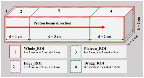
Figure 4.
The four regions of interests (ROIs) with their respective height (h), width (w) and depth (d) values used in the spectral analysis approach.
2.3. Scheme for Extraction and 3D Visualization of Positron Emitting Radioisotopes
The step-by-step algorithm of the proposed scheme for generating a 3D visualization of positron emitting radioisotopes is shown in Table 3. The algorithm summarizes the main steps for extracting and generating a 3D scatter plot of positron emitting radioisotopes. All the scripts, numerical tools and raw data used in the present scheme can be downloaded as Supplementary material from https://figshare.com/articles/software/An_analysis_scheme_for_3D_visualization_of_positron_emitting_radioisotopes_using_positron_emission_mammography_system/17171093 (accessed on: 11 January 2022).
Table 3.
The step-by-step algorithm of the analysis scheme for the extraction and 3D visualization of positron emitting radioisotopes using positron emission mammography.
3. Results
3.1. PEMGRAPH Measurements
In order to test the present scheme, we used 77 image frames reconstructed from the obtained 40 min of dynamic data using the PEMGRAPH system. Using the step-by-step scheme presented in Table 3, the 3D, 2D and 1D visualizations are shown in Figure 5. These were reconstructed along the beam direction for 15, 20, 30 and 55 min. In Figure 5, the normalized intensity is displayed along the y-axis. These were normalized with respect to 15 min after irradiation. From the images and 1D profiles shown in Figure 5, we observed two peaks along the beam direction: one at the proton beam entrance and the other near the distal dose Bragg region. In addition, a tail after the peak of the Bragg region was observed. These peaks decayed with time and remained visible for up to 55 min after the irradiation. Interestingly, the tail almost vanished after 30 min.
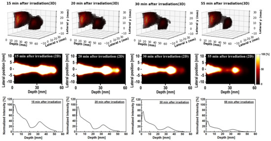
Figure 5.
The 3D (first row), 2D (second row) and 1D (third row) time−course activity covering 15 to 55 min data sets obtained from the PEMGRAPH measurements.
3.2. Spectral Analysis of PEMGRAPH Measurements
The spectral analysis (SA) approach was applied to the dynamic time-dependent activity data to quantify different positron emitting radioisotopes. The step-by-step procedure used for this analysis can be found in the proposed scheme shown in Table 3. The 2D images with their associated 1D profiles generated using the SA technique are shown in Figure 6. In Figure 6, the y-axis represents the normalized intensity for each radioisotope. The sum of all radioisotopes (shown as SA_sum in Figure 6), the 11C (shown as SA_11C in Figure 6) has two peaks—namely, (1) at the entrance and (2) at a higher depth. On the other hand, the 15O (shown as SA_15O in Figure 6) has a peak at a higher depth, and it appeared after the second peak of 11C. The 13N (shown as SA_13N in Figure 6) peak was found to appear after the 15O peak. In addition, the 1D profiles are the summation of 2D images (see Figure 6) along the y-axis (i.e., lateral position); therefore, the shape of 1D profiles would be smooth without showing any sharp cutoffs.
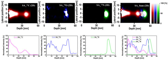
Figure 6.
The 2D (first row) and 1D (second row) profile of the SA output 11C, 15O and 13N radioisotopes and their sum (color in 2D plot corresponds to those in 1D profiles).
The ROIs at which the SA method was applied are schematically illustrated in Figure 4. There are four distinct regions: the whole, edge, plateau and Bragg region (see Figure 4). In Figure 7, the x-axis for all ROIs reflects the extracted half-life of positron emitting radioisotopes (log(2)/β), and the y-axis shows the radionuclide concentration, labeled as normalized α. Considering Figure 7, we observe that for the whole ROI, the contribution from long-lived radioisotopes was dominant. It is observed that the highest contribution from long-lived radioisotopes is for the edge ROI, which is close to 11C radioisotopes. In the plateau region, it is observed that the total contribution is the same as in the whole and edge regions (i.e., the greatest contribution is from long-lived radioisotopes). On the other hand, for the Bragg ROI, the half-life of radioisotopes was slightly larger than that of the 13N radioisotopes. From the present analysis scheme, the activity in the distal fall-off region of proton-induced 13N radioisotopes has been confirmed as the real half-life of 13N is ~10 min. The discretization in SA and measurement errors (background counts and contributions from multiple radioisotopes) would lead to some differences in the estimated half-life value for a specific radioisotope when compared to its known physical half-life.
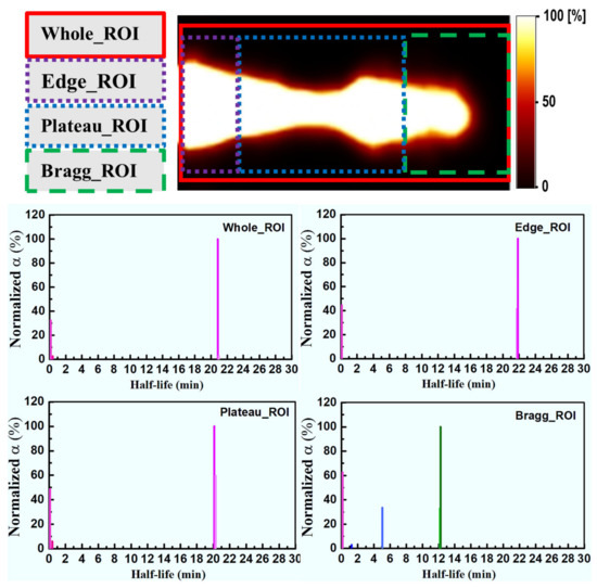
Figure 7.
The spectral analysis (SA) for different ROIs. Pink shows no radioisotope components, magenta shows 11C, blue shows 15O and green shows 13N radioisotopes, respectively.
3.3. The 3D Visualization of Positron Emitting Radioisotopes
For a better visualization, the 3D plots of the spatial distribution of extracted radioisotopes were obtained; these were obtained using the analysis scheme shown in Table 3. The generated 3D distributions and 1D profiles for 11C (shown as SA_11C), 15O (shown as SA_15O) and 13N (shown as SA_13N) radioisotopes are shown in Figure 8. In addition, the simulated dose distribution for an 80 MeV incident proton beam is also shown in Figure 8. The step-by-step procedure and required numerical tools for the preparation of 3D distributions are shown in Table 3. The 3D plots generated from the SA images showed the distinct creation of 11C, 15O and 13N peaks, which could be a promising approach for proton range monitoring and verification. From the 1D profiles shown in Figure 8, the 11C, 15O and 13N peaks were found to be at 33, 39 and 46 mm depths, respectively. Furthermore, the peak of the simulated dose was found to be at 49 mm depth. Therefore, the offset between the simulated dose and the extracted 13N peak was found to be 3 mm.
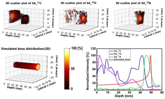
Figure 8.
Three-dimensional scatter visualization and the 1D profiles of 11C, 15O and 13N radioisotopes, along with the simulated dose for the 80 MeV proton beam irradiating water-gel phantom.
4. Discussion
Considering the results shown in Figure 5, two peaks can be observed from the PEMGRAPH measurements. In addition to these two peaks, a small tail peak was observed and vanished rather quickly. The main reason for the formation of these peaks was the proton interaction and scattering from the HDPE container used in the proton irradiation experiment; in particular, the wall effect from the HDPE container that mainly contains carbon (note that 1H nuclei do not produce stable positron emitting radioisotopes). Upon the interaction of proton with matter, the protons lose energy, and hence lower energy protons should be found in the deeper parts of the water-gel phantom, and at shallow depths, there will be more higher energy protons; this satisfies the 11C and 15O threshold energies for their production. The threshold energies for the creation of 11C, 15O and 13N were reported to be 20.61, 16.79 and 5.660 MeV, respectively [41]. As depth increases and in turn the proton energy decreases, the main production reaction is 16O(p,2p2n)13N, which has a lower threshold energy compared to other positron emitting radioisotopes. The current finding using the present scheme is in good agreement with previously reported results [41].
The production of proton-induced radioisotopes was confirmed by the SA approach, which was applied to the dynamic data measured using the PEMGRAPH system. In Figure 6, it was confirmed that the two peaks formed at the entrance (i.e., lower depth) and at the end (i.e., higher depth) were mainly due to the 11C radioisotopes. The 15O peak was formed after the second 11C peak, which is also in agreement with the knowledge of the threshold energy for the production of these radioisotopes and subsequent energy loss of protons at higher depths. Interestingly, the peak of 13N radioisotopes was formed after the 15O peak, mainly due to its lower threshold energy of production; this can be seen in the 1D profile plot shown in Figure 6.
Furthermore, the contribution of proton-induced radioisotopes was confirmed in the ROI study. In Figure 7, the main contributing radioisotopes in the entire edge and plateau regions are shown to be 11C radioisotopes. Considering the Bragg region, the 13N radioisotope makes the highest contribution in the Bragg region. The lowest contribution was found to be from 15O radioisotopes. The SA analysis confirmed the activity in the distal fall-off region of proton-induced 13N radioisotopes. From the 1D profiles in Figure 8, the offset between the simulated dose and extracted 13N peaks is about 3 mm, which is in good agreement with our recent simulation study [42]. Our reported average offset value between the Bragg and the 13N peak was found to be about 2 mm for 80 MeV of incident protons impinging on the water-gel phantom [42]. The present scheme could be applied to inhomogeneous phantoms and small animal experiments after standard irradiation. Further analysis suggests that there is a significant advantage of 3D visualization for proton range verification, especially for inhomogeneous targets (i.e., human organs/tissues).
Considering the generated 3D spatial distribution of positron emitting radioisotopes shown in Figure 8, one can note that the present step-by-step scheme and developed numerical tools can accurately obtain such 3D visualizations. These 3D visualizations would be important when investigating non-uniform targets such as organs in the human body or animal subjects. As shown in Figure 8, 11C radioisotopes formed two peaks at lower depth (near the entrance) and at higher depth (~33 mm). The 15O radioisotopes formed a major peak mainly after 11C radioisotopes and before 13N radioisotopes. The closest peak to the Bragg peak was found to be mainly due to 13N radioisotopes, thanks to their relatively low threshold energy for production. In order to enhance the 3D visualization, the proposed scheme shown in Table 3 was used to generate movie clips for 11C, 15O and 13N radioisotopes, as shown in Figure 8. The movie clips can be downloaded from https://figshare.com/articles/software/An_analysis_scheme_for_3D_visualization_of_positron_emitting_radioisotopes_using_positron_emission_mammography_system/17171093 (accessed on: 11 January 2022).
5. Conclusions
In the present work, a step-by-step analysis scheme using a spectral analysis (SA) approach was introduced. The present scheme determines the 3D spatial distribution of positron emitting radioisotopes, namely 11C, 15O and 13N. All the developed numerical tools that are essential for the present scheme have been made open-source and freely available. The present scheme was tested using proton irradiation experiments and measurements from the PEMGRAPH system. The employed water-gel phantom was irradiated with an 80 MeV monoenergetic pencil-like beam. The results obtained from the present scheme showed the formation of a 13N peak near the Bragg peak, which was found to be in a good agreement with previous investigations. The present scheme and developed tools would be useful for the 3D visualization of positron emitting radioisotopes and in turn for proton range monitoring and verification.
Supplementary Materials
The movie clips, source codes and raw data can be downloaded at: https://figshare.com/articles/software/An_analysis_scheme_for_3D_visualization_of_positron_emitting_radioisotopes_using_positron_emission_mammography_system/17171093.
Author Contributions
Conceptualization, M.R.I. and H.W.; methodology, M.R.I., H.W. and M.S.B.; software, M.S.B. and H.W.; validation, M.R.I., M.S.B., T.Y. and H.W.; formal analysis, M.R.I., M.S.B., S.I., S.G. and H.W.; investigation, M.R.I., M.S.B. and H.W.; resources, S.I., S.G. and H.W.; data curation, M.R.I., M.S.B. and H.W.; writing—original draft preparation, M.R.I.; writing—review and editing, M.S.B. and H.W.; visualization, M.R.I.; supervision, H.W.; project administration, H.W.; funding acquisition, H.W. All authors have read and agreed to the published version of the manuscript.
Funding
This research work was funded by Japan Agency for Medical Research and Development (AMED) under Grant Number 20he2202004h0402 and Ministry of Education, Culture, Sports, Science and Technology (MEXT) under the grant number 21F21103.
Institutional Review Board Statement
All involved institutes were informed about the work done.
Informed Consent Statement
Informed consent is not applicable.
Data Availability Statement
Acknowledgments
The authors thank the Cyclotron and Radioisotopes Center (CYRIC) for the technical support.
Conflicts of Interest
All authors declare that have no conflict of interest.
References
- Shahmohammadi Beni, M.; Krstic, D.; Nikezic, D.; Yu, K.N. A Comparative study on dispersed doses during photon and proton radiation therapy in pediatric applications. PLoS ONE 2021, 16, e0248300. [Google Scholar] [CrossRef] [PubMed]
- Shahmohammadi Beni, M.; Krstic, D.; Nikezic, D.; Yu, K.N. Medium-thickness-dependent proton dosimetry for radiobiological experiments. Sci. Rep. 2019, 9, 11577. [Google Scholar] [CrossRef] [Green Version]
- Shahmohammadi Beni, M.; Ng, C.Y.P.; Krstic, D.; Nikezic, D.; Yu, K.N. Conversion coefficients for determination of dispersed photon dose during radiotherapy: NRUrad input code for MCNP. PLoS ONE 2017, 12, e0174836. [Google Scholar] [CrossRef] [PubMed]
- Shahmohammadi Beni, M.; Krstic, D.; Nikezic, D.; Yu, K.N. Realistic dosimetry for studies on biological responses to X-rays and γ-rays. J. Radiat. Res. 2017, 58, 729–736. [Google Scholar] [CrossRef] [Green Version]
- Nikezic, D.; Shahmohammadi Beni, M.; Krstic, D.; Yu, K.N. Characteristics of protons exiting from a polyethylene converter irradiated by neutrons with energies between 1 KeV and 10 MeV. PLoS ONE 2016, 11, e0157627. [Google Scholar] [CrossRef]
- Knopf, A.C.; Lomax, A. In vivo proton range verification: A review. Phys. Med. Biol. 2013, 58, R131–R160. [Google Scholar] [CrossRef] [PubMed]
- Suit, H.; Urie, M. Proton beams in radiation therapy. J. Natl. Cancer Inst. 1992, 84, 155–164. [Google Scholar] [CrossRef]
- Shahmohammadi Beni, M.; Krstic, D.; Nikezic, D.; Yu, K.N. Modeling kV X-ray-induced coloration in radiochromic films. Appl. Sci. 2018, 8, 106. [Google Scholar] [CrossRef] [Green Version]
- Shahmohammadi Beni, M.; Krstic, D.; Nikezic, D.; Yu, K.N. Modeling coloration of a radiochromic film with molecular dynamics-coupled finite element method. Appl. Sci. 2017, 7, 1031. [Google Scholar] [CrossRef] [Green Version]
- Paganetti, H. Range uncertainties in proton therapy and the role of Monte Carlo simulations. Phys. Med. Biol. 2012, 57, R99–R117. [Google Scholar] [CrossRef]
- Parodi, K.; Polf, J.C. In vivo range verification in particle therapy. Med. Phys. 2018, 16, e1036–e1050. [Google Scholar] [CrossRef] [Green Version]
- Poludniowski, G.; Allinson, N.M.; Evans, P.M. Proton radiography and tomography with application to proton therapy. Br. J. Radiol. 2015, 88, 20150134. [Google Scholar] [CrossRef] [Green Version]
- Hayakawa, Y.; Tada, J.; Arai, N.; Hosono, K.; Sato, M.; Wagai, T.; Tsuji, H.; Tsujii, H. Acoustic pulse generated in a patient during treatment by pulsed proton radiation beam. Radiol. Oncol. Investig. 1995, 3, 42–45. [Google Scholar] [CrossRef]
- Yamaguchi, M.; Torikai, K.; Kawachi, N.; Shimada, H.; Satoh, T.; Nagao, Y.; Fujimaki, S.; Kokubun, M.; Watanabe, S.; Takahashi, T.; et al. Beam range estimation by measuring bremsstrahlung. Phys. Med. Biol. 2012, 57, 2843–2856. [Google Scholar] [CrossRef]
- Min, C.H.; Kim, C.H.; Youn, M.Y.; Kim, J.W. Prompt gamma measurements for locating the dose falloff region in the proton therapy. Appl. Phys. Lett. 2006, 89, 183517. [Google Scholar] [CrossRef]
- Pandey, V.K.; Tan, C.M.; Sangwan, V. GaN-based readout circuit system for reliable prompt gamma imaging in proton therapy. Appl. Sci. 2021, 11, 5606. [Google Scholar] [CrossRef]
- Maccabee, H.D.; Madhvanath, U.; Raju, M.R. Tissue activation studies with alpha-particle beams. Phys. Med. Biol. 1969, 14, 213–224. [Google Scholar] [CrossRef]
- Llacer, J. Positron emission medical measurements with accelerated radioactive ion beams. Nucl. Sci. Appl. 1988, 3, 111–131. [Google Scholar]
- Parodi, K.; Enghardt, W. Potential application of PET in quality assurance of proton therapy. Phys. Med. Biol. 2000, 45, N151–N156. [Google Scholar] [CrossRef] [PubMed]
- Nishio, T.; Miyatake, A.; Inoue, K.; Gomi-Miyagishi, T.; Kohno, R.; Kameoka, S.; Nakagawa, K.; Ogino, T. Experimental verification of proton beam monitoring in a human body by use of activity image of positron-emitting nuclei generated by nuclear fragmentation reaction. Radiol. Phys. Technol. 2008, 1, 44–54. [Google Scholar] [CrossRef]
- Parodi, K.; Ferrari, A.; Sommerer, F.; Paganetti, H. Clinical CT-based calculations of dose and positron emitter distributions in proton therapy using the FLUKA Monte Carlo code. Phys. Med. Biol. 2007, 52, 3369–3387. [Google Scholar] [CrossRef] [PubMed]
- Nishio, T.; Miyatake, A.; Ogino, T.; Nakagawa, K.; Saijo, N.; Esumi, H. The development and clinical use of a beam on-line PET system mounted on a rotating gantry port in proton therapy. Int. J. Radiat. Oncol. Biol. Phys. 2010, 76, 277–286. [Google Scholar] [CrossRef] [PubMed]
- Yamaya, T.; Inaniwa, T.; Minohara, S.; Yoshida, E.; Inadama, N.; Nishikido, F.; Shibuya, K.; Lam, C.F.; Murayama, H. A proposal of an open PET geometry. Phys. Med. Biol. 2008, 53, 757–773. [Google Scholar] [CrossRef]
- Tashima, H.; Yamaya, T.; Yoshida, E.; Kinouchi, S.; Watanabe, M.; Tanaka, E. A single-ring open PET enabling PET imaging during radiotherapy. Phys. Med. Biol. 2012, 57, 4705–4718. [Google Scholar] [CrossRef]
- Enghardt, W.; Debus, J.; Haberer, T.; Hasch, B.G.; Hinz, R.; Jäkel, O.; Krämer, M.; Lauckner, K.; Pawelke, J.; Pönisch, F. Positron emission tomography for quality assurance of cancer therapy with light ion beams. Nucl. Phys. A 1999, 654, 1047c–1050c. [Google Scholar] [CrossRef]
- Vecchio, S.; Attanasi, F.; Belcari, N.; Camarda, M.; Cirrone, G.A.P.; Cuttone, G.; Di Rosa, F.; Lanconelli, N.; Moehrs, S.; Rosso, V.; et al. A PET prototype for “in-beam” monitoring of proton therapy. IEEE Trans. Nucl. Sci. 2009, 56, 51–56. [Google Scholar] [CrossRef]
- Shao, Y.; Sun, X.; Lou, K.; Zhu, X.R.; Mirkovic, D.; Poenisch, F.; Grosshans, D. In-beam PET imaging for on-line adaptive proton therapy: An initial phantom study. Phys. Med. Biol. 2014, 59, 3373–3388. [Google Scholar] [CrossRef] [PubMed]
- Kraan, A.C.; Battistoni, G.; Belcari, N.; Camarlinghi, N.; Cirrone, G.A.P.; Cuttone, G.; Ferretti, S.; Ferrari, A.; Pirrone, G.; Romano, F.; et al. Proton range monitoring with in-beam PET: Monte Carlo activity predictions and comparison with cyclotron data. Phys. Med. 2014, 30, 559–569. [Google Scholar] [CrossRef] [PubMed] [Green Version]
- Sportelli, G.; Belcari, N.; Camarlinghi, N.; Cirrone, G.A.P.; Cuttone, G.; Ferretti, S.; Kraan, A.; Ortuño, J.E.; Romano, F.; Santos, A.; et al. First full-beam PET acquisitions in proton therapy with a modular dual-head dedicated system. Phys. Med. Biol. 2014, 59, 43–60. [Google Scholar] [CrossRef] [PubMed] [Green Version]
- Hsu, D.F.C.; Freese, D.L.; Levin, C.S. Breast-dedicated radionuclide imaging systems. J. Nucl. Med. 2016, 57, 40S–45S. [Google Scholar] [CrossRef] [Green Version]
- Thompson, C.J.; Murthy, K.; Picard, Y.; Weinberg, I.N.; Mako, R. Positron emission mammography (PEM): A promising technique for detecting breast cancer. IEEE Trans. Nucl. Sci. 1995, 42, 1012–1017. [Google Scholar] [CrossRef] [Green Version]
- Abreu, M.C.; Aguiar, J.D.; Almeida, F.G.; Almeida, P.; Bento, P.; Carrico, B.; Ferreira, M.; Ferreira, N.C.; Goncalves, F.; Leong, C.; et al. Design and evaluation of the clear-PEM scanner for positron emission mammography. IEEE Trans. Nucl. Sci. 2006, 53, 71–77. [Google Scholar] [CrossRef]
- Martinez, J.D.; Toledo, J.; Esteve, R.; Mora, F.J.; Sebastia, A.; Benlloch, J.M.; Fernandez, M.; Gimenez, E.N.; Gimenez, M.; Lerche, C.W.; et al. Fully digital trigger and pre-processing electronics for planar positron emission mammography (PEM) scanners. In Proceedings of the IEEE Symposium Conference Record Nuclear Science, Rome, Italy, 16–22 October 2004; IEEE: Manhattan, NY, USA, 2004; pp. 1778–1781. [Google Scholar]
- Huber, J.S.; Choong, W.S.; Wang, J.; Maltz, J.S.; Qi, J.; Mandelli, E.; Moses, W.W. Development of the Lbnl positron emission mammography camera. IEEE Trans. Nucl. Sci. 2003, 50, 1650–1653. [Google Scholar] [CrossRef]
- Wollenweber, S.D.; Williams, R.C.; Beylin, D.; Dolinsky, S.; Weinberg, I.N. Investigation of the quantitative capabilities of a positron emission mammography system. In Proceedings of the IEEE Symposium Conference Record Nuclear Science, Rome, Italy, 16–22 October 2004; pp. 2393–2395. [Google Scholar]
- Miyake, K.K.; Matsumoto, K.; Inoue, M.; Nakamoto, Y.; Kanao, S.; Oishi, T.; Kawase, S.; Kitamura, K.; Yamakawa, Y.; Akazawa, A.; et al. Performance evaluation of a new dedicated breast PET scanner using NEMA NU4-2008 standards. J. Nucl. Med. 2014, 55, 1198–1203. [Google Scholar] [CrossRef] [Green Version]
- Raylman, R.R.; Majewski, S.; Wojcik, R.; Weisenberger, A.G.; Kross, B.; Popov, V.; Schreiman, J.S.; Bishop, H.A. An apparatus for positron emission mammography guided biopsy. In Proceedings of the 1999 IEEE Nuclear Science Symposium, Seattle, WA, USA, 24–30 October 1999; pp. 1323–1327. [Google Scholar]
- Yoshikawa, A.; Yanagida, T.; Kamada, K.; Yokota, Y.; Pejchal, J.; Yamaji, A.; Usuki, Y.; Yamamoto, S.; Miyake, M.; Kumagai, K.; et al. Positron emission mammography using Pr: LuAG scintillator—Fusion of optical material study and systems engineering. Opt. Mater. 2010, 32, 1294–1297. [Google Scholar] [CrossRef]
- Yanagida, T.; Yoshikawa, A.; Yokota, Y.; Kamada, K.; Usuki, Y.; Yamamoto, S.; Miyake, M.; Baba, M.; Kumagai, K.; Sasaki, K.; et al. Development of Pr: LuAG scintillator array and assembly for positron emission mammography. IEEE Trans. Nucl. Sci. 2010, 57, 1492–1495. [Google Scholar] [CrossRef]
- Yanai, A.; Itoh, M.; Hirakawa, H.; Yanai, K.; Tashiro, M.; Harada, R.; Yoshikawa, A.; Yamamoto, S.; Ohuchi, N.; Ishida, T. Newly-developed positron emission mammography (PEM) device for the detection of small breast cancer. Tohoku J. Exp. Med. 2018, 245, 13–19. [Google Scholar] [CrossRef] [Green Version]
- Cho, J.; Grogg, K.; Min, C.H.; Zhu, X.; Paganetti, H.; Lee, H.C.; El Fakhri, G. Feasibility study of using fall-off gradients of early and late pet scans for proton range verification. Med. Phys. 2017, 44, 1734–1746. [Google Scholar] [CrossRef] [PubMed] [Green Version]
- Rafiqul Islam, M.; Shahmohammadi Beni, M.; Ng, C.Y.; Miyake, M.; Rahman, M.; Ito, S.; Gotoh, S.; Yamaya, T.; Watabe, H. Studies on proton range monitoring by utilizing 13N peak for proton therapy applications. PLoS ONE 2021, submitted.
- Shepp, L.A.; Vardi, Y. Maximum likelihood reconstruction for emission tomography. IEEE Trans. Med. Imaging 1982, 1, 113–122. [Google Scholar] [CrossRef] [PubMed]
- Shahmohammadi Beni, M.; Krstic, D.; Nikezic, D.; Yu, K.N. Studies on unfolding energy spectra of neutrons using maximum-likelihood expectation–maximization method. Nucl. Sci. Tech. 2019, 30, 134. [Google Scholar] [CrossRef]
- Carson, R.E.; Huang, S.C.; Phelps, M.E. BLD: A software system for physiological data handling and model analysis. Proc. Annu. Symp. Comput. Appl. Med. Care 1981, 5, 562–565. [Google Scholar]
- Loening, A.M.; Gambhir, S.S. AMIDE: A free software tool for multimodality medical image analysis. Mol. Imaging 2003, 2, 131–137. [Google Scholar] [CrossRef]
- Cunningham, V.J.; Jones, T. Spectral analysis of dynamic PET studies. J. Cereb. Blood Flow Metab. 1993, 13, 15–23. [Google Scholar] [CrossRef] [PubMed]
- Veronese, M.; Rizzo, G.; Bertoldo, A.; Turkheimer, F.E. Spectral analysis of dynamic PET studies: A review of 20 years of method developments and applications. Comput. Math. Methods Med. 2016, 2016, 7187541. [Google Scholar] [CrossRef] [PubMed]
Publisher’s Note: MDPI stays neutral with regard to jurisdictional claims in published maps and institutional affiliations. |
© 2022 by the authors. Licensee MDPI, Basel, Switzerland. This article is an open access article distributed under the terms and conditions of the Creative Commons Attribution (CC BY) license (https://creativecommons.org/licenses/by/4.0/).