Biospeckle Activity of Highbush Blueberry Fruits Infested by Spotted Wing Drosophila (Drosophila suzukii Matsumura)

Abstract

In this study, the potential of the biospeckle phenomenon for detecting fruit infestation by Drosophila suzukii was examined. We tested both graphical and analytical approaches to evaluate biospeckle activity of healthy and infested fruits. As a result of testing the qualitative approach, a generalized difference method proved to be better at identifying infested areas than Fujii’s method. Biospeckle activity of healthy fruits was low and increased with infestation development. It was found that the biospeckle activity index calculated from spatial-temporal speckle correlation of THSP was the best discriminant of healthy fruits and fruits in two different stages of infestation development irrespective of window size and pixel selection strategy adopted to create the THSP. Other numerical indicators of biospeckle activity (inertia moment, absolute value of differences, average differences) distinguished only fruits in later stage of infestation. Regular values of differences turned out to be of no use in detecting infested fruits. We found that to provide a good representation of activity it was necessary to use a strategy aimed at random selection of pixels gathered around the global maximum of biospeckle activity localized on the graphical outcome. The potential of biospeckle analysis for identification of highbush blueberry fruits infested by D. suzukii was confirmed.

1. Introduction

The term biospeckles (or bio-speckles) is often used interchangeably with dynamic speckles [1], boiling speckles [2], dynamic laser speckles or biological laser speckles [3]. Biospeckles (BS) are dynamic patterns appearing as the effect of backscattering of coherent light directed at the surface of biological material. The illuminated surface reflects radiation that differs in phase, thus generating the phenomenon of interference. Consequently, radiation back-scattered from the surface forms an image of spots with an intensity distribution that may change overtime. Non-active samples generate time-invariant images whereas biological samples generate patterns consisting of both time-stable and time-variable speckles [4]. Such patterns may be registered as a movie by means of fast cameras and may be analysed as an image sequence or stack of time-varying images. The dynamics of the biospeckle phenomenon result from the physiological state of the sample, which may vary due to movement of molecules in cells, such as transport of substances across cell membranes or cytoplasm movements [5]. The dependence of biospeckle activity level on sample temperature has also been reported [6]. Due to simplicity of use and great suitability for monitoring subtle changes occurring in biological samples, BS has many applications in agriculture, mainly for pre and post-harvest quality monitoring of agricultural products including detection of damage and diseases [7,8,9,10,11,12,13]. The literature on using BS for detecting fruit infestation by insects is very scarce. Biospeckle imaging is considered a noninvasive technique since up to now no harmful effects of low-power laser light on plant tissues have been reported. Different techniques for measuring biospeckle activity (BA) are generally classified as quantitative or qualitative. The quantitative approach aims to describe the biospeckle activity of the material by means of comprehensive indicators that are calculated from the temporal variability of images (frames) in a sequence. Such indicators use first-order or second-order statistics, ignoring the spatial variation in speckle intensities in consecutive frames, and are often called biospeckle activity indices [14,15] or global measures [16]. On the other hand, the same calculation apparatus may be applied to measure the temporal changes of intensity of each pixel separately, producing a kind of activity map which presents the spatial variation of BA. The former approach is recommended for homogeneous samples, while the latter is considered more appropriate for heterogeneous material wherein spatial variation in biospeckle activity is highly probable [16].

D. suzukii infests mostly in soft fruits such as highbush blueberry, raspberry, blackberry, strawberry, currant, apricot, peach, cherry, plum and even wine grapes [17,18]. Since its first detection in Europe in 2008 (Spain and Italy), this insect has spread extremely quickly across the continent, causing economic losses amounting to millions of US dollars [19]. Estimated revenue losses caused by D. suzukii in strawberry, raspberry, blueberry and blackberry production in 2011–2013 in the Italian province of Trento were around 3 million euros per year (including partial budgeting). The additional costs related to implementation of an integrated control strategy (mass trapping, sanitation, application of insecticides) have been estimated at over 1 million euros per year [20]. Annual costs sustained due to the occurrence of Drosophila suzukii in sweet cherry production areas of Switzerland under four scenarios of increasing fruit infestation ranged between 2000 and 71,000 CHF/ha [21]. Potential losses in peach and fig production in Brazil due to D. suzukii (without considering any control strategy and growers’ adaptation) were estimated at 30 million USD [22]. D. suzukii shows an incredible ability to adapt in various climate conditions. Some adults are cold-tolerant and overwinter successfully to recover from hibernation as soon as temperature exceeds 5 °C. The optimal temperature for development of spotted wing drosophila is 21 °C; therefore, it does well in a temperate climate zone. The insect attacks mainly ripening and undamaged fruit, both wild and cultivated, but females may also inhabit fallen or mechanically damaged fruits (even apples or oranges), as long as it is able to pierce the skin to deposit a clutch of eggs. The oviposition site characterizes with a small scar and with the presence of thin, transparent filaments, which stick out of the scar and are connected with one end of the egg [23]. Such subtle damage may be unnoticed especially if the skin was damaged just before the harvest. The larvae hatch almost immediately after laying the eggs and grow inside the fruit, which causes the scar to soften and collapse after 1–2 days, forming a visible blemish, often accompanied by juice leakage [24]. Currently, there is no effective method of controlling D. suzukii acceptable to both buyers and soft fruit growers, especially those involved in organic farming. So far, growers have used combinations of different methods, ranging from nets and traps for monitoring and mass catching of the pest, through disposal of noncommercial fruit, to chemical treatments. In addition, no effective post-harvest technology has yet been developed for detection of infested fruits harvested because infestation went unnoticed. Such fruits lose their market value but are still a threat to other healthy fruits in storage and transport facilities, and should be removed before placing the harvested fruit in storage.

Since the oviposition site is located just under the fruit’s skin, the presence of eggs or larvae, as well as other accompanying pathogens (bacteria or fungi and the infections they cause) [25], may be the probable biospeckle source. Therefore, we decided to examine the potential of biospeckle phenomenon for detecting fruit infestation by D. suzukii. Specifically, we studied if any tested biospeckle activity measures had the ability to discriminate infested fruits from the healthy fruits. Our goal was to find a biospeckle-based sensor which would be the most responsive towards symptoms, even at an early stage of fruit infestation by D. suzukii, and could be used as a diagnostic tool in post-harvest fruit sorting to avoid the contamination of other fruits in storage. Highbush blueberry fruits were used as an experimental material. Both graphical and analytical approaches were applied to detect the presence of a pest inside the fruit.

2. Materials and Methods

2.1. Material

Material used in this experiment included fruits of highbush blueberry (Vaccinium corymbosum), ‘Darrow’ variety, obtained from a home farm located in north-eastern Poland (52°34′51.6″ N 21°41′04.7″ E). Before starting the experiment, each sample (fruit) was carefully checked for mechanical damage and the presence of pests. Biospeckle images were acquired for twenty randomly chosen, healthy, fully ripe and undamaged fruits as described in Section 2.2. Samples were then placed for 24 h in a rearing container (Figure 1) with fertilized females of spotted wing drosophila.

After this time, fruits were removed from the container and their skins were inspected for traces of piercing by the female ovipositor. A sample was considered to contain eggs if filaments were visible in at least one scar (Figure 2).

At this stage of the experiment only 14 samples were recognized as infested and their biospeckle images were acquired in such a way that at least one oviposition site was facing the camera. After another 48 h (72 h after exposure) it was expected that larvae would be feeding inside the fruits; thus, biospeckle images were acquired again to investigate the biospeckle activity of samples. At this stage, samples were randomly positioned relative to the camera. Acquisition of all image sequences, as well as fruit storage and infestation, were carried out at a room temperature of 21 ± 0.5 °C. Groups of fruits in this experiment were marked as follows: F0—not infested samples (control); F24—infested samples (24 h after exposure); F72—infested samples (72 h after exposure).

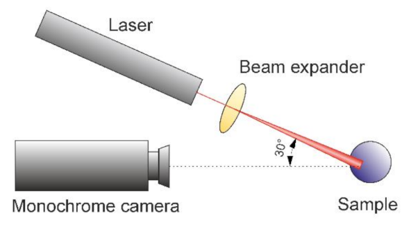
2.2. Experimental Setup

The system for acquisition of biospeckle images is schematically presented in Figure 3.

The system consisted of monochrome camera (model See3CAM_10CUG, USB 3.0, e-con Systems India Pvt Ltd., Guindy, Chennai, India) equipped with a CMOS digital image sensor (model Aptina AR0134, 1/3″, 1.2 Mp, Semiconductor Components Industries, Phoenix, AZ, USA) and CCTV lens (focal length 2.8–12 mm 1/3″, F1.4, LENEX, Poznań, Poland). Samples were illuminated by a He-Ne laser (model 05-LLR-811, Melles Griot IDEX Health & Science, Rochester, NY, USA) of 1 mW power and a wavelength of 632.8 nm. The laser beam was expanded by a microscope objective (PZO, Warsaw, Poland, magnification/aperture 20/0.40). The laser-sample and sample-camera distances were 140 mm and 200 mm, respectively. The experimental setup remained unchanged during the entire study. Samples were placed on a height-adjustable rotary table. Elements of the biospeckle acquisition system (laser, camera, beam expander and rotary table) were mounted on a stable optical bench to eliminate the effect of vibrations from the environment that could disturb the acquisition process. The sample illumination angle was approximately 30 degrees as showed in Figure 3. This angle was established experimentally to avoid the effect of glint from the fruit surface. Biospeckle image sequences were acquired in a dark room to avoid disruptions caused by ambient light. The frame rate was 54 fps and sequences of 256 frames were used for further analysis. The target image resolution, which covered the entire fruit surface lit by by the laser beam was 180 × 180 pixels, which corresponded to an observation area of about 7 × 7 mm.

2.3. Biospeckle Activity Measurement

To analyse biospeckle data, we applied both quantitative and qualitative methods using the Biospeckle Laser Tool Library—BSLTL ver. 1.3.1. [26,27] working on MATLAB 2021a with the Image Processing Toolbox (MathWorks Inc., Natick, MA, USA). In the qualitative approach, we obtained activity maps using the average difference method, known also as Fujii’s method (AD) [16,28,29], and the generalized difference method (GD) [16,29,30].

Fujii’s method consists of creating a map of biospeckle activity by summing the weighted differences between intensities of corresponding pixels in two consecutive images of the sequence, thus preserving information on temporal changes. The Fujii index for each pixel was calculated from Equation (1) [16]:

$$F\left(x,y\right) = {{\displaystyle \sum }}_{k = 1}^N\frac{\left|I_k\left(x,y\right) - I_{k + 1}\left(x,y\right)\right|}{I_k\left(x,y\right) + I_{k + 1}\left(x,y\right)}$$

(1)

The generalized difference method is an alternative to AD but does not include normalization. Each value of the GD map corresponds to the cumulative sum of differences in single pixel intensity calculated between each image and all other images in the sequence, which is represented by Equation (2) [16].

$$GD\left(x,y\right) = {{\displaystyle \sum }}_{k = 1}^{N - 1}{{\displaystyle \sum }}_{l = k + 1}^N\left|I_k\left(x,y\right) - I_l\left(x,y\right)\right|$$

(2)

In Equations (1) and (2) k = 1,2, … N stands for image index in the image sequence and I_k is the intensity of pixel with x,y coordinates. Activity maps generated by AD and GD were obtained using functions fujii() and gendiff() respectively.

The quantitative approach to evaluate biospeckle activity was realised by creating time history speckle patterns (THSPs). A THSP was formed by chronologically arranging the same column taken from each image in the sequence. Consequently, changes in pixel intensity over time were shown in the horizontal direction, while spatial changes were shown in the vertical direction [1]. On this basis, a second order histogram, i.e., co-occurrence matrix (COM) was calculated to represent the frequency of changes in pixel intensities over time. Each COM value corresponded to the number of pairs of pixels with intensity i and j that appeared in the THSP image, one after another, in the direction of 0° (time lapse) [7,31,32]. Normalisation of COM leads to reduction of image heterogeneity by making the sum of all values equal to one, according to Equation (3) [32].

$$NCO{M}_{ij} = \frac{CO{M}_{ij}}{{\sum }_{ij}CO{M}_{ij}}$$

(3)

where COM_ij stands for the value in a row i and a column j of the co-occurrence matrix.

NCOM was the basis to calculate other biospeckle activity indices, such as inertia moment (IM), absolute values of differences (AVD), regular value of differences (RVD) and average differences (obtained by numerical analysis) (NAD) [1,2,33,34].

The inertia moment corresponds to dispersion of NCOM values around the principal diagonal and was calculated by Equation (4) [1]:

$$IM = {{\displaystyle \sum }}_{i,j}NCO{M}_{ij}{\left|j - i\right|}^2$$

(4)

The higher the IM values, the stronger the biospeckle activity. Nonetheless, a square operation may result in distortion of variations that occur in THSP; therefore, absolute value of differences were calculated by Equation (5) [33]:

$$AVD = {{\displaystyle \sum }}_{i,j}NCO{M}_{ij}\left|j - i\right|$$

(5)

The regular value of differences is similar to AVD but substitutes absolute value of differences with the ordinary difference that occurs between two consecutive pixels, as follows (6) [26]:

$$RVD = {{\displaystyle \sum }}_{i,j}NCO{M}_{ij}\left(j - i\right)$$

(6)

The numerical version of AD proposed by Reis et al. [34] measures mean relative contrast between intensities of consecutive images, and was calculated by Equation (7):

$$NUMAD = {{\displaystyle \sum }}_{i,j}NCO{M}_{ij}\frac{\left|i - j\right|}{\left(i + j\right)}$$

(7)

In addition, correlation of THSP (TCORR) was obtained from Formula (8) given by Xu et al. [35]:

$$TCOR{R}_j = \frac{1}{N/2}{{\displaystyle \sum }}_{i = 1}^{N/2}\frac{{\sum }_{k = 1}^N{I}_{k,i} · I_{k,i + j}}{\sqrt{{\sum }_{k = 1}^N{\left(I_{k,i}\right)}^2 · {\sum }_{k = 1}^N{\left(I_{k,i + j}\right)}^2}}$$

(8)

Functions thsp2corr(), coom(), inertiamoment(), avd(), rvd() and numad() available in BSLTL were used to calculate TCORR, NCOM, IM, AVD, RVD and NAD respectively. On the basis of TCORR values, the biospeckle activity indicator (BAI) was calculated according to the Equation (9) [9,36]:

$$BAI = 1 - TCORR$$

(9)

We also tested a few strategies of creating THSP. The creation of THSPs was preceded by analysis of activity maps and identification of regions with high and homogeneous biospeckle activity. We used the homogeneity() function to create both a matrix of homogeneity percentages based on IM as an activity indicator, and a map of spatial distribution of IM means, each one calculated in 5 × 5-pixel windows. Once we found the global maxima of activity in analysed sequences we used them to establish a region of interest (ROI) with dimensions of 51 × 51 with the maximum in the centre and create THSPs in two different ways. First we used the method proposed by Oulamara et al. [37], which consisted of extracting the same column of pixels from each frame in a sequence and placing them side by side in a chronological order. In our study the selected column contained a pixel identified as belonging to the global maximum of BA and we used the thsp() function to create THSP. In this approach, we tested whole ROI with dimensions of 51 × 51, as well as smaller ROIs with dimensions of 5 × 5, 9 × 9, 13 × 13, 17 × 17, 21 × 21 and 25 × 25 pixels. In the second method, we extracted from ROI a set of random points using a Gaussian distribution and arranged them as they followed one after another in time [38]. The ROI for 50 random points selection contained the global maximum of BA in its centre and had dimensions of 31 × 31 pixels. The function to create THSP in this way was thsp_gaussian().

2.4. Statistical Analysis

The experiment was carried out in three stages. At each stage, biospeckle images were acquired for different regions of the same sample. As a result, we obtained biospeckle activity for three independent groups. Shapiro-Wilk’s test for normality, as well as Levene’s test for homogeneity of variance in groups, indicated that global measures of biospeckle activity in this experiment did not meet the assumptions for classical one-way ANOVA. Therefore, the Kruskal-Wallis test by ranks was used to analyse groups for stochastic dominance. The Kruskal-Wallis multiple test was then applied to analyse differences between mean ranks for each pair of groups. Differences were considered to be significant at p-value ≤ 0.05. Skewness was calculated according to Equation (10).

$$Skew. = \frac{n{\sum }_i{\left(x_i - \overline{x}\right)}^3}{\left(n - 1\right)\left(n - 2\right)s^3}$$

(10)

where n denotes sample size, x_i stands for ith observation, $\overline{x}$ is the arithmetic mean and s denotes sample standard deviation. Statistical analyses were performed using Statistica, version 13.3 software (TIBCO Software Inc., Palo Alto, CA, USA, 2017).

3. Results and Discussion

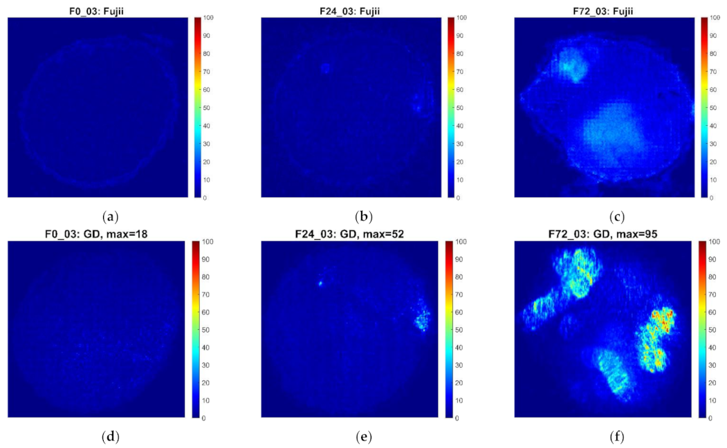
3.1. Qualitative Description of Biospeckle Activity

The example graphical outcomes obtained by the AD and GD methods is presented in Figure 4. The dark blue colour represents regions with low BA, whereas the dark red colour corresponds to the highest BA. Images show the whole area illuminated by the laser, so circular boundaries of the beam may be noticeable. In the late stage of infestation, fruits started to deform; thus the irregular shape of the illuminated region. The left column of Figure 4 contains activity maps of the uninfested sample. Results obtained by both methods clearly indicated that the tested fruits had very low biospeckle activity. Highbush blueberry is a climacteric fruit, which means that after harvesting, processes related to respiration and transpiration take place, but its rate of ethylene production was much lower than in other typical climacteric fruits, e.g., apples, with activity maps showing higher values [16]. The middle column in Figure 4 shows activity maps of a fruit with visible signs of puncture on its skin.

Since fruits were positioned with scar or scars facing the camera lens, it would be expected that the oviposition site, or its near location, would show a different (higher) biospeckle activity, because scars are often attacked by other pathogens, most often fungi. Activity maps obtained by the GD method revealed regions wherein biospeckle activity slightly increased. An example map in Figure 4e contains two brighter areas, one on the upper left side of the fruit and the other slightly lower on the right edge of the illuminated area. On activity maps generated by Fujii’s method, these areas were not visible or were barely visible, as shown in Figure 4b. The rightmost column of Figure 4 presents biospeckle activity of a sample inspected 48 h after removing it from the rearing container. By this time, larvae started feeding inside the flesh, and skin at the puncture site collapsed. Results obtained with the Fujii’s method contained areas of increased activity, which were a little more visible than in the previous phase. Their contours, however, appeared blurred as shown in Figure 4c. Such a result may indicate that the dynamics of intensity transitions were low. Fujii’s method analyses only consecutive frames in the sequence, which provides temporal information [28,29]; thus, the low frequency of changes resulted in poor representation on the activity map. This effect may also be related to the frame rate being too high in relation to the frequency of speckle intensity changes. Activity maps generated by the GD method resulted in much better contours of regions of heightened biospeckle activity and, in some cases, pipe-like shapes occurred as shown in Figure 4f. Given previous considerations, as well as the shape of the active areas discovered by the GD method, it cannot be ruled out that not only destruction of the fruit flesh caused by the larvae feeding may be the source of BA, but also the larvae themselves. Better representation of BA by GD outcomes results from a different calculation protocol that incorporates intensity differences between all frames including nonconsecutive ones [16]. Since analysis of BA of highbush blueberry aim mostly at detection of a pest, the information about the temporal variability in pixel brightness is ultimately less essential. Therefore, the GD method may prove more useful for detecting BA especially if it is not uniform within the investigated area [39], as for samples from F24 or F72 series.

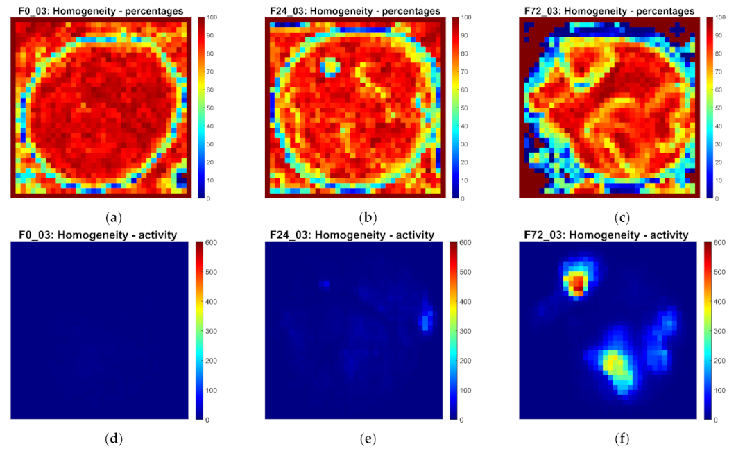
3.2. Spatial Homogeneity of Biospeckle Activity

Graphical outcomes of homogeneity in BA in analysed groups of samples are presented in Figure 5a–c, and maps of spatial variability of IM are presented in Figure 5d–f. Graphical representation of biospeckle activity is very useful, but from a practical point of view quantitative measures are more desirable for ease of interpretation. For this reason, we decided to carry out the homogeneity test using inertia moment as an activity indicator to localize regions homogeneous enough to establish ROI for further analysis. As expected, regions of highest homogeneity of BA, as well as the lowest values of IM, were observed in uninfested samples (Figure 5a,d). As for samples of the F24 (Figure 5b) and F72 (Figure 5c) series, homogeneity decreased with increasing area of the higher IM indicator. Due to the local nature of occurrence of potential biospeckle activity sources, we decided to localize ROIs around the global maxima contained in areas with the highest IM values, taking into account information on homogeneity to avoid the analysis of transition areas.

3.3. Quantitative Analysis of Biospeckle Activity

Arithmetic means and medians of BA indices for an ROI of 51 × 51 pixels, calculated for the THSP obtained from a single column, are presented in

Table 1. Basic statistics calculated for THSP obtained from single column of ROI of 51 × 51 pixels with the global maximum at the central point.

Activity Indicator	F0			F24			F72
	Mean	Median	Mean Rank	Mean	Median	Mean Rank	Mean	Median	Mean Rank
AVD	0.994	0.917	14.000 a	1.445	1.165	18.733 a	4.122	2.720	36.267 b
IM	3.848	2.943	12.667 a	13.263	4.614	20.067 a	98.974	37.922	36.267 b
RVD	−0.002	−0.002	24.733 a	−0.001	−0.002	24.000 a	−0.004	−0.007	20.267 a
NAD	0.009	0.009	13.133 a	0.012	0.010	18.600 a	0.033	0.027	37.267 b
BAI	0.003	0.003	9.133 a	0.014	0.013	22.333 b	0.075	0.070	37.533 c

F0—uninfested samples (control); F24—infested samples (24 h after exposure); F72—infested samples (72 h after exposure); IM—inertia moment; AVD—average value of differences; RVD—regular value of differences; NAD—average difference; BAI—biospeckle activity indicator. ^a–c different lower-case letters in the same row indicate significantly different values of mean ranks (p ≤ 0.05).

.

Analysing means in F0, F24 and F72 groups, it may be noticed that IM and BAI had the greatest discrimination potential because their values differed the most between groups. The highest disproportions between groups were observed for means and medians of the IM indicator.

The IM mean in the F24 group was 3.35 times higher than in the F0 group, whereas the mean calculated for F72 exceeded it more than seven times, and being higher than the mean in group F0 by about 25 times. Similar means proportions were observed for the BAI indicator which was more than 23 times lower in F0 and five times lower in the F24 group compared to the F72 group. AVD means, as well as NAD means, were not so varied, whereas mean value of RVD had the lowest variation between groups. Taking into account the mechanism of calculating IM as the squared distance from the NCOM diagonal, it was not a good measure of BA in the case of regions with heterogeneous activity, as in our experiment. It should be also noted that in F24 and F72 stages, high disproportions between means and medians of some parameters were observed, which is probably the effect of differentiation between biological samples. Nonetheless, this fact may definitely affect numerical analysis, especially evaluation of differences between groups. As may be noticed, differences between means and medians of IM proved to be considerable, indicating a strong skewness which was of 1.6, 3.36 and 2.78 in the F0, F24 and F72 groups, respectively. High skewness was also observed for the AVD indicator (2.93 and 1.7 in F24 and F72 group, respectively) as well as for the NAD variable within the F24 group. For this reason, homogeneity of variances in groups was tested, which in each case resulted in rejection of the hypothesis concerning their equality. Therefore, significance of differences between groups was tested using the non-parametric Kruskal-Wallis test for ranks. Results showed no significant differences between groups in terms of RVD values. As for AVD, IM and NAD, differences were significant only between F24–F72 and F0–F72 group pairs, as marked in Table 1. The only variable with values significantly different in all groups was BAI, based on correlation with THSP. Similar to the GD method with correlation of THSP, BAI considers non-consecutive frames in an image sequence, and is more sensitive to subtle and local changes of BA levels, being robust to incidental noise in the spatial domain at the same time.

Taking into account sensitivity to heterogeneity of activity areas observed in the case of IM, we decided to check BA indicators in terms of their ability to discriminate between groups of fruits depending on ROI size. Basic statistics for tested BA indicators calculated from THSP obtained from a single column of different sizes are shown in

Table 2. Basic statistics for biospeckle indices calculated for THSP obtained from a single column extracted from ROIs of dimensions ranging from 5 × 5 to 25 × 25 pixels with the global maximum in the central point.

Activity Indicator	F0			F24			F72
	Mean	Median	Mean Rank	Mean	Median	Mean Rank	Mean	Median	Mean Rank
ROI of 5 × 5 pixels
AVD	2.100	2.056	12.571 a	3.193	2.347	18.286 a	10.614	6.491	33.643 b
IM	12.306	8.422	12.357 a	34.804	12.913	18.786 a	430.228	96.285	33.357 b
RVD	−0.028	−0.020	21.071 a	0.009	−0.055	20.929 a	0.011	−0.004	22.500 a
NAD	0.010	0.009	13.000 a	0.013	0.011	17.714 a	0.043	0.030	33.786 b
BAI	0.008	0.005	9.429 a	0.025	0.026	19.929 b	0.072	0.068	35.143 c
ROI of 9 × 9 pixels
AVD	1.947	2.024	12.643 a	2.987	2.268	18.143 a	9.821	6.241	33.714 b
IM	10.312	8.197	12.286 a	30.042	12.390	18.714 a	358.510	87.934	33.500 b
RVD	−0.018	−0.004	20.214 a	0.010	−0.024	21.000 a	0.026	0.008	23.286 a
NAD	0.010	0.009	12.929 a	0.014	0.012	17.857 a	0.043	0.033	33.714 b
BAI	0.008	0.005	9.143 a	0.023	0.019	20.071 b	0.081	0.075	35.286 c
ROI of 13 × 13 pixels
AVD	1.904	1.942	12.643 a	2.896	2.314	18.071 a	9.267	6.156	33.786 b
IM	9.805	7.743	12.286 a	29.655	12.710	18.500 a	320.123	84.297	33.714 b
RVD	−0.016	−0.006	19.571 a	0.009	−0.012	21.571 a	0.023	0.003	23.357 a
NAD	0.010	0.010	12.786 a	0.014	0.011	18.143 a	0.043	0.035	33.571 b
BAI	0.007	0.005	9.214 a	0.021	0.019	20.071 b	0.080	0.079	35.214 c
ROI of 17 × 17 pixels
AVD	1.832	1.884	12.429 a	2.829	2.382	18.071 a	8.936	6.000	34.000 b
IM	9.100	7.370	12.071 a	28.217	13.226	18.714 a	299.208	81.160	33.714 b
RVD	−0.013	−0.010	19.286 a	−0.003	−0.014	21.214 a	0.017	0.007	24.000 a
NAD	0.010	0.010	12.000 a	0.015	0.012	19.000 a	0.043	0.036	33.500 b
BAI	0.007	0.004	9.429 a	0.019	0.016	19.571 b	0.081	0.078	35.500 c
ROI of 21 × 21 pixels
AVD	1.796	1.832	12.429 a	2.802	2.460	18.214 a	8.515	5.854	33.857 b
IM	8.768	7.012	12.000 a	30.337	13.852	18.571 a	272.390	77.266	33.929 b
RVD	−0.008	−0.003	19.429 a	−0.006	−0.011	18.714 a	0.019	0.018	26.357 a
NAD	0.010	0.009	12.071 a	0.015	0.012	18.857 a	0.043	0.036	33.571 b
BAI	0.007	0.004	9.286 a	0.019	0.016	19.714 b	0.082	0.076	35.500 c
ROI of 25 × 25 pixels
AVD	1.782	1.792	12.500 a	2.743	2.474	18.214 a	8.265	5.757	33.786 b
IM	8.624	6.774	11.929 a	29.851	13.605	18.714 a	258.270	73.311	33.857 b
RVD	−0.008	−0.005	19.929 a	−0.007	−0.011	19.286 a	0.015	0.020	25.286 a
NAD	0.010	0.009	12.000 a	0.015	0.012	19.000 a	0.043	0.036	33.500 b
BAI	0.006	0.004	9.143 a	0.018	0.015	19.857 b	0.080	0.072	35.500 c

F0—uninfested samples (control); F24—infested samples (24 h after exposure); F72—infested samples (72 h after exposure); IM—inertia moment; AVD—average value of differences; RVD—regular value of differences; NAD—average difference; BA—biospeckle activity. ^a–c different lower-case letters in the same row indicate significantly different values of mean ranks (p ≤ 0.05).

.

Comparing results of the Kruskal-Wallis multiple test for mean ranks, identical effects were obtained in each ROI size. RVD did not prove successful as a measure of activity differentiation of infested and uninfested fruits. AVD, IM and NAD showed the potential to distinguish only the late stage of infestation. As previously described, BAI turned out to be the best discriminant of healthy, early and late stage of infestation. As for results obtained for IM in different ROI, its values in groups were considerably different as observed earlier, which proves that BA changed drastically with infestation development (from F0 to F72). This observation confirms the high sensitivity of this indicator to the presence of disruptions in pixel intensities [40], and at the same time indicates local changes in biospeckle activity of fruits. Due to the specificity of this phenomenon, the inertia moment is not a good indicator of infestation.

As an alternative to extraction of a single line or column from consecutive frames, THSP may be created by a pixel collection randomly selected from a window of fixed size. In our study we adopted the strategy of selection of pixels with values following a Gaussian distribution. Further, the same quantitative measures used previously were calculated.

Table 3. Basic statistics for biospeckle indices calculated for THSP obtained from a random set of points follow a Gaussian distribution.

Activity Indicator	F0			F24			F72
	Mean	Median	Mean Rank	Mean	Median	Mean Rank	Mean	Median	Mean Rank
AVD	1.776	1.906	14.400 a	2.534	2.152	18.333 a	8.421	5.660	36.267 b
IM	8.260	7.496	13.400 a	24.279	12.010	19.267 a	272.559	77.261	36.333 b
RVD	−0.004	−0.003	26.800 a	0.001	−0.005	21.533 a	0.013	0.006	20.667 a
NAD	0.010	0.010	12.933 a	0.015	0.011	20.533 a	0.041	0.033	35.533 b
BAI	0.004	0.003	9.467 a	0.014	0.014	22.267 b	0.076	0.071	37.267 c

F0—uninfested samples (control); F24—infested samples (24 h after exposure); F72—infested samples (72 h after exposure); IM—inertia moment; AVD—average value of differences; RVD—regular value of differences; NAD—average difference; BA—biospeckle activity. ^a–c different lower-case letters in the same row indicate significantly different values of mean ranks (p ≤ 0.05).

presents means, medians and effects of mean ranks comparison for BA indices calculated from THSP built in such a way.

Indicators AVD and IM had lower values in comparison to those from Table 1, whereas NAD, RVD and BAI were slightly different. As observed in earlier analyses, the RVD indicator did not differ significantly between groups, so this index is not appropriate for identification of infested fruits. As might be expected, indices IM, AVD and NAD did not distinguish fruits in early stage of infestation from healthy ones. The only indicator which differed significantly in all groups was BAI. Slight differences between BAI means and medians in groups prove its robustness to outliers and extremes. A similar indicator of BA employing the Pearson correlation coefficient, was proposed by other researchers as a reliable measure suitable for monitoring the quality of fresh and stored fruits [36,41,42,43,44]. Although results obtained in this and other analyses are similar, random selection of pixels seems to be a better solution if analysing regions heterogeneous in terms of BA; hence, THSP created in this way should be more representative for such regions.

4. Conclusions

The biospeckle activity of healthy and infested fruits was found to be different as shown by graphical and numerical results of activity analyses. Activity of healthy fruits was low and increased with infestation development, but spatial distribution of oviposition sites, which were the source of biospeckle activity, made numerical analysis difficult. Regions punctured by the ovipositor showed higher activity than those that were not infested; thus, heterogeneity of intensities occurred with local peaks of activity spatially distributed in the biospeckle image. As a result of testing a qualitative approach to analyse biospeckle activity, it turned out that the GD method worked well in identifying infested areas. Out of numerical indicators of biospeckle activity calculated on the basis of the THSP image, only the biospeckle activity index, and correlation with THSP, proved to distinguish healthy fruits from those in the early stage of infestation. To provide a good representation of activity it is advisable to use a strategy aimed at random selection of pixels gathered around the global maximum of biospeckle activity or, if it is required, around a few local maxima. The potential of laser speckle analysis as a method for identification of highbush blueberry fruits infested by D. suzukii was confirmed.

Further studies should be conducted to improve the activity measurement protocol and search for technical solutions enabling application of biospeckle analysis in automation of the pest identification process at the post-harvest stage.

References

1. Arizaga, R.; Trivi, M.; Rabal, H. Speckle Time Evolution Characterization by the Co-Occurrence Matrix Analysis. Opt. Laser Technol. 1999, 31, 163–169. [Google Scholar] [CrossRef]
2. Ansari, M.Z.; Nirala, A.K. Assessment of Bio-Activity Using the Methods of Inertia Moment and Absolute Value of the Differences. Optik 2013, 124, 512–516. [Google Scholar] [CrossRef]
3. Catalano, M.D.; Rivera, F.P.; Braga, R.A. Viability of Biospeckle Laser in Mobile Devices. Optik 2019, 183, 897–905. [Google Scholar] [CrossRef]
4. Briers, J.D. Wavelength Dependence of Intensity Fluctuations in Laser Speckle Patterns from Biological Specimens. Opt. Commun. 1975, 13, 324–326. [Google Scholar] [CrossRef]
5. Braga, R.A.; Dupuy, L.; Pasqual, M.; Cardoso, R.R. Live Biospeckle Laser Imaging of Root Tissues. Eur. Biophys. J. 2009, 38, 679–686. [Google Scholar] [CrossRef]
6. Kurenda, A.; Adamiak, A.; Zdunek, A. Temperature Effect on Apple Biospeckle Activity Evaluated with Different Indices. Postharvest Biol. Technol. 2012, 67, 118–123. [Google Scholar] [CrossRef]
7. Pajuelo, M.; Baldwin, G.; Rabal, H.; Cap, N.; Arizaga, R.; Trivi, M. Bio-Speckle Assessment of Bruising in Fruits. Opt. Lasers Eng. 2003, 40, 13–24. [Google Scholar] [CrossRef]
8. Rabelo, G.F.; Enes, A.M.; Braga Junior, R.A.; Dal Fabbro, I.M. Frequency Response of Biospeckle Laser Images of Bean Seeds Contaminated by Fungi. Biosyst. Eng. 2011, 110, 297–301. [Google Scholar] [CrossRef]
9. Adamiak, A.; Zdunek, A.; Kurenda, A.; Rutkowski, K. Application of the Biospeckle Method for Monitoring Bull’s Eye Rot Development and Quality Changes of Apples Subjected to Various Storage Methods—Preliminary Studies. Sensors 2012, 12, 3215–3227. [Google Scholar] [CrossRef] [PubMed]
10. Enes, A.M.; Fracarolli, J.A.; Fabbro, I.M.D.; Rodrigues, S. Biospeckle Supported Fruit Bruise Detection. Int. J. Nutr. Food Eng. 2012, 6, 889–891. [Google Scholar]
11. Sutton, D.B.; Punja, Z.K. Investigating Biospeckle Laser Analysis as a Diagnostic Method to Assess Sprouting Damage in Wheat Seeds. Comput. Electron. Agric. 2017, 141, 238–247. [Google Scholar] [CrossRef]
12. Gao, Y.; Rao, X. Blackspot Bruise in Potatoes: Susceptibility and Biospeckle Activity Response Analysis. J. Food Meas. Charact. 2019, 13, 444–453. [Google Scholar] [CrossRef]
13. Wu, A.; Zhu, J.; Ren, T. Detection of Apple Defect Using Laser-Induced Light Backscattering Imaging and Convolutional Neural Network. Comput. Electr. Eng. 2020, 81, 106454. [Google Scholar] [CrossRef]
14. Alves, R.A.; Oliveira Silva, B.; Rabelo, G.; Marques Costa, R.; Machado Enes, A.; Cap, N.; Rabal, H.; Arizaga, R.; Trivi, M.; Horgan, G. Reliability of Biospeckle Image Analysis. Opt. Lasers Eng. 2007, 45, 390–395. [Google Scholar] [CrossRef]
15. Amaral, I.C.; Braga, R.A.; Ramos, E.M.; Ramos, A.L.S.; Roxael, E.A.R. Application of Biospeckle Laser Technique for Determining Biological Phenomena Related to Beef Aging. J. Food Eng. 2013, 119, 135–139. [Google Scholar] [CrossRef] [Green Version]
16. Zdunek, A.; Adamiak, A.; Pieczywek, P.M.; Kurenda, A. The Biospeckle Method for the Investigation of Agricultural Crops: A Review. Opt. Lasers Eng. 2014, 52, 276–285. [Google Scholar] [CrossRef]
17. Bellamy, D.E.; Sisterson, M.S.; Walse, S.S. Quantifying Host Potentials: Indexing Postharvest Fresh Fruits for Spotted Wing Drosophila, Drosophila Suzukii. PLoS ONE 2013, 8, e61227. [Google Scholar] [CrossRef] [Green Version]
18. Ioriatti, C.; Walton, V.; Dalton, D.; Anfora, G.; Grassi, A.; Maistri, S.; Mazzoni, V. Drosophila Suzukii (Diptera: Drosophilidae) and Its Potential Impact to Wine Grapes During Harvest in Two Cool Climate Wine Grape Production Regions. J. Econ. Entomol. 2015, 108, 1148–1155. [Google Scholar] [CrossRef] [PubMed] [Green Version]
19. De Ros, G.; Grassi, A.; Pantezzi, T. Recent Trends in the Economic Impact of Drosophila suzukii. In Drosophila suzukii Management; Garcia, F.R.M., Ed.; Springer: Cham, Switzerland, 2020; ISBN 9783030626914. [Google Scholar] [CrossRef]
20. De Ros, G.; Concia, S.; Pantezzia, T.; Savinib, G. The economic impact of invasive pest Drosophila suzukii on berry production in the Province of Trento, Italy. J. Berry Res. 2015, 5, 89–96. [Google Scholar] [CrossRef] [Green Version]
21. Mazzi, D.; Bravin, E.; Meraner, M.; Finger, R.; Kuske, S. Economic Impact of the Introduction and Establishment of Drosophila suzukii on Sweet Cherry Production in Switzerland. Insects 2017, 8, 18. [Google Scholar] [CrossRef] [PubMed] [Green Version]
22. Benito, N.P.; Lopes-da-Silva, L.; Sivori Silva dos Santos, R. Potential spread and economic impact of invasive Drosophila suzukii in Brazil. Pesqui. Agropecuária Bras. 2016, 51, 571–578. [Google Scholar] [CrossRef] [Green Version]
23. Walsh, D.B.; Bolda, M.P.; Goodhue, R.E.; Dreves, A.J.; Lee, J.; Bruck, D.J.; Walton, V.M.; O’Neal, S.D.; Zalom, F.G. Drosophila Suzukii (Diptera: Drosophilidae): Invasive Pest of Ripening Soft Fruit Expanding Its Geographic Range and Damage Potential. J. Integr. Pest Manag. 2011, 2, G1–G7. [Google Scholar] [CrossRef]
24. Grassi, A.; Giongo, L.; Palmieri, L. Drosophila (Sophophora) Suzukii (Matsumura), New Pest of Soft Fruits in Trentino (North-Italy) and in Europe. IOBC/WPRS Bull. 2011, 70, 121–128. [Google Scholar]
25. Ioriatti, C.; Guzzon, R.; Anfora, G.; Ghidoni, F.; Mazzoni, V.; Villegas, T.R.; Dalton, D.T.; Walton, V.M. Drosophila Suzukii (Diptera: Drosophilidae) Contributes to the Development of Sour Rot in Grape. J. Econ. Entomol. 2018, 111, 283–292. [Google Scholar] [CrossRef] [PubMed]
26. Braga, R.A.; Rivera, F.P. Junio Moreira A Practical Guide to Biospeckle Laser Analysis: Theory and Software; Editora UFLA: Lavras, Brazil, 2016; ISBN 9788581270517. [Google Scholar]
27. Bio-Speckle Laser Tool Library. Available online: http://www.nongnu.org/bsltl/ (accessed on 20 October 2021).
28. Fujii, H.; Nohira, K.; Yamamoto, Y.; Ikawa, H.; Ohura, T. Evaluation of Blood Flow by Laser Speckle Image Sensing. Part 1. Appl. Opt. 1987, 26, 5321–5325. [Google Scholar] [CrossRef]
29. Pandiselvam, R.; Mayookha, V.P.; Kothakota, A.; Ramesh, S.V.; Thirumdas, R.; Juvvi, P. Biospeckle Laser Technique—A Novel Non-Destructive Approach for Food Quality and Safety Detection. Trends Food Sci. Technol. 2020, 97, 1–13. [Google Scholar] [CrossRef]
30. Arizaga, R.A.; Cap, N.L.; Rabal, H.J.; Trivi, M. Display of Local Activity Using Dynamical Speckle Patterns. Opt. Eng. 2002, 41, 287–294. [Google Scholar] [CrossRef]
31. Haralick, R.M.; Shanmugam, K.; Dinstein, I. Textural Features for Image Classification. IEEE Trans. Syst. Man Cybern. 1973, SMC-3, 610–621. [Google Scholar] [CrossRef] [Green Version]
32. Cardoso, R.R.; Braga, R.A. Enhancement of the Robustness on Dynamic Speckle Laser Numerical Analysis. Opt. Lasers Eng. 2014, 63, 19–24. [Google Scholar] [CrossRef]
33. Braga, R.A.; Nobre, C.M.B.; Costa, A.G.; Sáfadi, T.; da Costa, F.M. Evaluation of Activity through Dynamic Laser Speckle Using the Absolute Value of the Differences. Opt. Commun. 2011, 284, 646–650. [Google Scholar] [CrossRef]
34. Reis, R.O.; Rabal, H.J.; Braga, R.A. Light Intensity Independence during Dynamic Laser Speckle Analysis. Opt. Commun. 2016, 366, 185–193. [Google Scholar] [CrossRef]
35. Xu, Z.; Joenathan, C.; Khorana, B.M. Temporal and Spatial Properties of the Time-Varying Speckles of Botanical Specimens. Opt. Eng. 1995, 34, 1487–1502. [Google Scholar] [CrossRef]
36. Ansari, M.D.Z.; Nirala, A.K. Biospeckle Activity Measurement of Indian Fruits Using the Methods of Cross-Correlation and Inertia Moments. Optik 2013, 124, 2180–2186. [Google Scholar] [CrossRef]
37. Oulamara, A.; Tribillon, G.; Duvernoy, J. Biological Activity Measurement on Botanical Specimen Surfaces Using a Temporal Decorrelation Effect of Laser Speckle. J. Mod. Opt. 1989, 36, 165–179. [Google Scholar] [CrossRef]
38. Papoulis, A.; Pillai, S.U. Probability, Random Variables, and Stochastic Processes; McGraw-Hill: New York, NY, USA, 1984; ISBN 9780070486584. [Google Scholar]
39. Braga, R.A.; Dal Fabbro, I.M.; Borem, F.M.; Rabelo, G.; Arizaga, R.; Rabal, H.J.; Trivi, M. Assessment of Seed Viability by Laser Speckle Techniques. Biosyst. Eng. 2003, 86, 287–294. [Google Scholar] [CrossRef] [Green Version]
40. Braga, R.; Cardoso, R.R.; Bezerra, P., Jr.; Wouters, F.; Sampaio, G.; Varaschin, M. Biospeckle Numerical Values over Spectral Image Maps of Activity. Opt. Commun. 2012, 285, 553–561. [Google Scholar] [CrossRef]
41. Zdunek, A.; Muravsky, L.I.; Frankevych, L.; Konstankiewicz, K. New Nondestructive Method Based on Spatial-Temporal Speckle Correlation Technique for Evaluation of Apples Quality during Shelf-Life. Int. Agrophys. 2007, 21, 305–310. [Google Scholar]
42. Ansari, M.Z.; Minz, P.D.; Nirala, A.K. Fruit Quality Evaluation Using Biospeckle Techniques. In Proceedings of the 2012 1st International Conference on Recent Advances in Information Technology (RAIT), Dhanbad, India, 15–17 March 2012; pp. 873–876. [Google Scholar]
43. Szymanska-Chargot, M.; Adamiak, A.; Zdunek, A. Pre-Harvest Monitoring of Apple Fruits Development with the Use of Biospeckle Method. Sci. Hortic. 2012, 145, 23–28. [Google Scholar] [CrossRef]
44. Mollazade, K.; Arefi, A. Optical Analysis Using Monochromatic Imaging-Based Spatially-Resolved Technique Capable of Detecting Mealiness in Apple Fruit. Sci. Hortic. 2017, 225, 589–598. [Google Scholar] [CrossRef]
Figure 1. Rearing container with fertilized females of D. suzukii.
Applsci 12 00763 g001
Figure 2. Highbush blueberry fruit infested by D. suzukii. (Left) Regions marked in red contain scars with visible filaments. (Right) Microscopic image of the oviposition site with visible pair of filaments.
Applsci 12 00763 g002
Figure 3. Scheme of biospeckle imaging setup.
Applsci 12 00763 g003
Figure 4. Example maps of biospeckle activity generated by the average difference method (ac) and generalized difference method (df). Maps from left to right show stages F0 (uninfested sample), F24 (24 h after exposure), and F72 (72 h after exposure) of example fruit No. 03. Dark blue and red colours correspond to the lowest and the highest values respectively. ‘Max’ stands for the maximum value of general differences.
Applsci 12 00763 g004
Figure 5. Example maps of homogeneity percentage (ac) and spatial variability of inertia moment (df) calculated for a frame of 5 × 5 pixels. Maps from left to right present stages F0 (not infested sample), F24 (24 h after exposure), and F72 (72 h after exposure) of example fruit No. 03. Dark blue and red colours correspond respectively to the lowest and the highest values respectively.
Applsci 12 00763 g005