1. Introduction
The fourth industrial revolution (Industry 4.0) refers to the current trend of automation and data exchange in the manufacturing industry. It is a term for the developmental processes and chain of production in the management of manufacturing. In recent years, manufacturing processes have become more complex [
1]. High complexity of manufacturing processes and continuously growing amounts of data lead to excessive demands on manufacturers with respect to production process monitoring and data analysis. Quality control has always been an integral part of manufacturing [
2]. The internet of things (IoT) allows for data collection at every point of the manufacturing process, using networked sensors and intelligent devices and putting those technologies to use directly on the manufacturing floor, collecting data to drive artificial intelligence (AI) and predictive analytics [
3,
4]. A huge increase in data volume has created a new paradigm in product quality management and predictive maintenance [
5]. Not only does it rely on specific information pulled from each machine to analyze, detect, and predict potential problems, but it also increases productivity, improves product quality, and provides reliability to manufacturers. Predictive maintenance, production monitoring, and quality control are intimately linked with each other [
6,
7].
It is essential to maintain manufacturing processes in a stable condition to achieve high productivity and reduce failures. Consider a manufacturing environment where most facilities repeatedly and periodically make the same products with certain properties. In this case, several process condition variables represent these properties that are used collectively to determine facilities’ process capability and performance. The representative process condition variables are Cpk (Process Capability Index) and Ppk (Process Performance Index) [
8,
9,
10,
11,
12], X-chart and R-chart [
13,
14,
15], and production cycle time [
16], which are described in detail in
Section 3. We can determine the state of the manufacturing processes based on measuring these process condition variables between upper specification limit (USL) and lower specification limit (LSL). In other words, if the measures are in the normal scope, then a manufacturing process is in stable condition. Otherwise, it is unstable.
One of the essential applications of utilizing process condition variables is predictive maintenance in smart manufacturing. That is, we can collect process condition variables over time by monitoring the states of product manufacturing and use these variables to predict possible failures, process capability, and performance in the future. Recently, deep learning algorithms have been actively studied in smart manufacturing to achieve predictive maintenance. Among deep learning algorithms, LSTM is especially appealing for predictive maintenance because it is suitable for learning complex sequences and functions over longer periods of time to detect failure patterns [
17]. Even if there are many studies to measure the process capability and performance, the results are still not satisfactory. That is, the existing studies consider factors that do not fully reflect the manufacturing process of products or consider them separately. Considering that the smart manufacturing environment can accommodate the big data collected from various facilities, we need to understand the state of the process by comprehensively considering diverse factors contained in the manufacturing.
In this paper, we propose a methodology for predicting process quality performance (PQP) using statistical analysis and LSTM. More specifically, this paper has two objectives. The first objective is to define a PQP as a new process capability and performance measurement tool by simultaneously considering the composite statistical process factors containing manufacturing cycle time analysis, process trajectory of abnormal detection, statistical process control analysis, and process capability control analysis. Based on the results of composing statistical methods, we identify anomaly PQP and create a supervised dataset to predict future PQP. The second objective is to predict future PQP by applying LSTM, a well-known deep learning model. We compared the LSTM model with the other state-of-art models, such as autoregressive integrated moving average (ARIMA), Random Forest (RF), and artificial neural network (ANN). The experimental results show that the proposed LSTM model outperforms other state-of-art methods in predicting PQP by at least 6%. To verify product quality improvement, the proposed method is exemplified in a real case study of a smart manufacturing system in the automotive industry.
The rest of this paper is organized as follows.
Section 2 discusses related studies on the prediction and estimation of anomalous detection in manufacturing.
Section 3 provides in-depth details of the proposed PQP and presents PQP predictions based on the LSTM neural network, Softmax activation algorithm, and evaluation metrics.
Section 4 covers implementation results of LSTM prediction model comparing to those of other machine learning and deep learning models Finally, the paper is concluded in
Section 5.
2. Literature Review
Various studies have been conducted on the prediction of anomalies in manufacturing processes. We classify these studies into the following three categories: (1) studies that determine process capability and performance, (2) studies that detect abnormal situations, and (3) studies that targeted other issues in the smart manufacturing applications.
Recall from
Section 1 that there are several processes condition variables, such as Cpk and Ppk for process capability and performance [
8,
9,
10,
11,
12], X-chart and R-chart for statistical process control [
13,
14,
15], and production cycle time [
16], which can be used collectively to determine the state of the manufacturing processes. Even though a unifying approach was proposed to determine Ppk by Spiring [
9], the proposed methodology does not fully reflect the repeating characteristics and manufacturing flow of products. On the other hand, Peng and Zhou [
16] proposed determining production cycle time for analyzing the periodic iterative production processes in automated manufacturing systems. The authors decided that work patterns with the same production cycle time are exquisite. Although the proposed study considers the repeatability characteristic, it does not provide the stability characteristic of the data. Therefore, there is still a tradeoff between these studies.
Most of the recent work on smart manufacturing focused on finding failures and abnormalities in the data by examining the process condition variables over time and finding patterns. For example, Wolfram et al. [
18] proposed real-time anomaly engine fault detection and prediction of the next sequence of engine conditions. They applied their approach to a real-world dataset of a company and used an auto-regressive integrated moving average (ARIMA) to predict the future value of a univariate time series. In addition, the authors developed a concept to improve their prediction model to obtain higher accuracy by using fault and warranty information to forecast. However, because their proposed approach does not achieve higher accuracy, their current results are still in the testing and accuracy improvement phase. Apart from that, Ahmad et al. [
19] proposed a hierarchical temporal memory (HTM), which is a novel anomaly detection algorithm. Their proposed method can detect unusual, anomalous behaviors using real-time streaming analytics in an unsupervised fashion. Similarly, Filonov et al. [
20] proposed an anomaly detection and a predictive model based on LSTM to detect and monitor faults in multivariate industrial time series with sensors and control signals. They validate their approach by examining real-world data sets from several industries to detect normal and abnormal behavior. Borith et al. [
21] argued that predicting large-scale failures in machine operation could be harmful but not frequent. The authors define various non-active states associated with machines that occur more frequently and can be equally damaging. Predicting the non-active status of machines using a well-known machine-learning algorithm, linear support vector machines (SVM), demonstrated that the proposed method can predict the non-active status of machines with an accuracy of 98%.
Several researchers tried to predict working condition and working pattern prediction in smart manufacturing applications. For example, Zhang et al. [
22] proposed a method to predict power station working conditions based on the LSTM model. They collected data for three months from thirty-three sensors in the main pump of a power station. Then, they built an LSTM neural network model to predict equipment-monitoring data. Lastly, they improved the LSTM prediction model by optimal hypermeter searching and feature engineering. To optimize the prediction parameters, they used orthogonal experiment design and root mean square error (RMSE) to evaluate the LSTM model prediction accuracy. On the other hand, Ean et al. [
23] proposed to use dynamic programming for determining the optimal tap working patterns in nonferrous arc furnaces. To find the best objective value candidates, the authors utilized various statistical methods to obtain the optimal values of the total elemental power and total product quantity. By obtaining minimum electric consumption used to produce maximum product quantity, we can obtain the least power per product quantity, which can be easily obtained. The authors tested the performance of the proposed methodology showing high accuracy.
Given the research results so far, it is considered that there are no studies that sufficiently consider stability and normality of process conditional variables as well as a time-series work pattern, which we define as work repeatability. In this paper, we will propose a method for estimating process capability and performance by comprehensively considering periodic and repetitive work pattern characteristics over time and then predicting these characteristics by using the most suitable deep learning.
3. Materials and Methods
3.1. Overview
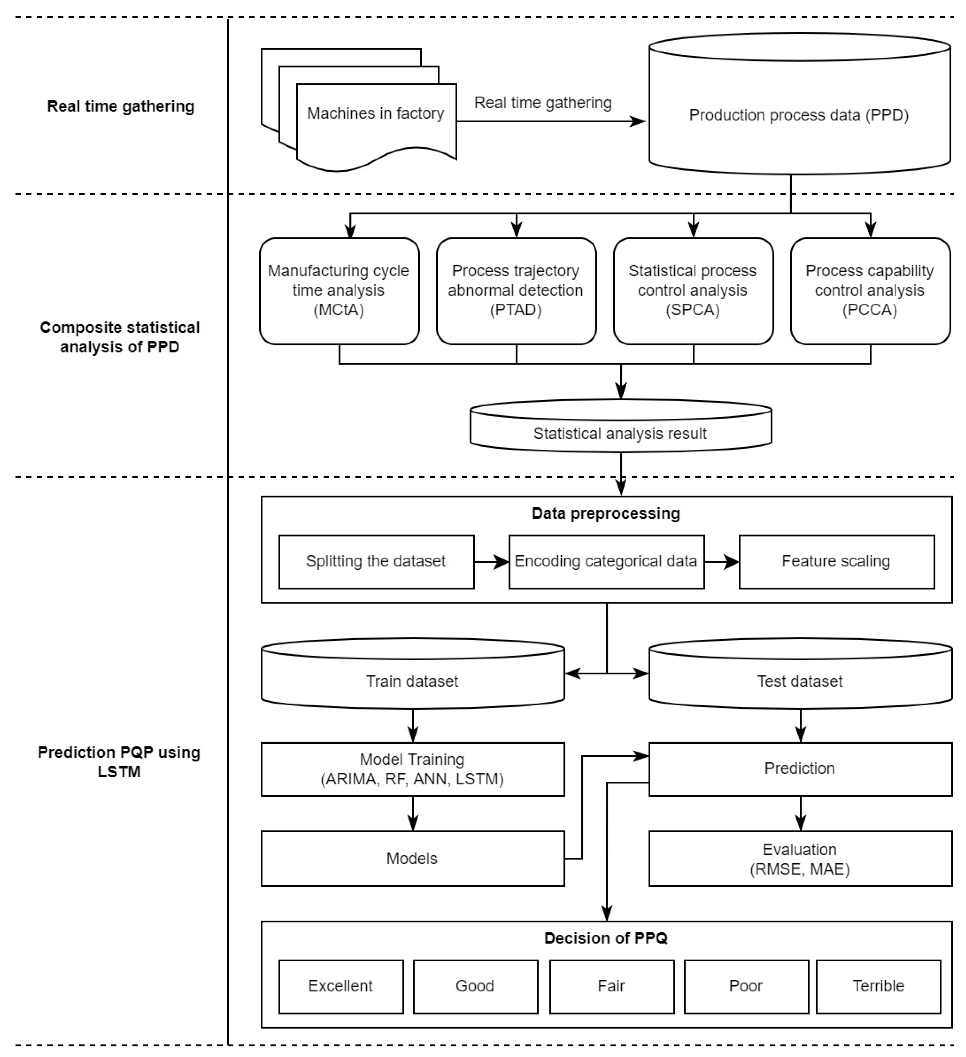
Figure 1 shows the overall flow of the proposed system. The proposed system is divided into three components: real-time data gathering, composite statistical analysis, and prediction of PQP using LSTM.
In
Figure 1, the first step is to perform real-time data collection. Generally, during the manufacturing of products, machines in a factory generate data of different types, such as machine status, production process, and images of testing results. Among them, production process data (PPD) represent the condition values of the machines and the results of the manufactured product. In this paper, we first collect PPD from machines while they are in the production process. Here, to transmit the PPD in real-time to a server system over a wireless or wired network, an Apache Kafka streaming improvement system will be used, as proposed by Leang et al. [
24].
Second, a composite statistical analysis of PPD is proposed to detect abnormal processes in machines, where each machine is manufacturing products periodically. To provide better analysis, four main issues are introduced, including manufacturing cycle time analysis (MCtA), process trajectory of abnormal detection (PTAD), statistical process control analysis (SPCA), and process capability control analysis (PCCA). Here, MCtA is defined as the time it takes to make a product; PTAD identifies abnormal processes when machines are in production. In SPCA [
25], the main parts are only the control charts of type X and R, used to control the quality of processes. Lastly, Cpk of PCCA is applied [
12] to measure the quality of processes and to measure how well the processes are running. The details of this phase will be described in
Section 3.2.
Third, prediction of PQP using LSTM is performed. For this, we first perform a data processing procedure on the dataset obtained from previous composite statistical analysis of the PPD step. Specifically, we perform data splitting, feature scaling, and categorical data encoding procedures. Further, the extracted features are used for training LSTM. Lastly, the Softmax activation function is selected to work with the last layer in the prediction model to classify and output PQP results from 0.00 to 1.00. Here, higher results indicate superior process quality, which might have zero or fewer defective products output. The details of this phase will be provided in
Section 3.3.
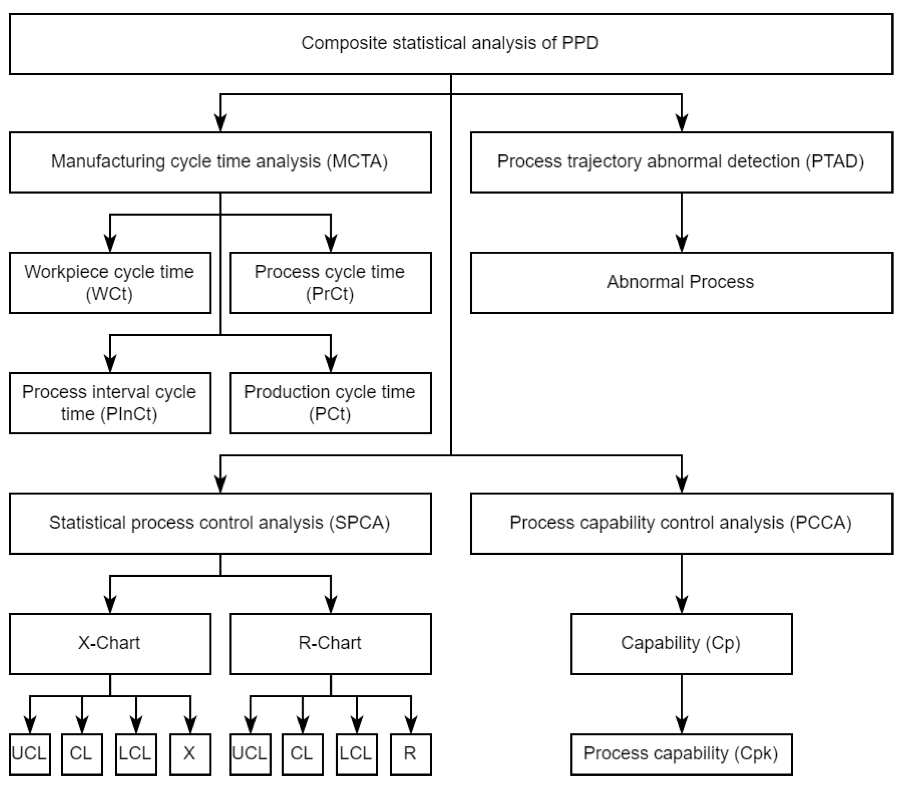
3.2. Composite Statistical Analysis of PPD
In this section, the stage of composite statistical analysis is described with PPD to analyze the quality of production processes. Recall from
Section 2 that, unlike existing studies considering factors that do not fully reflect the manufacturing process of products or consider them separately, we define a PQP as a new process capability and performance measurement tool by simultaneously considering the composite statistical process factors containing MCtA, PTAD, SPCA, and PCCA.
Figure 2 shows the composite statistical analysis of PPD and components of each measurement. The subsequent sections discuss each statistical measurement in detail.
3.2.1. Manufacturing Cycle Time Analysis
Cycle time (Ct) is widely known as an essential measure of performance in the manufacturing industry [
26]. Manufacturing cycle time (MCt) measures the duration of every process move in a production line [
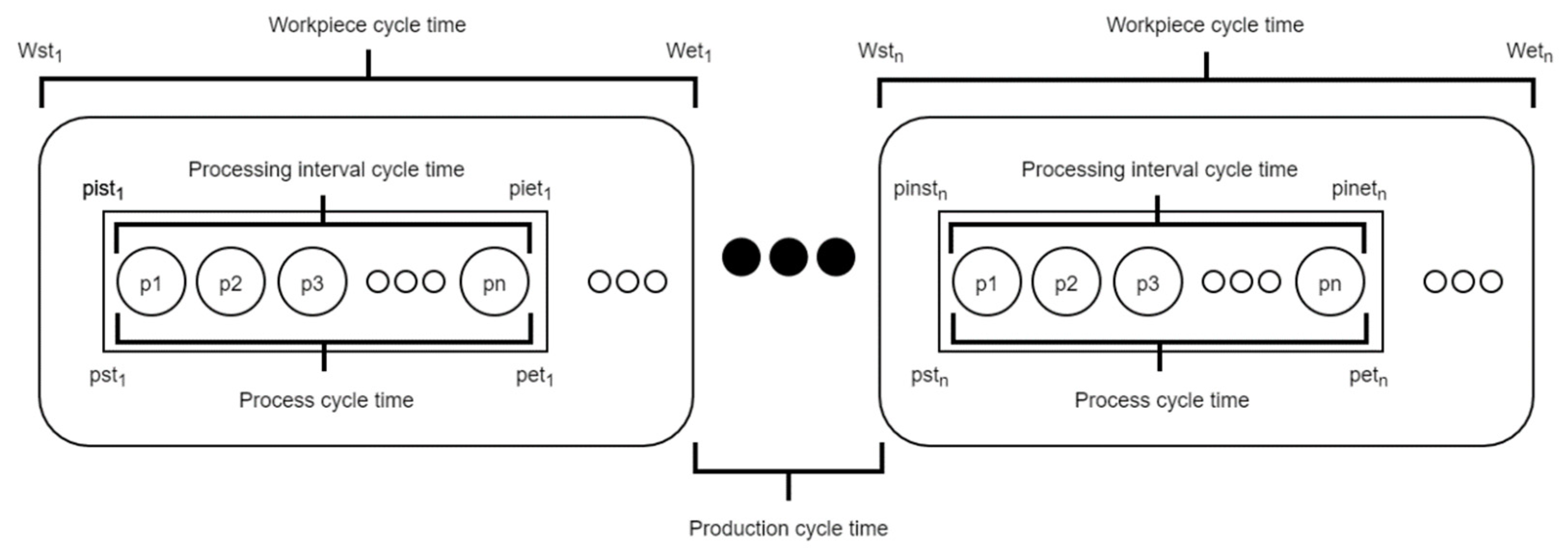
27]. Ct plays an essential role in controlling parameters in the manufacturing process. Specifically, as the manufacturing process may become complex, Ct makes it possible to improve the system by breaking the product cycle times into workpieces to understand the duration of each piece. In other words, operational workpieces can improve product cycle time and increase understanding of the duration of producing each product. In this paper, we propose an MCtA method to analyze duration patterns in producing good and defective products. The proposed MCtA contains four elements: workpiece cycle time (WCt), process cycle time (PrCt), process interval cycle time (PInCt), and production cycle time (PCt).
Figure 3 demonstrates the MCtA proposed in this paper.
From
Figure 3, we can observe that typical manufacturing process contains several
, which is the duration of loading product components into machines. This loading process might start before or after the previous
end time. The calculation of
is given as in the following Equation (1):
where
is the workpiece cycle time of the
ith product and
is the total number of products in the manufacturing process. Besides,
and
are the start time and end time of the
for the
ith product, respectively.
is the duration for producing a single product that may contain many pieces. The calculation of
is shown as in the formula Equation (2):
where
is the process cycle time of the
ith product and
is the total number of products.
and
are the start time and end time of the
for the
ith product, respectively.
In a typical manufacturing process, a product contains many pieces.
refers to the duration of producing a piece of product. For an example, when an imbalanced pressure is in the process of producing a piece of product, this can cause product failure. A high-pressure value has a long duration, calculated by the following Equation (3):
where
is the process interval cycle time of the
ith product and
n is the total number of products.
and
are the start time and end time of the
for the
ith product, respectively.
is the duration from the end of a process of one
in a machine to the start of another
in the same machine. The
is calculated by:
where
is the production cycle time of the
ith product and
is the total number of products;
and
are the start time of the production cycle for the (
i + 1)th and
ith products, respectively.
The aforementioned elements (i.e., , , , and ) enable us to analyze the time it takes to perform one repetition of any product, generally measured from the starting point of one product in a machine to the starting point of another product in the same machine.
3.2.2. Process Trajectory of Abnormal Detection
Recall from
Section 1 that a machine that produces repetitive and periodic products has process condition variables.
Figure 4 shows the values of the process condition variables collected from the machine at times
to
to produce one product. The polyline created connecting these values is defined as a process trajectory. In particular, as the same product is produced periodically, the process trajectory should have almost similar characteristics. Here, we call the trajectory for a good quality product the process of normal trajectory. In
Figure 4, the trajectory of the thick solid line is the process of normal trajectory. Obviously, the process trajectory when defective products are produced will be different from the process of normal trajectory. Finding the problematic trajectory is called the process trajectory of abnormal detection (TAD). TAD has been proposed as a similar concept, which is a useful analysis method in different scenarios, such as abnormal trajectories, abnormal sub trajectories, abnormal road segments, abnormal events, and abnormal moving objects for time series data [
28].
Assume that a process of normal trajectory is given as solid line in
Figure 4 during repeated time period,
and
. Clearly, one product will be repeatedly produced during
seconds. Three process trajectories for three products are considered to calculate the process trajectory of abnormal detection (PTAD) analysis results, which enables us to understand the moving behaviors of production process conditions in machines. Many studies have proposed TAD techniques involving directions, distance-based approaches, historical similarity-based approaches, and density-based and classification-based approaches [
29,
30,
31,
32]. In this paper, we applied the Gaussian normal distribution method for our PPD to detect abnormal trajectories in manufacturing process as shown in Equation (5).
where
is the continuous random variable at a time t,
e is the exponent,
µt is the mean of the random variable
for normal products, and
σt is the standard deviation of random variable
for normal products. The parameters
µt and
σt signify the centering and spread of the Gaussian curve. From
Figure 4, it can also be observed that the density is higher around the mean and decreases rapidly as the distance from the mean increases. This model point distributes around the mean value and spreads to the variance; therefore, it takes two values, mean and variance, to define a Gaussian. In order to know whether a process trajectory is an anomaly, lower and upper threshold values (LT and UT, respectively) are needed. Thus, if the probability of the new data under Gaussian is either higher than UT or lower than LT, it is probably an abnormal process, as it is outside the threshold. In this paper, UT and LT are given as values of Gaussian function with
x = 1.5 × USL and
x = 0.5 × LSL, respectively, where USL is the upper specification limits and LSL is the lower specification limits.
3.2.3. Statistical Process Control Analysis
SPCA is a well-known statistical technique to measure and control the process quality in a manufacturing production line [
13,
14]. It is extensively used in the manufacturing industry to maintain processes while machines are making products. A control chart is one of the essential tools in SPCA, which is used to control and monitor the quality of production processes [
15]. The control chart provides quality characteristics by plotting sample statistics, such as sample process mean or process variance. It can detect early on when a process is out of control, so the manufacturer can correct the system by checking the process or machine conditions. With this, the final products will have fewer defects, and quality will increase.
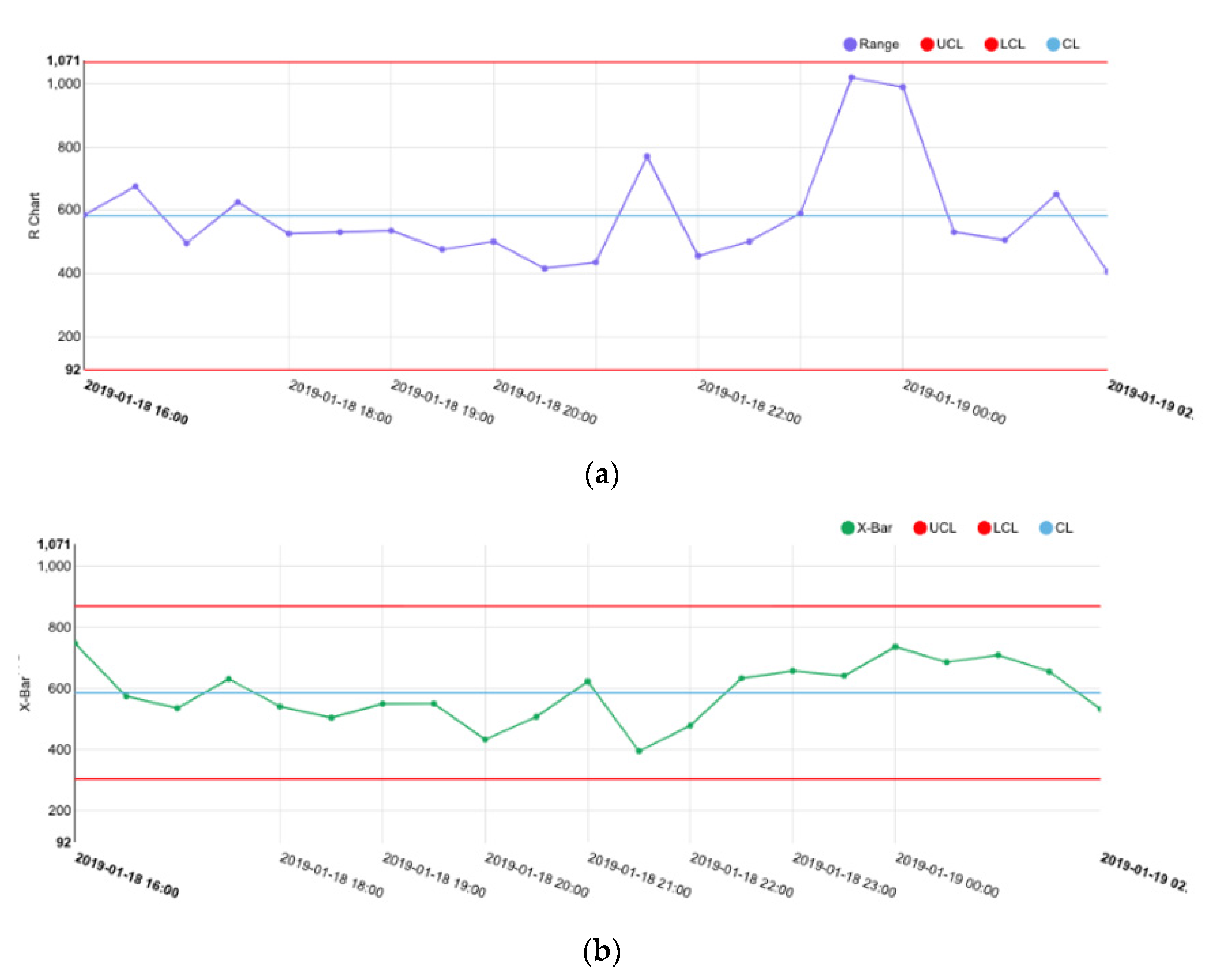
In this paper, X and R control charts are used to monitor processes. Both charts are commonly used in SPCA. They are used separately to measure production process quality. To control the process quality, three straight lines need to be calculated: upper control limit (UCL), centerline (CL), and lower control limit (LCL). The X chart represents the mean value of a process or range value if the process is centered on the target. The R chart represents the standard deviation of the production process if the process spread remains within the right range. The X chart is calculated by the following formulas [
13,
14,
15]:
where
A2 is a coefficient whose value depends on the sample size,
is an average value of the ranges of all observed samples and
is the number of the production process unit per one day. If a process falls outside the control limits there is a statistical certainty that an abnormal process has happened, which is a sign of a defective product.
The R chart uses the sample production process ranges to monitor changes in the spread of a production process. Values are calculated by the following formulas [
13,
14,
15]:
where
and
are coefficients whose values depend on samples of production process size;
is an average value of the ranges of all observed samples and
is the number of the production process unit per one day. If the LCL value of the R and X charts is 0, it is not visible; it is flush with the horizontal axis.
3.2.4. Process Capability Control Analysis
Process capability control (PCC) is well known and widely used as the criteria of choice to measure manufacturing process performance. PCC has achieved acceptable levels of results of significantly lower costs and higher productivity [
9,
10]. PCCA is used to analyze production process quality, which enables manufacturers to understand process quality in real-time [
9,
10]. Furthermore, the capability (Cp) and Cpk formulates the results of PCCA, and are mostly used in manufacturing industries to improve production quality with product design specification limits. Specification limits are set by manufacturers to observe the behavior of production processes, as well as the capability of machines. These limits demonstrate how capable the production process is of producing products and can determine whether a process is working within the specification requirements.
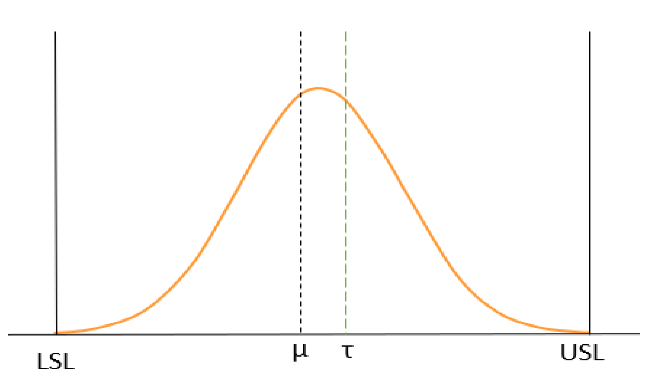
Figure 5 shows the results of PCCA, determined by the LSL and USL.
The specification limits are designed by manufacturers for each machine depending on its capability. The average
µ is the median of the process condition;
τ is the number of the target products of one day. Cp is calculated using the specification limits and the standard deviation, whereas Cpk is calculated using the specification limits, the standard deviation, and the process mean. They are calculated by the following formulas [
8]:
Equation (13) shows the formulas to calculate Cp. Here,
is the standard deviation of the process condition values. If the average values of the process are within the specification limits, the calculated results can measure whether a process is feasible.
Table 1 shows the criteria of process capability.
Equation (14) is a formula to calculate Cpk. Here, k is calculated using Equation (15), and it represents the relationship between Cp and Cpk.
where
is the number of target products of a machine. The calculated result of Cpk is used to determine whether the process is feasible when the average values of the process depart from the median of the specification limits. CpK considers when the average of the processes might not be between the specification limits.
Table 2 shows the criteria of Cpk.
As shown in
Table 1 and
Table 2, if the calculated results of Cp and Cpk are less than 1, the process is unfeasible and does not meet the design specification. Conversely, if the calculated results are greater than or equal 1, the process is feasible and meets the specifications. Cpk can never be greater than Cp. It is possible to have equal values when the actual process average falls in the middle of the design specifications.
3.3. Prediction of PQP Using LSTM
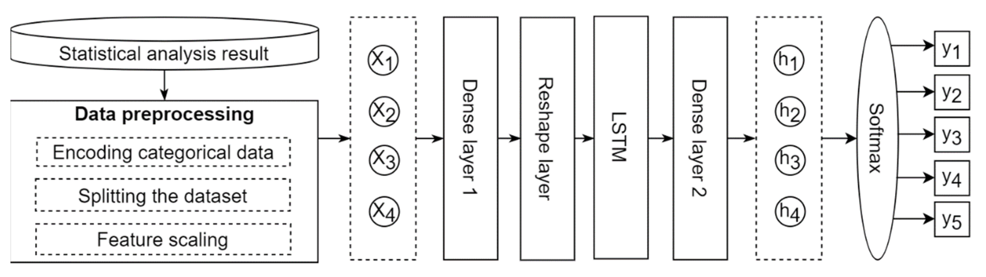
In this section, the prediction stage of PQP is described with composite statistical analysis results for PPD by applying long-term short memory (LSTM) after preprocessing of the analysis data. As shown in
Figure 6, after preprocessing four composite statistical analysis outcomes, MCtA, PTAD, SPCA, and PCCA, a training process using LSTM is described. Here, the preprocessing results will be used as inputs of the dense layer; the outputs of the dense layer will be passed through the reshape layer, the LSTM cells, the dense layer, and finally the Softmax layer to determine the PQP. Details will be provided in subsequent sections.
3.3.1. Process Capability Control Analysis
PPD can be categorized as lower and upper specification limits for a machine as well as the amount, condition values, and start generation and end times for a product made from the machine. PPD is converted into data shown in
Table 3 using the composite statistical analysis methods mentioned from
Section 3.2.
Before applying LSTM to predict PQP, the outcomes of composite statistical analysis in
Table 3 will be preprocessed, as follows:
Encoding categorical data: the label encoder and one hot encoder are used to convert categorical data to numerical data. The categorical data are variables that contain label values rather than numeric values. Many machine learning and deep learning algorithms require all input and output variables to be numeric; therefore, the categorical data must be converted to numerical values.
Splitting dataset: dataset is divided into three subsets: training, validation, and testing sets. The training set is the actual data used to train the model, that is, to fit the parameters. The validation set is the dataset used to tune the hyper-parameter and evaluate a given model fit on the training dataset. The testing set is the dataset used when a model is completely trained, to evaluate how a final model fits the training set.
Feature scaling: This step is also known as data normalization and is used to normalize the range of independent variables or features of data. Feature standardization is used to scale values by applying Z-score normalization. This method is widely used for normalization in machine learning and deep learning models. It calculates the distribution mean and standard deviation for each feature. Then, it subtracts the mean from each feature. After that, it divides each value of each feature by its standard deviation.
3.3.2. Long Short-Term Memory
LSTM is a powerful type of artificial recurrent neural network (RNN) [
33] designed to recognize patterns in sequence data. RNNs can remember input data, which enables this model to predict the next sequence. However, RNNs are only capable of dealing with short-term dependencies [
34], whereas LSTM is capable of learning long-term dependencies. An LSTM is composed of a cell, input gate, output gate, and forget gate. The cell handles remembering values over arbitrary time intervals. The input gate determines whether or not to let new input in and the forget gate determines whether or not to delete information because it is not important or to let that information impact the output at the current time step in the output gate. The LSTM gates are analog, which enables them to do back propagation in the form of a sigmoid; their values range from 0 to 1. This architecture is designed to overcome the limitations of RNN by improving the ability to remember and forget historical data with a long-term period.
The cell gates in LSTM work on the signals they receive. They are similar to the nodes of a neural network. They can block or pass information. They have their own sets of weight, which they can use to filter, and their weight is the modulating input and hidden states, which are adjusted by the learning process of the recurrent network. The LSTM cells learn when open information should enter, leave, or be deleted by adjusting weights of gradient descent and back propagation error. The LSTM can remove or add information to the cell state using structures called gates. The gates are composed of a sigmoid function and a pointwise multiplication operation. The sigmoid function outputs a result from 0 to 1. Let
σ be a sigmoid activation function. To calculate the gate activations, a logistic sigmoid function of the input and weights will be used. The weights are distributed by the LSTM unit via each sequence. The cell and hidden states are under the control of the input and output gates. The states of block input, input, output, cell, hidden, and forget of each sequence are denoted by
z,
i,
o,
c,
h, and
f. A set of weights is denoted as W, and connects between the input and each state in the LSTM unit. The output state manages the information propagated in the previous time step. A new LSTM architecture is introduced in [
35] with forget gates. A forget gate is able to restart the LSTM memory cell after it finishes learning one sequence and before starting a new sequence. The LSTM unit equations can be represented by the following [
36]:
where
is the current input time step.
is the sigmoid function;
denotes the pointwise operation,
is the input weight,
is the recurrent weight, and
is the bias. To predict the next sequence of the production process quality, the statistical process analysis results are the most important features; they are used to train and predict future process quality in the LSTM model.
3.3.3. Softmax Classification
Generally, the Softmax function is used in the final layer of the deep learning prediction model including LSTM to classify predicted results of a final output layer. The Softmax function takes as input a vector of
h real numbers and normalizes it into a probability distribution consisting of
h probabilities. Here
h is the number of predicted classes. Even if some vector components could be negative, or greater than one, and might not sum to 1, after applying the Softmax function, each component will be in the interval (0.0, 1.0) and the sum of the components will be 1, so it can be interpreted as a probability. We use the Softmax function to output the PQP result with the following formula:
We used this algorithm to classify the predicted result of the LSTM output layer, where PQP
i is the Softmax output for the
ith value in the input vector of size
N. The input vectors are [
a1,
a2,
a3,
…,
aN], and PQP
i is always positive. The standard exponential function is applied to each element PQP
i, and the values are normalized by dividing by the sum of all the exponents. This normalization ensures that the sum of the components of the output vector PQP is 1; PQP
i is greater than 0 because of the exponents. Because the numerator appears in the denominator, summed up with some other positive numbers, PQP
i is smaller than 1. Decision criteria for PQP status were decided with many experiments by checking machine feasibility and operation status conditions according to the PQP value.
Table 4 shows the criteria for production process stability. Softmax classifier results from 0.50 to 1.00 are the best results, which mean the processes might be capable of producing products without any defects. On the other hand, if the results range from 0.00 to 0.50, the quality in the criteria table is poor or terrible, which indicates that the process is so bad that it needs to be improved as soon as possible to prevent defective products.
3.3.4. Evaluation Metrics
Evaluation metrics measure the applicability of a learned model and explain the performance of the model. They allow us to make improvements and continue until the learned model achieves a desirable accuracy. There are different kinds of evaluation metrics for the predictive accuracy of the model. Selecting evaluation metrics completely depends on the type of model and the implementation plan. In this work, a confusion matrix is used to evaluate our prediction model. The confusion matrix is an elevation metric used to measure the performance of a classification model. In predictive analytics, a confusion matrix is used, as shown in
Table 5, and it has two rows and two columns that show the numbers of false positives, false negatives, true positives, and true negatives. Each row of the matrix in the confusion matrix table represents a predicted class, while each column represents an actual class.
The confusion matrix can be used to measure the performance of the classification model in different approaches, as shown in
Table 6. This table shows the calculation of certain error metrics of the confusion matrix, such as accuracy, sensitivity (true positive rate), specificity (false positive rate), recall, and precision. The sensitivity corresponds to the proportion of the positive class that predicted correctly, while the specificity corresponds to the proportion of the negative class that is mistakenly considered to be positive; both have values in the range from 0 to 1.
4. Results
The implementation of this system is based on a web-based application using the Java Spring Framework. The results are presented using different kinds of plots, bar charts, tables, and some text to explain the different visualizations. The plots and bar charts are developed using D3.js [
37], a JavaScript library for manipulating documents based on data. The deep learning models, such as LSTM in this system, are developed using Deeplearning4j [
38], which is written in Java, and is a computing framework with wide support for deep learning algorithms. In this paper, to analyze and make predictions, the dataset for PPD is collected from the automotive industry. In this paper, we made a single record of one PPD consisting of a machine name, starting and ending times to make a product, number of products, process condition values during making products, USL and LSL of process conditions. We used pressure values as process conditions. The total size of PPD is 29,365,980 records, collected from a period of 9 months. The data are divided into three subsets: training set 50%, validation 25%, and testing set 25%.
4.1. System Architecture
The implementation architecture of the proposed method can be described in the interaction of two different parts, the system environment layer and the web application, as shown in
Figure 7. System environment layer is designed to collect PPD based on Hadoop environment [
39,
40]. Using Apache Kafka, this part is responsible for gathering data from manufacturing; gathered data is stored into Apache HBase. The second part is the web application part, which communicates with the first part to retrieve data. If the specific row key index of HBase is known, the HBase client can be used to retrieve data from HBase. Otherwise, instead of retrieving data from HBase, the phoenix client is used with the secondary index. The Hadoop cluster is installed using five servers.
Table 7 shows the server specifications, such as RAM, OS, CPU, and HDD. After setting up a Hadoop cluster, we install the other four main projects of Apache Kafka, Apache zookeeper, Apache HBase, and Apache phoenix in the Hadoop cluster [
41,
42,
43].
4.2. Result of Composite Statistical Analysis Using PPD
In the proposed system, the user enters a start date and an end date to analyze PPD, and collects all PPD within the period. With the data, we describe the composite statistical process analysis, such as SPC type X and R charts with PCCA result, WCt analysis, and PTAD in this section.
Figure 8 shows the results of the X and R charts for a certain period of time in the real-world manufacturing process. The centerline is the average of all production process ranges. The red points indicate processes that fail at least one of the tests and are not in control. If the same point fails multiple tests, the point is labeled with the lowest test number, to avoid cluttering the graph. The out-of-control points can lead the production process to produce many defective products; therefore, if the chart shows out-of-control points, the manufacturers need to investigate those points to solve the problem as soon as possible. As can be observed from the figure, both charts are stable; no points are out of control in the charts.
For one workpiece,
Figure 9 shows the WCt results with the other three sub WCt, such as PrCt, PInCt, and PCt. Cycle time is the duration that it takes to complete a production run divided by the number of acceptable workpieces produced.
Figure 10 shows the process trajectory of abnormal detection with Gaussian distribution. The histogram combines all three processes into one histogram plot. The Gaussian is a distribution that is parameterized by the average and standard deviation. With the Gaussian, we can know whether a piece of data is an anomaly based on a threshold value. If the probability of the data under the Gaussian is higher or lower than the threshold, it is probably an anomaly. We can define the threshold by looking at the plot of the Gaussian, above. Anomaly data would be data that fall under the low probability areas of the Gaussian, because being in the low probability area, that data is highly unlikely to be distributed in the distribution. Those low probability areas are the left and the right tails of the Gaussian.
4.3. Result of Predicting PQP Using LSTM
After the statistical analysis results are preprocessed, they are converted into the shape of LSTM. To use LSTM, in this paper, we create a sequential model with four layers including a input dense layer, reshape layer, LSTM cell layer, and output dense layer. The sequential model can have only one structure. Each layer of the sequential model is stacked by adding it to the top of the stack, while each input of a new layer is interconnected with specific outputs from the previous neural layer.
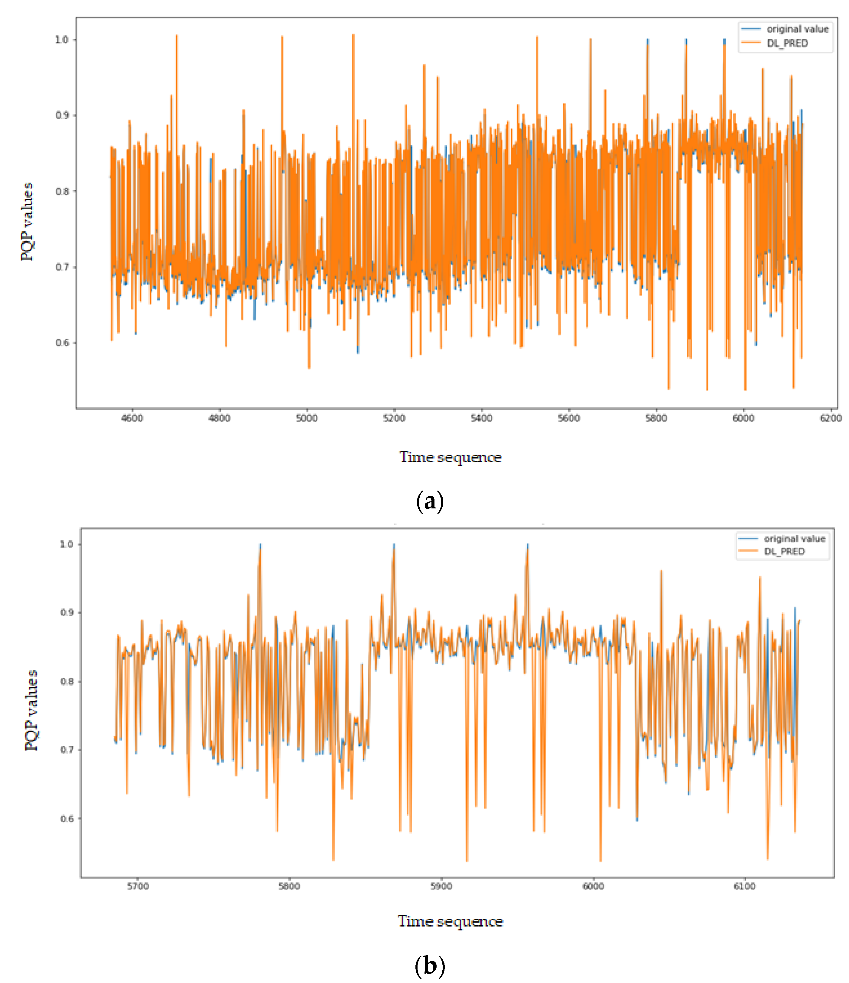
Figure 11a shows the results of prediction for all PQP, while
Figure 11b shows the predicting of PQP for one day. These plots show both original values and LSTM prediction values. The orange line is the prediction results, while the blue line is the actual data.
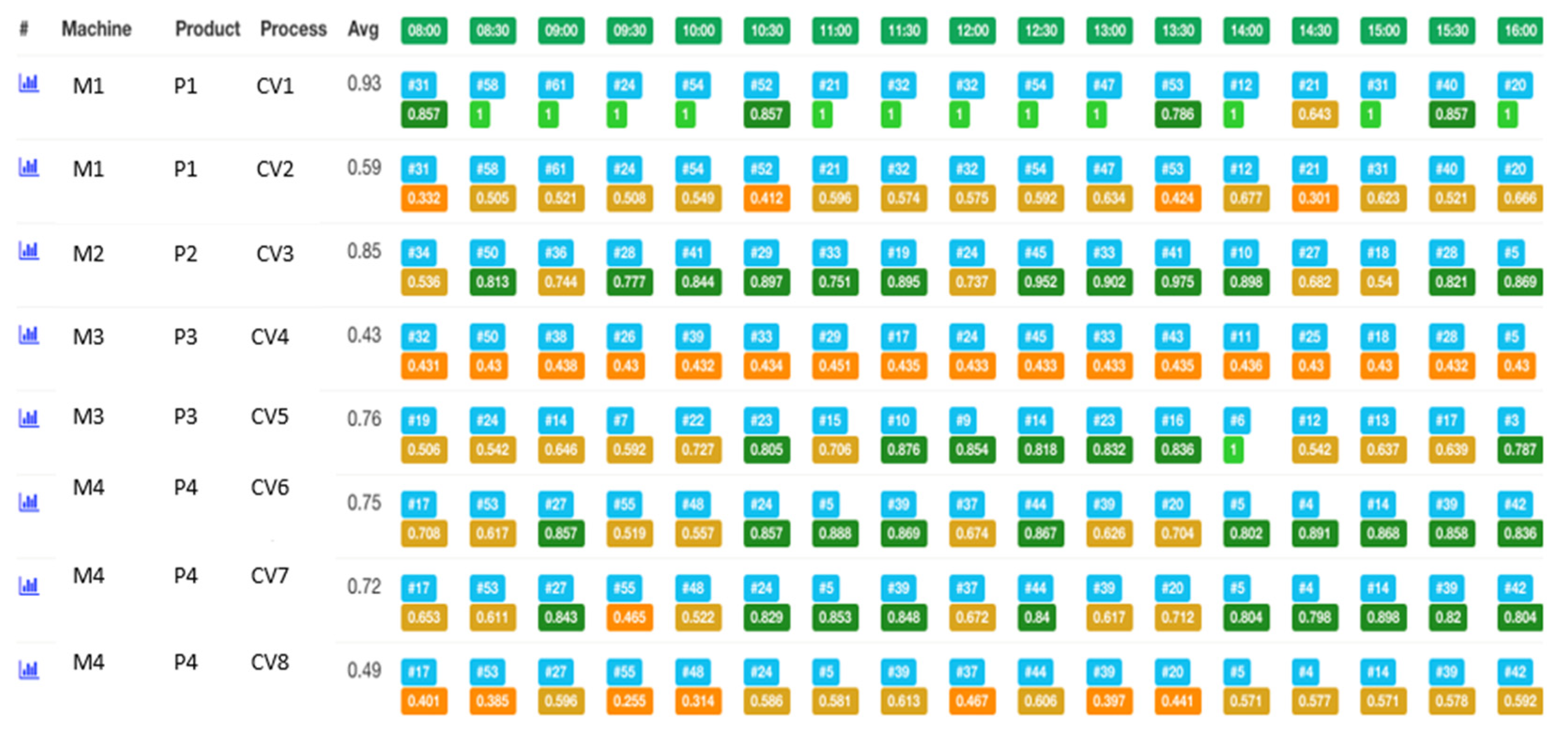
Figure 12 provides a visualization of the prediction and estimation results on the web page by using D3js library. Here, the results range from 0.0 to 1.0; the higher probability is considered to represent stronger process quality, which could produce products without any defects. We also show detailed information in the table to allow manufacturers to see the production process stability and to analyze the prediction results.
4.4. Result of Model Comparison
In order to show the effectiveness of our proposed approach, we compare the LSTM prediction model with the random forest algorithm, ARIMA, and ANN. We set 1000 as the number of epochs, 0.01 as the learning rate, five as the batch size, and Softmax as the activation for the LSTM model. For the random forest model, a 1000 n_estimator, TRUE oob_score, and 42 random_state are given. The 1000 number of epochs, 0.01 learning rate, five batch size, and Softmax activation are set for the ANN model. As mentioned above, we use 29,365,980 PPD records, which consist of 50% training set, 25% validation set, and 25% testing set. First, we split the dataset into training, test, and validation data. Furthermore, the training data is divided into subsets that use the different folds as validation data. We also nominate several values for each hyperparameter of each model. Then, we find the best parameters using training subsets and hyperparameter options grid search. For testing, we utilized the grid search method.
Detailed testing results of the models are presented in
Table 8. As shown in this table, among the three models, the LSTM model achieved the highest accuracy. The random forest achieves a performance closest to that of our proposed approach, but its ability to estimate and predict algorithms is still considerably lower than that of the proposed method.
We applied the methods proposed above to perform a five-step prediction of PQP for a specific facility every 30 min. Therefore, since this problem is fundamentally a classification problem, it can be observed that the performance of the random forest method, which is used as a representative classification method in machine learning, is relatively higher than that of the ARIMA method, which is used as a prediction method according to time. If big data used for the experiment in this paper is used, the accuracy of the deep learning method will be higher than that of the machine learning method. Therefore, the LSTM method is widely used to know the classification results over time in deep learning techniques. As the PQP prediction problem presented in this paper is of the same type, it can be observed that the experimental results using LSTM are relatively high compared to the ANN technique applied as a deep learning technique.
5. Conclusions
In this paper, we have proposed a method for predicting PQP using statistical analysis and long short-term memory. There are several findings of this study. First, no studies sufficiently consider stability and normality of process conditional variables and time-series work patterns, which we define as work repeatability. And we also have proposed a method for estimating process capability and performance by comprehensively considering periodic and repetitive work pattern characteristics over time. Second, statistical, machine learning, and deep learning analysis can be applied to predict PQP characteristics and estimate the anomalies in the production process. To do it better, we have demonstrated that LSTM, a deep learning algorithm-based method, can evaluate the stability of the production process with the highest accuracy compared with other state-of-the-art ANN, RF, and ANN methods. One of the essential applications of predicting PQP characteristics is predictive maintenance in smart manufacturing. That is, we can collect process condition variables over time by monitoring the states of product manufacturing and use these variables to predict possible failures, process capability, and performance in the future. Third, the result of this study is exemplified by a real case study, a smart manufacturing system in the automotive industry, to verify the product quality improvement. The approach proposed in this research is currently used by quality management departments in the manufacturing industry to monitor the production process and prevent product defects. From the results demonstrated in this study, we can conclude that utilizing statistical analysis involving MCtA, PCCA, PTAD, and SPCA can effectively determine PQP in manufacturing processes. In addition, the application of deep learning methods is found to be effective in predicting PQP in future processes and determining the optimal working condition, which can be helpful for manufacturing operators. In other words, our proposed model accomplished its goals, and so is effective and beneficial for the automotive industry, which can identify and prevent quality defects of final products, increasing overall product quality significantly.
During this research, some challenges were found that could potentially be considered as future work. Some limitations with the dataset used for training and validating the prediction model need to be addressed. Future research will collect more valuable data from machines in the manufacturing industry to improve our dataset. We suppose that our proposed approach will perform better after conducting experiments with a larger dataset. Furthermore, we intend to explore more feature extraction from the original dataset by using various types of process analysis to improve the accuracy of the prediction model and other types of unsupervised feature learning. In addition, we plan to improve the prediction algorithm by optimization and by hyper-parameter learning model.
Author Contributions
Conceptualization, T.P. and K.-H.Y.; methodology, T.P.; formal analysis, T.P.; data curation, T.P., S.-H.K. and G.-A.R.; writing—original draft preparation, T.P.; writing—review and editing, T.C. and A.N.; visualization, T.P.; supervision, K.-H.Y. and A.N.; project administration, K.-H.Y.; funding acquisition, K.-H.Y. and A.N. All authors have read and agreed to the published version of the manuscript.
Funding
This work was supported by the Technology Innovation Program (2004367, development of a cloud big data platform for innovative manufacturing in the ceramic industry) funded by the Ministry of Trade, Industry & Energy (MOTIE, Korea), and by the MSIT (Ministry of Science and ICT), Korea, under the Grand Information Technology Research Center support program (IITP-2021-2020-0-01462) supervised by the IITP (Institute for Information & Communications Technology Planning & Evaluation).
Conflicts of Interest
The authors declare that there are no conflicts of interest regarding the publication of this paper.
References
- Windmann, S.; Maier, A.; Niggemann, O.; Frey, C.; Bernardi, A.; Gu, Y.; Pfrommer, H.; Steckel, T.; Kruger, M.; Kraus, R. Big Data Analysis of Manufacturing Processes. J. Phys. Conf. Ser. 2015, 659, 012055. [Google Scholar] [CrossRef]
- Gerbert, P.; Lorenz, M.; Rubmann, M.; Waldner, M.; Justus, J.; Engel, P.; Harnisch, M. Industry 4.0: The Future of Productivity and Growth in Manufacturing Industries. Available online: https://www.bcg.com/publications/2015/engineered_products_project_business_industry_4_future_productivity_growth_manufacturing_industries.aspx (accessed on 10 January 2022).
- Zaslavsky, A.; Perera, C.; Georgakopoulous, D. Sensing as a Service and Big Data. In Proceedings of the International Conference on Advances in Cloud Computing (ACC), Bangalore, India, 22 July 2012; pp. 21–29. [Google Scholar]
- Koh, G.; Yu, H.; Kim, S. Secret Key and Tag Generation for IIoT Systems Based on Edge Computing. J. Multimed. Inf. Syst. 2021, 8, 57–60. [Google Scholar] [CrossRef]
- Jenny, H.; Maria, S.; Kusiak, A. Data Mining in Manufacturing: A Review. J. Manuf. Sci. Eng. 2006, 128, 969–976. [Google Scholar]
- Changchao, G.; Yihai, H.; Xiao, H.; Zhaoxiang, C. Product quality oriented predictive maintenance strategy for manufacturing systems. In Proceedings of the Prognostics and System Health Management Conference, Harbin, China, 9–12 July 2017. [Google Scholar]
- Lee, K.M.; Yoo, J.; Kim, S.-W.; Lee, J.-H.; Hong, J. Autonomic machine learning platform. Int. J. Inf. Manag. 2019, 49, 491–501. [Google Scholar] [CrossRef]
- Rodrig, R.N. Recent Developments in Process Capability Analysis. J. Qual. Technol. 2018, 24, 176–187. [Google Scholar] [CrossRef]
- Spiring, F.; Leung, B.; Cheng, S.W.; Yeung, A. A Bibliography of Process Capability Papers. Qual. Reliab. Eng. Int. 2003, 445–460. [Google Scholar] [CrossRef]
- Spiring, F.A. A Unifying Approach to Process Capability Indices. J. Qual. Technol. 2018, 29, 49–58. [Google Scholar] [CrossRef]
- Wu, C.W.; Pearn, W.L.; Kotz, S. An overview of theory and practice on process capability indices for quality assurance. Int. J. Prod. Econ. 2019, 117, 338–359. [Google Scholar] [CrossRef]
- Mottonen, M.; Belt, P.; Harkonen, J.; Haapasalo, H.; Kess, P. Manufacturing Process Capability and Specification Limits. Open Ind. Manuf. Eng. J. 2008, 1, 29–36. [Google Scholar] [CrossRef]
- Montgomery, D.C. Introduction to Statistical Quality Control, 6th ed.; John Wiley & Sons: Hoboken, NJ, USA, 2009. [Google Scholar]
- Zheng, Y.; Geng, Q.; He, R. The Application of Control Chart Based on Bayesian Statistic in Equipment Maintenance Quality Control. In Proceedings of the International Conference on Quality, Reliability, Risk, Maintenance, and Safety Engineering, Chengdu, China, 15–18 July 2013; pp. 1654–1657. [Google Scholar]
- Zhang, N.F. A Statistical Control Chart for Stationary Process Data. J. Tech. 2012, 40, 24–38. [Google Scholar] [CrossRef]
- Peng, S.; Zhou, M. Production cycle-time analysis based on sensor-based stage Petri nets for automated manufacturing systems. In Proceedings of the IEEE International Conference on Robotics and Automation, Taipei, Taiwan, 14–19 September 2003; Volume 3, pp. 4300–4305. [Google Scholar]
- Diallo, M.S.; Mokeddem, S.A.; Braud, A.; Frey, G.; Lachiche, N. Identifying Benchmarks for Failure Prediction in Industry 4.0. Informatics 2021, 8, 68. [Google Scholar] [CrossRef]
- Wolfram, W.; Christina, F.; Thomas, L. Early Detection of Critical Faults Using Time-Series Analysis on Heterogenous Information Systems in the Automotive Industry. In Proceedings of the Third International Conference on Data Analytics, Rome, Italy, 24–28 August 2014; pp. 70–75. [Google Scholar]
- Ahmad, S.; Lavin, A.; Purdy, S.; Agha, Z. Unsupervised rea-time anomaly detection for streaming data. Neurocomputing 2017, 262, 134–147. [Google Scholar] [CrossRef]
- Filonov, P.; Lavrentyev, A.; Vorontsov, A. Multivariate Industrial Time Series with Cyber Attack Simulation: Fault Detection Using an LSTM-based Predictive Data Model. In Proceedings of the NIPS Time Series Workshop, Barcelona, Spain, 26 December 2016. [Google Scholar]
- Borith, T.; Bakhit, S.; Nasridinov, A.; Yoo, K.-H. Prediction of Machine Inactivation Status Using Statistical Feature Extraction and Machine Learning. Appl. Sci. 2020, 10, 7413. [Google Scholar] [CrossRef]
- Zhang, W.; Guo, W.; Liu, X.; Liu, Y.; Zhou, J.; Li, B.; Lu, Q.; Yang, S. LSTM-Based Analysis of Industrial IoT Equipment. IEEE Access 2018, 6, 23551–23560. [Google Scholar] [CrossRef]
- Ean, S.; Bazarbaev, M.; Lee, K.M.; Nasridinov, A.; Yoo, K.-H. Dynamic programming-based computation of an optimal tap working pattern in nonferrous arc furnace. J. Supercomput. 2021, 78, 640–666. [Google Scholar] [CrossRef]
- Leang, B.; Ean, S.; Ryu, G.; Yoo, K.H. Improvement of Kafka Streaming Using Partition and Multi-Threading in Big Data Environment. Sensor 2019, 1, 134. [Google Scholar] [CrossRef] [Green Version]
- Vanli, O.A.; Castillo, E.D. Statistical Process Control in Manufacturing. Encyclopedia of Systems and Control; Springer: London, UK, 2014. [Google Scholar]
- Leachman, R.C.; Ding, S. Excursion Yield Loss and Cycle Time Reduction in Semiconductor Manufacturing. IEEE Trans. Autom. Sci. Eng. 2010, 8, 112–117. [Google Scholar] [CrossRef]
- Rodrigues, L.L.R.; Patel, R.; Gopalakrishna, B.; Shetty, P.K.; Rao, B.R.S. Affect of Production cycle time in manufacturing supply chain management: A system dynamics approach. In Proceedings of the IEEE International Conference on Management of Innovation & Technology, Singapore, 2–5 June 2010; pp. 146–150. [Google Scholar]
- Lee, J.G.; Han, J.; Li, X. Trajectory Outlier Detection: A Partition-and-Detection Framework. In Proceedings of the International Conference on Data Engineering, Cancun, Mexico, 7–12 April 2008; pp. 140–149. [Google Scholar]
- Liu, Z.; Pi, D.; Jiang, J. Density-based trajectory outlier detection algorithm. J. Syst. Eng. Electron. 2013, 24, 335–340. [Google Scholar] [CrossRef]
- Ma, X.M.; Ngan, H.Y.T.; Liu, W. Density-based Outlier Detection by Local Outlier Factor on Large-scale Traffic Data. Electron. Imaging 2016, 14, 1–4. [Google Scholar]
- Ying, X.; Xu, Z.; Yin, W.G. Cluster-based Congestion Outlier Detection Method on Trajectory Data. In Proceedings of the Sixth International Conference on Fuzzy System and Knowledge Discovery, Tianjin, China, 14–16 August 2009. [Google Scholar]
- Wu, H.; Sun, W.; Zheng, B. A Fast Trajectory Outlier Detection Approach via Driving Behavior Modeling. In Proceedings of the ACM on Conference on Information and Knowledge Management, Singapore, 6–10 November 2017; pp. 837–846. [Google Scholar]
- Hochreiter, S.; Schmidhuber, J. Long Short-term Memory. Neural Comput. 1997, 9, 1735–1780. [Google Scholar] [CrossRef]
- Gers, F.A.; Schraudolph, N.N.; Schmidhuber, J. Learning Precise Timing with LSTM Recurrent Networks. J. Mach. Learn. Res. 2002, 3, 115–143. [Google Scholar]
- Gers, F.A.; Schmidhuber, J.; Cummins, F.A. Learning to Forget: Continual Prediction with LSTM. Neural Comput. 2002, 12, 2451–2471. [Google Scholar] [CrossRef] [PubMed]
- Greff, K.; Srivastava, R.K.; Koutnik, J.; Steunebrink, B.R.; Schmidhuber, J. LSTM: A Search Space Odyssey. IEEE Trans. Neural Netw. Learn. Syst. 2017, 28, 2222–2232. [Google Scholar] [CrossRef] [PubMed] [Green Version]
- D3.js—Data-Driven Documents. Available online: https://d3js.org (accessed on 29 November 2021).
- Deeplearning4j. Available online: https://deeplearning4j.konduit.ai (accessed on 29 November 2021).
- Harezlak, K.; Skowron, R. Performance Aspects of Migrating a Web Application from a Relational to a NoSQL Database. In Proceedings of the Beyond Databases, Architectures and Structures, Ustron, Poland, 26–29 July 2015; Volume 521, pp. 107–115. [Google Scholar]
- Zhao, G.; Li, L.; Li, Z.; Lin, Q. Multiple Nested Schema of HBase for Migration from SQL. In Proceedings of the 2014 Ninth International Conference on P2P, Parallel, Grid, Cloud and Internet Computing, Guangdong, China, 8–10 November 2014; pp. 338–343. [Google Scholar]
- Dean, J.; Ghemawat, S. MapReduce: Simplified Data Processing on Large Clusters. In Proceedings of the Sixth Symposium on Operating System Design and Implementation, San Francisco, CA, USA, 6–8 December 2004; Volume 6, pp. 137–150. [Google Scholar]
- Gupta, K.; Sachdev, A.; Sureka, A. Performance Comparison and Programming Alpha-miner Algorithm in Relational Database Query Language and NoSQL Column-Oriented Using Apache Phoenix. In Proceedings of the Eighth International Conference on Computer Science & Software Engineering, Yokohama, Japan, 13–15 July 2015; pp. 113–118. [Google Scholar]
- Hiraman, B.R.; Chapte, V.M.; Abhijeet, C.K. A Study of Apache Kafka in Big Data Stream Processing. In Proceedings of the International Conference on Information, Communication, Engineering and Technology, Pune, India, 29–31 August 2018; pp. 1–3. [Google Scholar]
Figure 1.
Overall flow of the proposed system.
Figure 1.
Overall flow of the proposed system.
Figure 2.
Composite statistical analysis of PPA.
Figure 2.
Composite statistical analysis of PPA.
Figure 3.
Process of MCtA.
Figure 3.
Process of MCtA.
Figure 4.
Multiple processes (i.e., normal and abnormal) trajectories for one machine.
Figure 4.
Multiple processes (i.e., normal and abnormal) trajectories for one machine.
Figure 5.
Process capability control analysis.
Figure 5.
Process capability control analysis.
Figure 6.
Procedure for applying LSTM to decide PQP.
Figure 6.
Procedure for applying LSTM to decide PQP.
Figure 7.
Implementation architecture of the proposed method.
Figure 7.
Implementation architecture of the proposed method.
Figure 8.
Result of various charts in real-world manufacturing processes; (a) result of X chart and (b) result of R chart.
Figure 8.
Result of various charts in real-world manufacturing processes; (a) result of X chart and (b) result of R chart.
Figure 9.
Results of manufacturing cycle time calculation in real-world manufacturing process; (a) WCt, (b) PInCt, (c) PrCt and (d) PCt.
Figure 9.
Results of manufacturing cycle time calculation in real-world manufacturing process; (a) WCt, (b) PInCt, (c) PrCt and (d) PCt.
Figure 10.
Results of multiple process trajectories of abnormal detection in real-world manufacturing process.
Figure 10.
Results of multiple process trajectories of abnormal detection in real-world manufacturing process.
Figure 11.
Result of prediction PQP using LSTM; (a) result of overall PQP prediction and (b) result of PQP prediction for one day.
Figure 11.
Result of prediction PQP using LSTM; (a) result of overall PQP prediction and (b) result of PQP prediction for one day.
Figure 12.
Web-based GUI for predicting PQP in real-world manufacturing process.
Figure 12.
Web-based GUI for predicting PQP in real-world manufacturing process.
Table 1.
Criteria of process capability, Cp.
Table 1.
Criteria of process capability, Cp.
| Division | Quality | Normal Production Rate | Failure Production Rate |
|---|
| Cp ≥ 1.68 | Excellent | 99.999991% | 0.000009% |
| 1.34 ≤ Cp ≤ 1.67 | Very good | 99.999943% | 0.000057% |
| 1.01 ≤ Cp ≤ 1.33 | Good | 99.9937% | 0.0063% |
| 0.68 ≤ Cp ≤ 1.00 | Fair | 99.73% | 0.27% |
| 0.00 ≤ Cp ≤ 0.67 | Poor | 95.45% | 4.65% |
Table 2.
Criteria of process capability index, Cpk.
Table 2.
Criteria of process capability index, Cpk.
| Division | Quality | Normal Production Rate | Failure Production Rate |
|---|
| Cpk < 0.33 | Terrible | 99.85% | 1.15% |
| 0.33~0.67 | Very poor | 95.45% | 4.65% |
| 0.67~1.00 | Poor | 99.73% | 0.27% |
| 1.00~1.33 | Average | 99.9937% | 0.0063% |
| 1.33~1.67 | Good | 99.999943% | 0.000057% |
| 1.67~2.00 | Very good | 99.999991% | 0.000009% |
| Cpk > 2.00 | Excellent | 99.999998% | 0.000002% |
Table 3.
Outcomes of composite statistical analysis.
Table 3.
Outcomes of composite statistical analysis.
| Classification | Outcomes | Data Type |
|---|
| MCtA | Workpiece cycle time (WCt) | Long |
| Process cycle time (PrCt) | Long |
| Process interval cycle time (PInCt) | Long |
| Production cycle time (PCt) | Long |
| PTAD | Abnormal process status value | Float |
| SPCA | Mean value of a production process condition X | Float |
| Upper control limit of X | Float |
| Lower control limit of X | Float |
| Standard deviation R of X | Float |
| Upper control limit of R | Float |
| Lower control limit of R | Float |
| PCCA | Process capability Cp | Float |
| Process capability index Cpk | Float |
Table 4.
Criteria of PQP.
Table 4.
Criteria of PQP.
| PQP Value | Quality |
|---|
| 1.00 | Excellent |
| 0.75–0.99 | Good |
| 0.50–0.75 | Fair |
| 0.25–0.50 | Poor |
| 0.00–0.25 | Terrible |
Table 5.
Confusion matrix.
Table 5.
Confusion matrix.
| | Predicted Classes |
|---|
| Positive | Negative |
|---|
| Actual Class | Positive | True positive (TP) | False negative (FN) |
| Negative | False positive (FP) | True negative (TN) |
Table 6.
Evaluation metrics.
Table 6.
Evaluation metrics.
| Error Metric | Definition |
|---|
| Accuracy | TP + TN/(TP + TN + FP + FN) |
| Sensitivity | TP/(TP + FN) |
| Specificity | TN/(TN + FP) |
| Precision | TP/(TP + FP) |
| Recall | TP/(TP + FN) |
Table 7.
Server specification for data storage with Hadoop ecosystem.
Table 7.
Server specification for data storage with Hadoop ecosystem.
| Division | Specification |
|---|
| Ram | 64 GB |
| OS | Ubuntu 16.0 |
| CPU | Intel(R) Xeon(R) Silver 4114 CPC @ 2.20 GHz |
| HDD | 2T,2T,1T,1T |
Table 8.
Result of model comparison.
Table 8.
Result of model comparison.
| Model | Recall | Precision | Accuracy |
|---|
| LSTM | 0.91 | 0.73 | 0.93 |
| ANN | 0.90 | 0.70 | 0.83 |
| Random Forest | 0.92 | 0.65 | 0.89 |
| ARIMA | 0.89 | 0.69 | 0.77 |
| Publisher’s Note: MDPI stays neutral with regard to jurisdictional claims in published maps and institutional affiliations. |
© 2022 by the authors. Licensee MDPI, Basel, Switzerland. This article is an open access article distributed under the terms and conditions of the Creative Commons Attribution (CC BY) license (https://creativecommons.org/licenses/by/4.0/).


 ,
, 


