
Modular Robotic Design and Reconfiguring Path Planning


Abstract
:1. Introduction
2. Robotic Design and Modeling
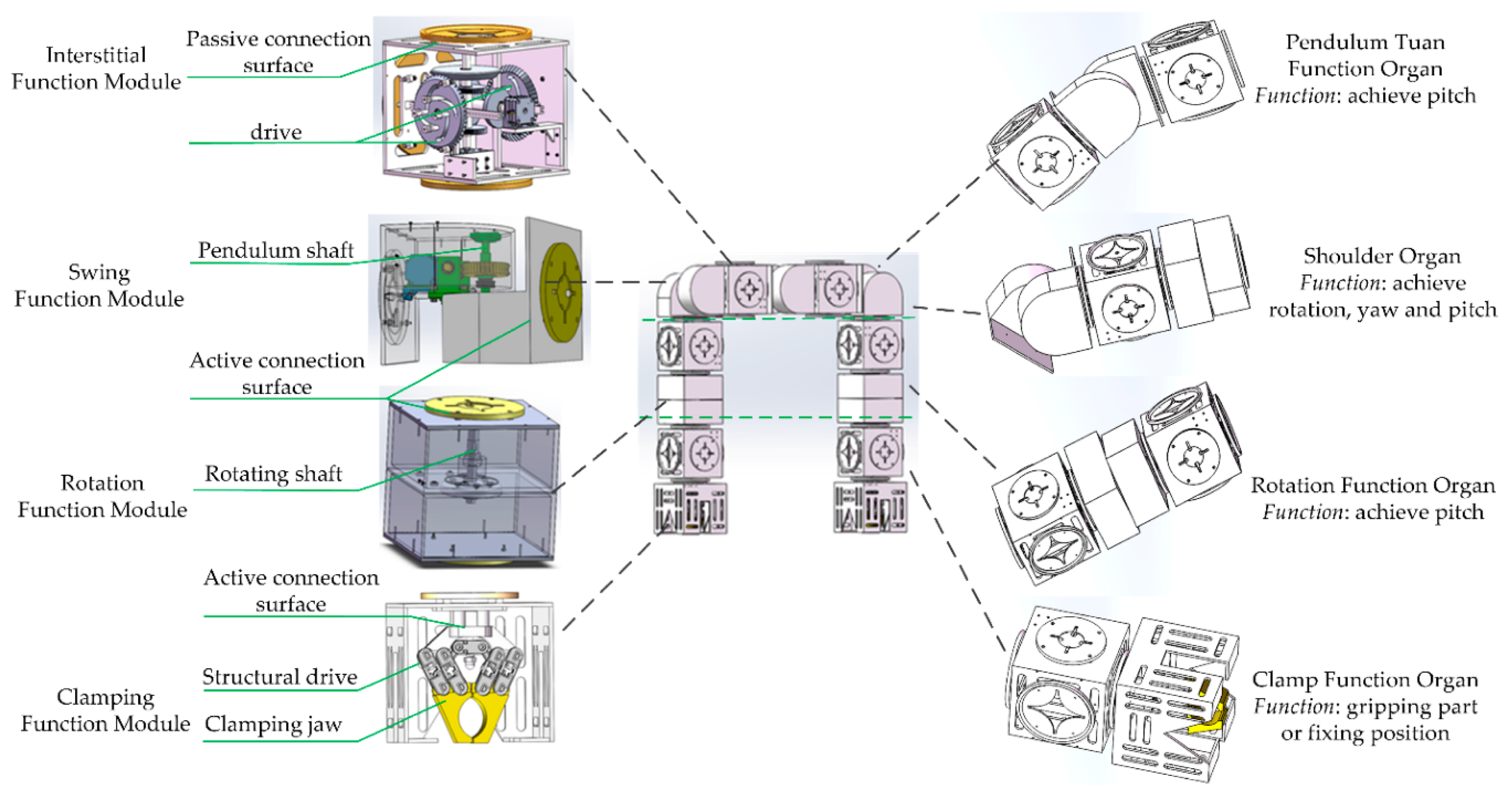
2.1. Design of the Robotic Function Module
2.2. Conformation Design Scheme for the Reconfigurable Robot
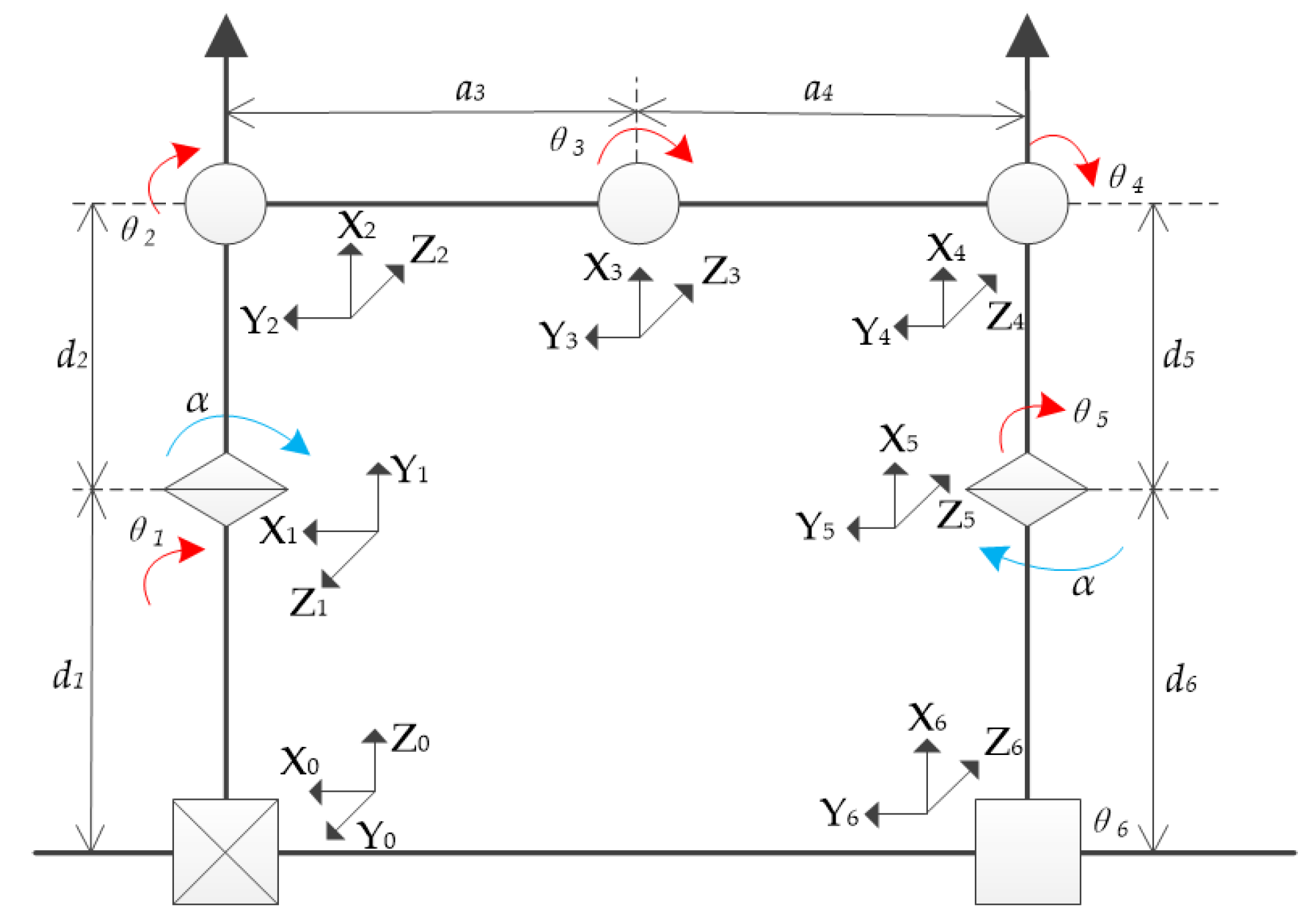
2.3. Kinematic Analysis
3. Research on Path Planning Based on Module Reconfiguration Platform
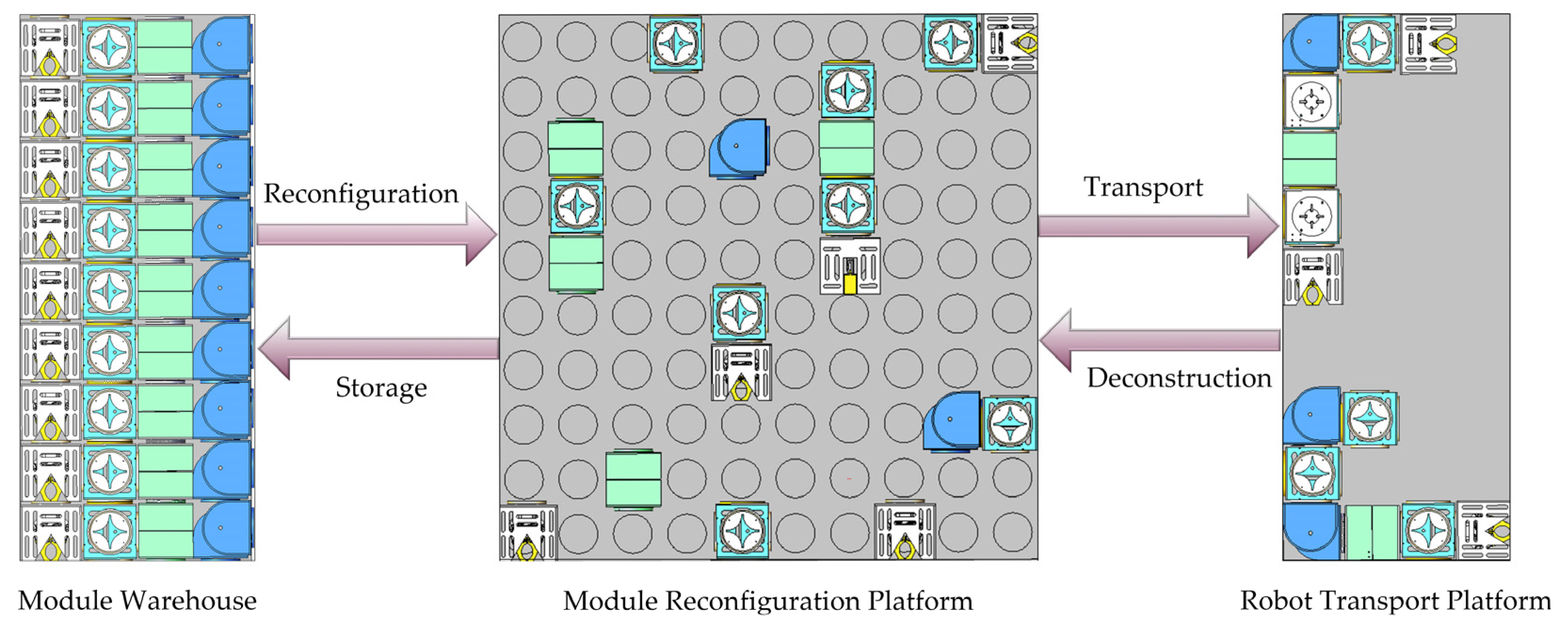
3.1. Building of the Module Reconfiguration Platform
3.1.1. Reconfiguration Platform Introduction
3.1.2. Mathematical Model of the Reconfiguration Platform
- (1)
- The movement space of modules is a two-dimensional environment.
- (2)
- Define the module’s movement step; the module moves one grid distance at a time, sets the module’s standard length to 200 mm, uniform motion for “v = 0.2 m/s”.
- (3)
- The coordinate of the module in the grid map is the center point of the grid.
- (1)
- Definition of the motion conditions: the reconfiguration function module is specified to carry out two-dimensional plane motion in the reconfiguration platform for the four directions of front, back, left, and right. The module moves in a certain direction if it meets the defined requirements.where: the “” indicates the functional module moves to the “step a”; and indicate the horizontal and vertical coordinates of the module at the “step a“.
- (2)
- Definition of the stop motion conditions: It is stipulated that the reconfiguration function module stops motion only when it moves to the target position. The condition for determining the module to stop is:that is: when the functional module moves from step “ ” to step “” with 0 step, the functional module remains stationary and the module reaches the target position.
3.2. Module Reconfiguration Campaign Definition
3.2.1. Mobile Priority for Functional Modules
- (1)
- When different modules are selected, the priority order of the modules is clamping function module, rotation function module, swing function module, interstitial function module.
- (2)
- If two modules are at the same priority level, the criteria for judging the priority level of the two modules is the distance for the module moves in the grid, and the module that moves farther away has a priority in choosing the path.
- (3)
- If the two modules move the same distance and have the same priority level, the functional module that has participated in robotic deconstruction has a higher priority than the module in the reconfiguration bin.
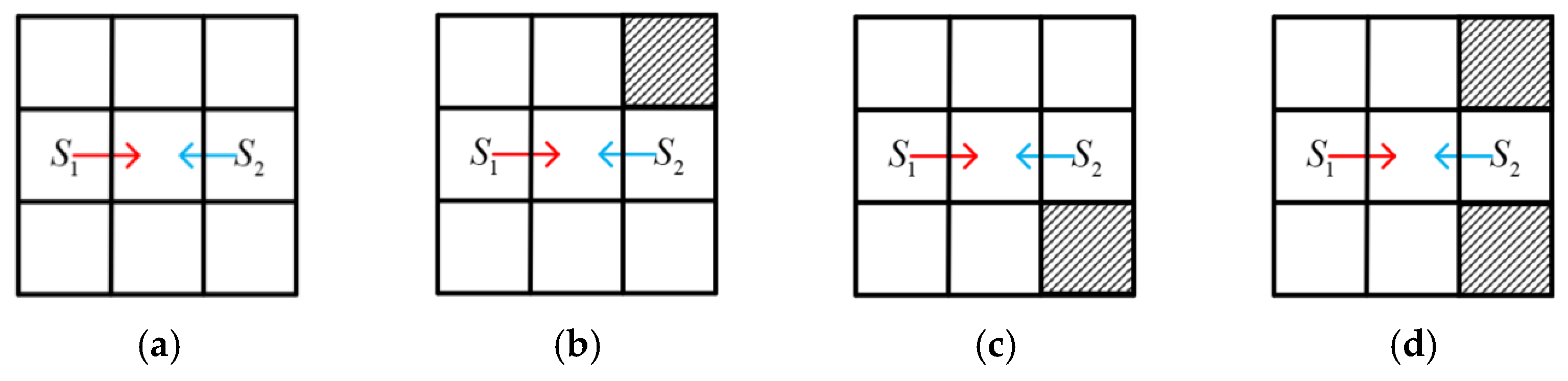
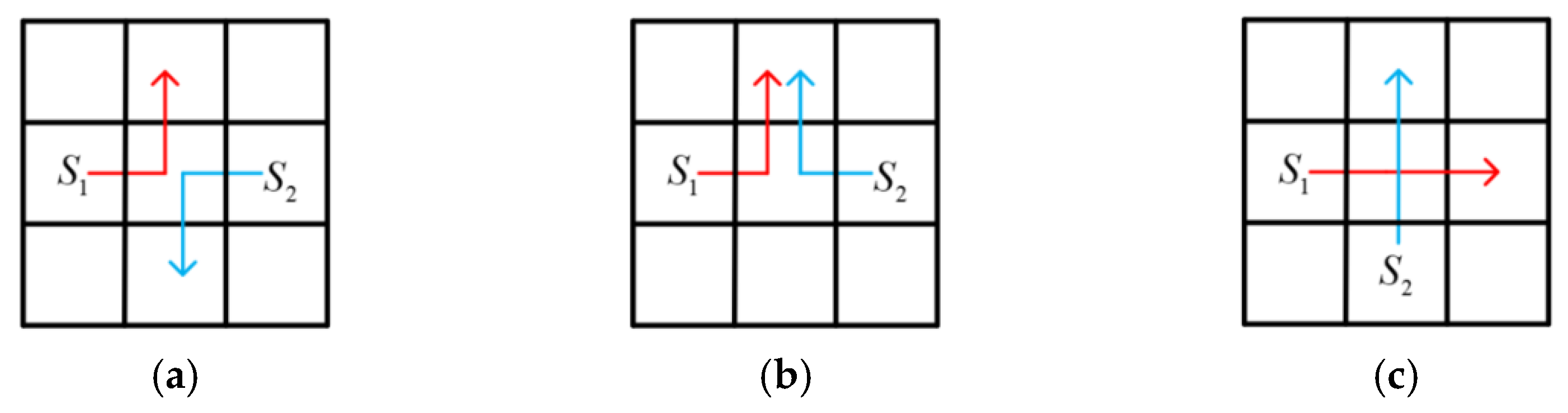
3.2.2. Establishment and Solution of the Functional Module Collision Avoidance Model
3.3. Modular Path Planning Based on Optimal Ant Colony Optimization
3.3.1. Ant Colony Optimization
- 1.
- Probability of state transferwhere “” is the transfer probability of the ant “k” from node “i” to node “j” at time “t”. The larger the value, the greater the probability that the ant chooses path “I → j”; “” is the pheromone concentration of the path at a time “t”; “” is the heuristic function; “α” and “β” are the pheromone and the desired heuristic factor, respectively; “” is the total amount of information from node “i” to target node “s”; “” is the value of the desired heuristic function from node “i” to target node “s”; “A” is the set of nodes that the ant “k” is allowed to select the next one.
- 2.
- Pheromone concentration
- 3.
- Forbidden table
3.3.2. Optimal ant Colony Algorithm Design
- 1.
- Set non-uniformly distributed initial pheromones
- 2.
- Design of the heuristic function
- (1)
- Distance heuristic factor
- (2)
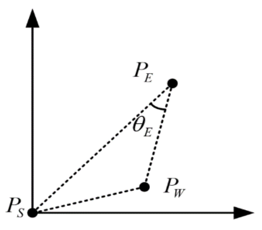
- Target pinch angle heuristic factor
- 3.
- Update pheromone
- 4.
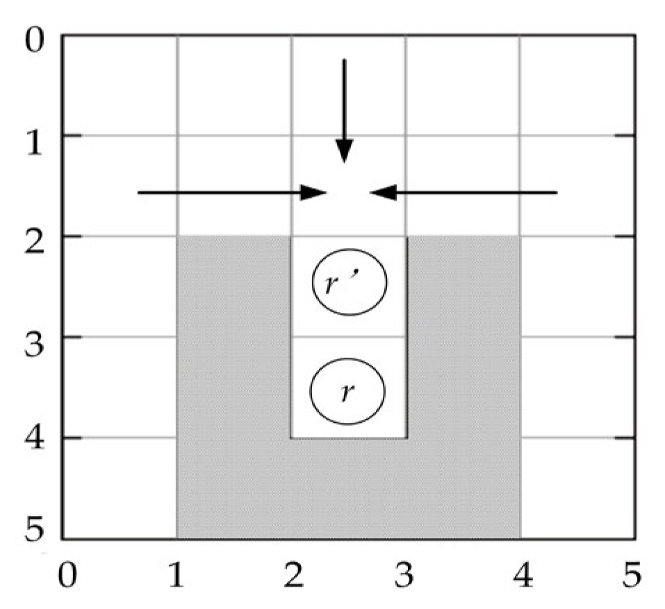
- Deadlock avoidance strategies
- 5.
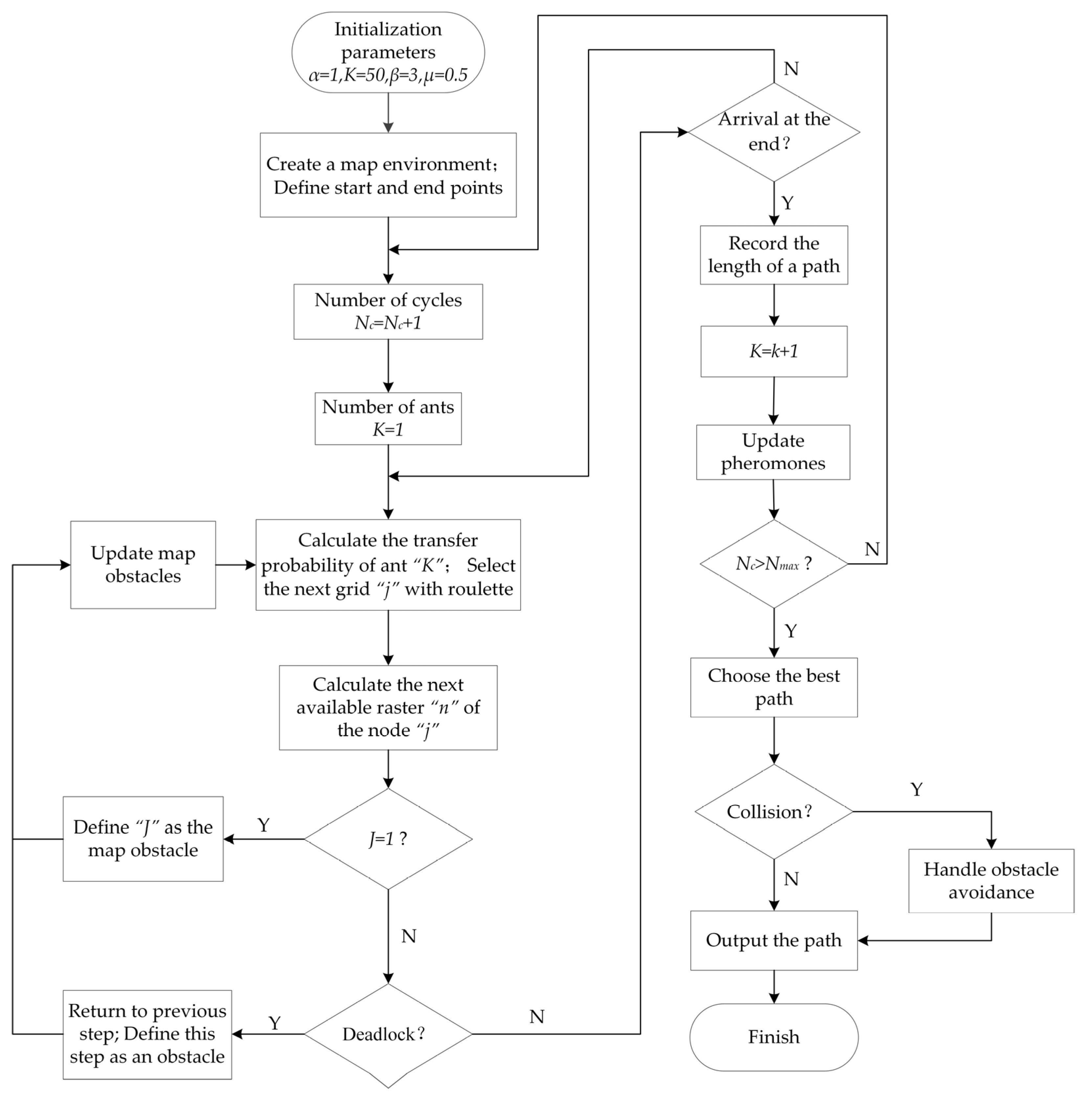
- Algorithmic steps
- -
- Step 1: Parameter initialization: set α = 1, K = 50, β = 3, μ = 0.5;
- -
- Step 2: Create the map environment and define the start and endpoints;
- -
- Step 3: Set the number of cycles: Nc = Nc + 1;
- -
- Step 4: Initialize the number of ants: K = 1;
- -
- Step 5: Calculate the transfer probability of the ant ”k”, and select the next moveable grid point “j” of the ant using the roulette wheel method;
- -
- Step 6: Calculate the next selectable grid point “n” of grid “j”;
- -
- Step 7: Determine “n = 1?”. If yes, define raster point “j” as an obstacle raster and update the map obstacle and return to step 5; otherwise, it will determine if the deadlock condition can be reached;
- -
- Step 8: Determine whether the deadlock condition is satisfied? If it satisfies, returning to the previous step “r − 1” and defining this step “r” as an obstacle, subsequently updating the map obstacle and returning to step 5; if it is not satisfied, determining whether ant “K (K = 1, 2,…, k)” reaches the final target point;
- -
- Step 9: Determine whether the ant reaches the endpoint? If the final target point is reached, recording the path length, otherwise returning to step 5;
- -
- Step 10: Set the number of ants: “K = k + 1”;
- -
- Step 11: Update the pheromone;
- -
- Step 12: Determine “Nc > Nmax?” if yes, choose the best path; otherwise returning to step 3;
- -
- Step 13: Determine whether the path generates collision? If yes, output the path after dealing with obstacles; otherwise, outputting the path directly;
- -
- Step 14: Finish.
4. Simulation and Analysis of Path Planning for Module’s Reconfiguration
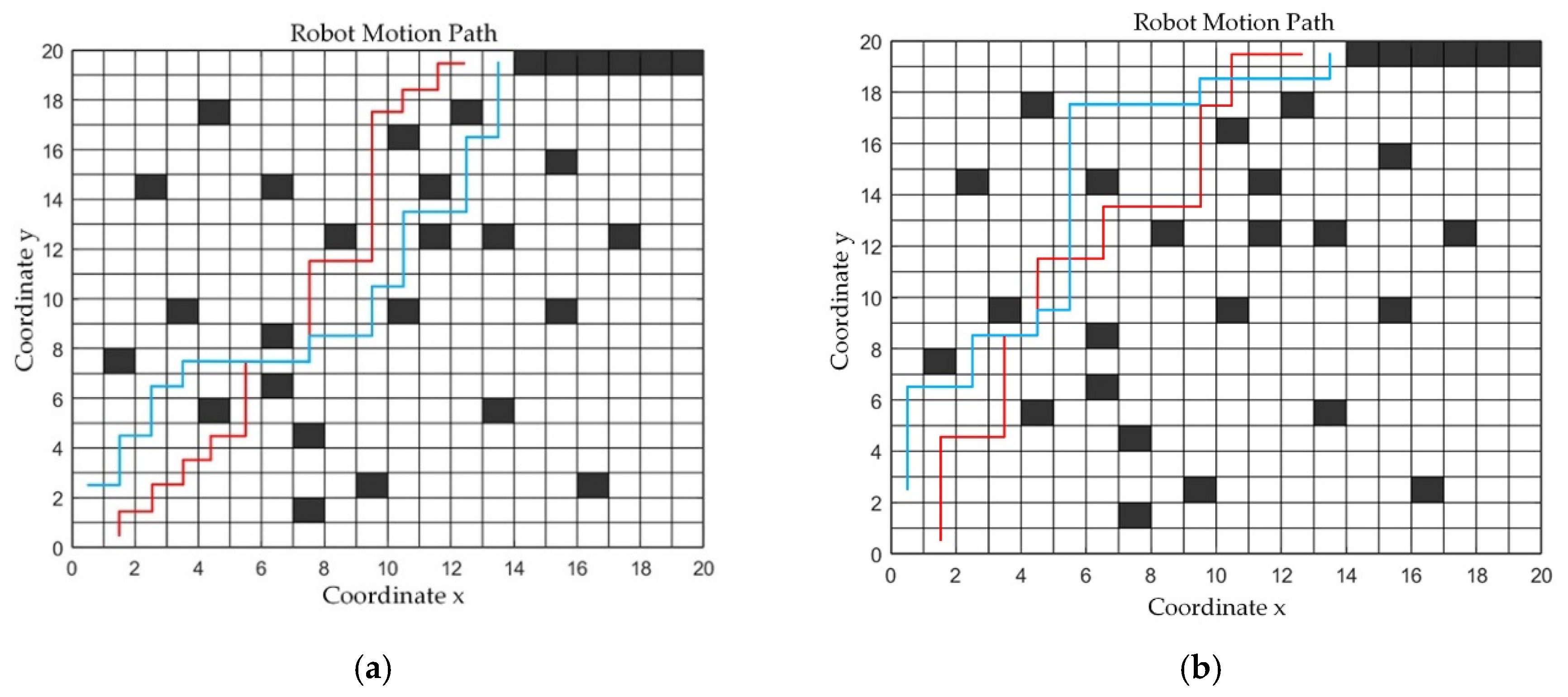
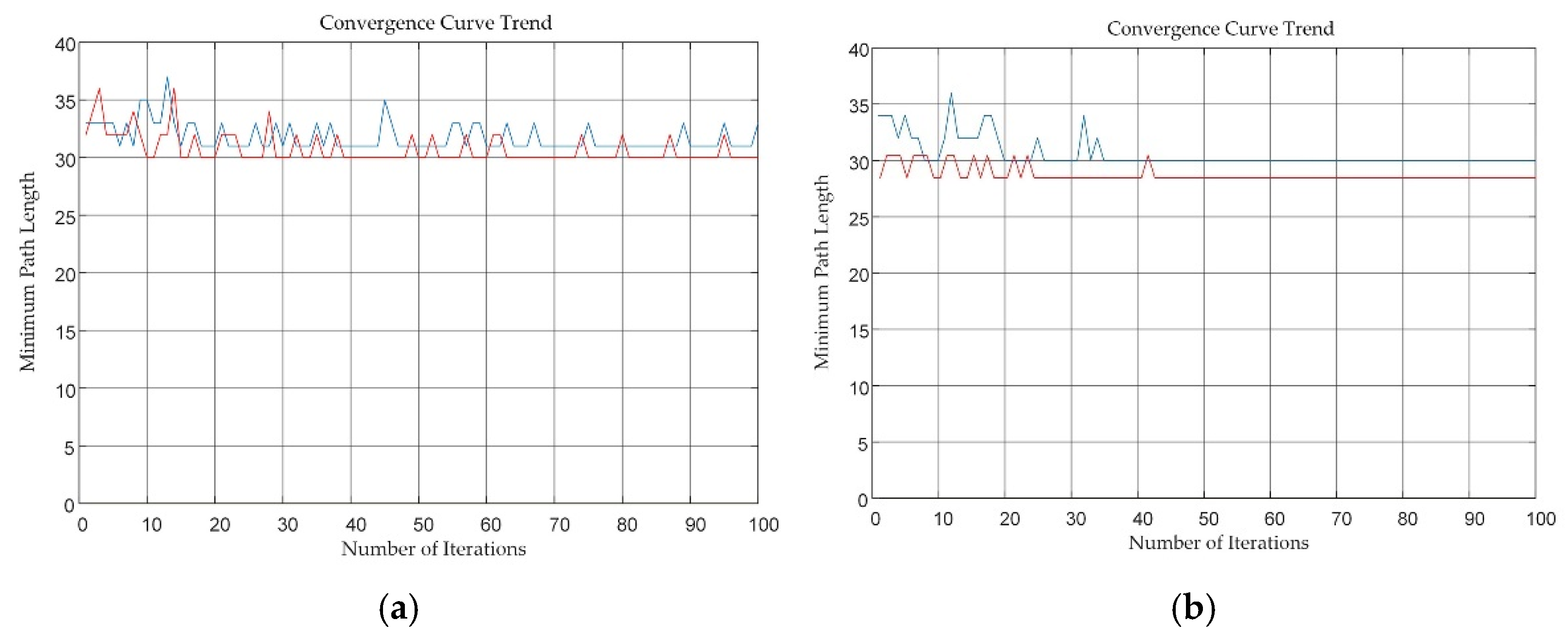
4.1. Reconfiguration Path Simulation Experiment
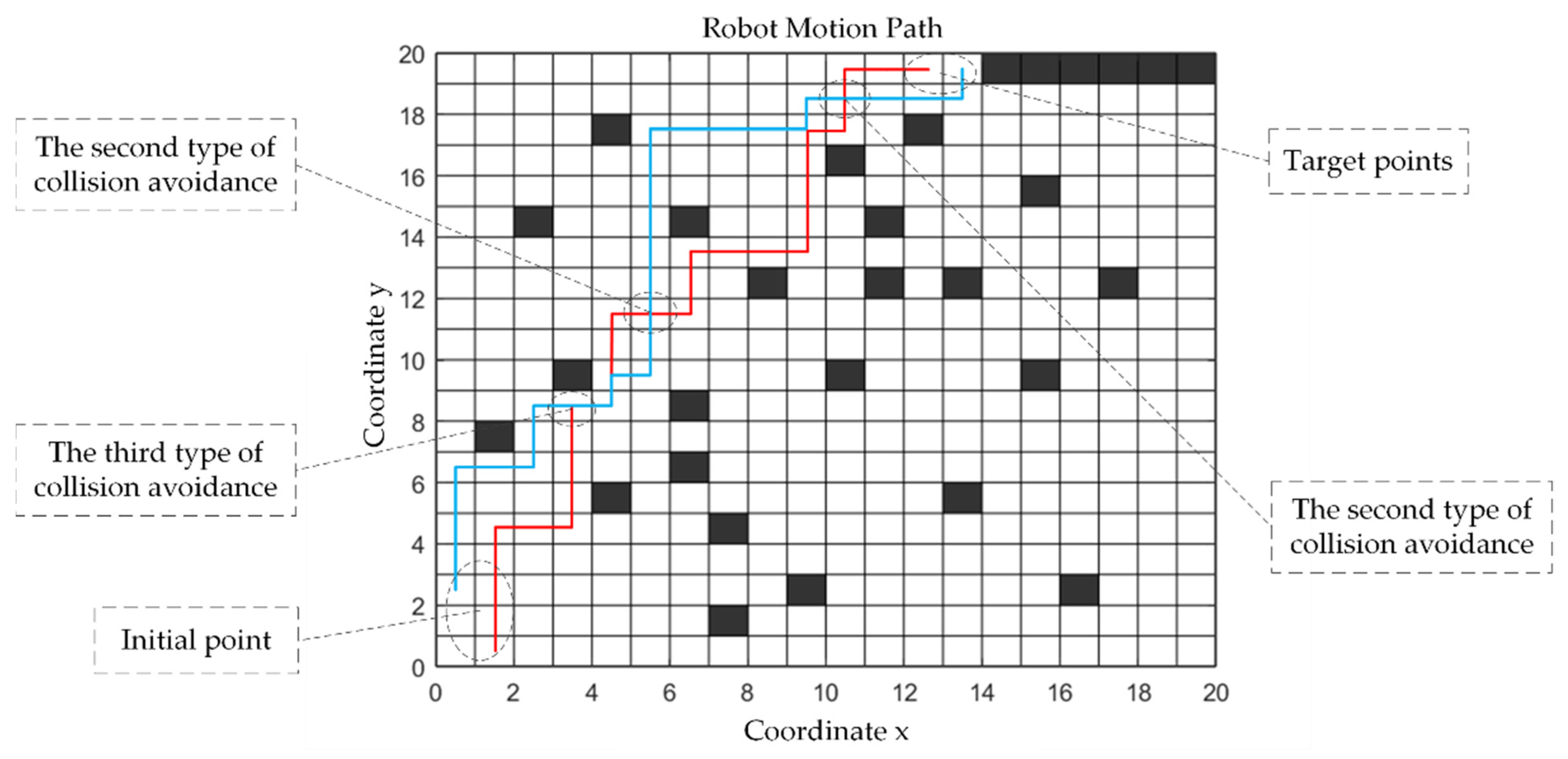
4.2. Collaborative Collision Analysis of Modules
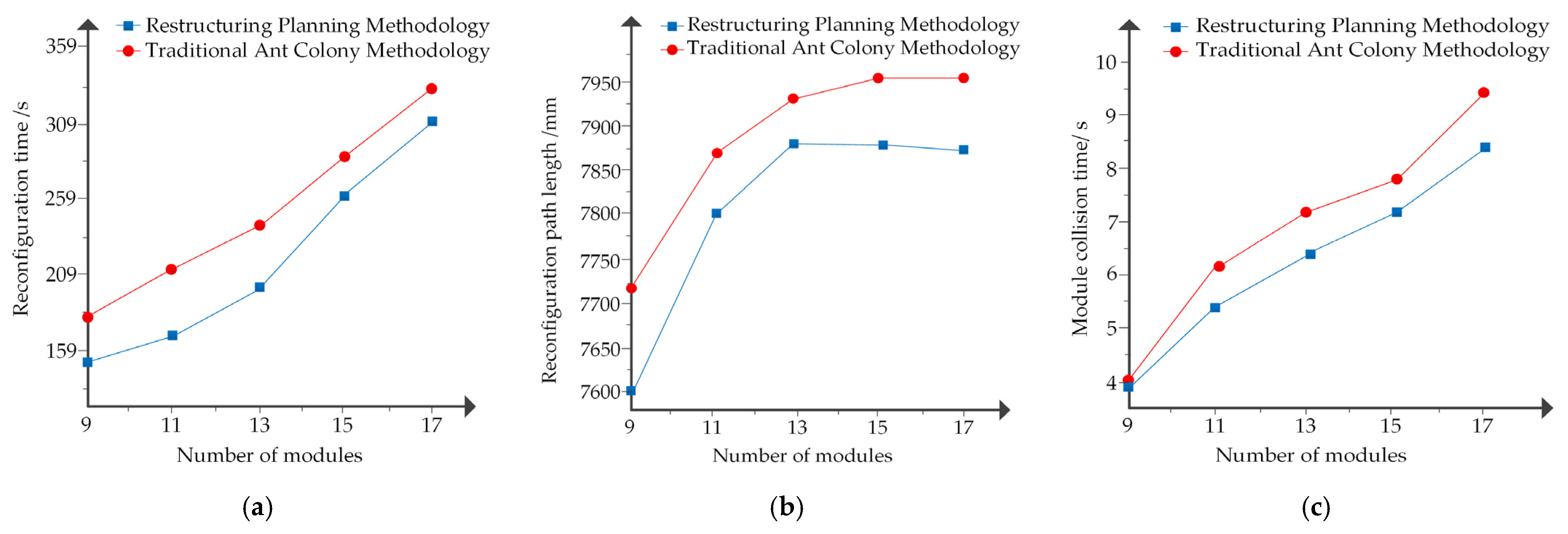
4.3. Module Reconfiguration Platform Planning Efficiency Analysis
5. Conclusions
- (1)
- In this paper, the configuration design of different reconfigured robotic configurations is based on the multilevel theory of mechanical modules. A kinematic analysis based on a fully functional robot is performed to establish the D-H parameters of the robot, which lays the mathematical foundation for the later paper.
- (2)
- We perform the construction and mathematical model description of the module reconfiguration platform and define the movement priority and collision avoidance guidelines for modules in the reconfiguration platform. An innovative path planning method based on the module reconfiguration platform is proposed to ensure that the robot can reconfigure its configuration according to the requirements of different operations.
- (3)
- Simulation verification and analysis of the proposed module’s reconfiguration path planning method in this paper. MATLAB simulates the cooperative path planning of two different functional modules to verify the rationality of the obstacle avoidance criterion and collision-free path planning. In addition, we analyze the collaborative planning efficiency of the reconfigured platform based on the configurations with different DOF and finally verify the advantages of the module reconfiguration planning method over the traditional ant colony algorithms through various aspects.
- The design of a robotic configuration scheme can also fully consider the advantages of parallel mechanisms or series-parallel hybrid mechanisms to improve the flexibility of the robotic configuration.
- This article considers the reconfiguration path planning research in the two-dimensional plane, and additionally, the obstacle avoidance and path planning research in the three-dimensional environment should also be considered.
- Research the module’s control strategy and integrate multiple algorithms to fully use the advantages of different algorithms and effectively improve reconfiguration efficiency.
Author Contributions
Funding
Institutional Review Board Statement
Informed Consent Statement
Data Availability Statement
Conflicts of Interest
References
- Liu, D.Y. Research on Reconfigurable Modular Robot Docking and Combination Strategy. Master’s Thesis, Shandong University, Jinan, China, 2020. (In Chinese). [Google Scholar]
- Gao, X.W. An analysis of industrial robots in intelligent manufacturing. Intern. Combust. Engine Parts 2021, 20, 199–200. [Google Scholar] [CrossRef]
- Christensen, D.J.; Schultz, U.P.; Stoy, K. A distributed and morphology-independent strategy for adaptive locomotion in self-reconfigurable modular robots. Robot. Auton. Syst. 2013, 61, 1021–1035. [Google Scholar] [CrossRef] [Green Version]
- Chu, K.D.; Hossain, S.G.M.; Nelson, C.A. Design of a four-DOF modular self-reconfigurable robot with novel gaits. In Proceedings of the ASME 2011 International Design Engineering Technical Conferences & Computers and Information in Engineering Conference, Washington, DC, USA, 28–31 August 2011; pp. 1–8. [Google Scholar]
- Gao, S.Q.; Guo, S.G.; Xing, D.D. Research on self-reconfiguring modular robot. Comput. CD Softw. Appl. 2013, 1, 63–64. [Google Scholar]
- Fukuda, T. Approach to the Dynamically Reconfigurable Robotic System. J. Intell. Robot. Syst. 1988, 1, 55–72. [Google Scholar] [CrossRef]
- Castano, A.; Behar, A.; Will, P.M. The Conro modules for reconfigurable robots. IEEE/ASME Trans. Mechatron. 2002, 7, 403–409. [Google Scholar] [CrossRef] [Green Version]
- Rubenstein, M.; Payne, K.; Will, P. Docking among independent and autonomous CONRO self-reconfigurable robots. In Proceedings of the IEEE International Conference on Robotics and Automation, New Orleans, LA, USA, 26 April–1 May 2004; pp. 2877–2882. [Google Scholar]
- Acaccia, G.; Bruzzone, L.; Razzoli, R. A modular robotic system for industrial applications. Assem. Autom. 2008, 28, 151–162. [Google Scholar] [CrossRef]
- Zhang, S.C.; Pu, J.X.; Si, Y.N.; Sun, L. Path planning for mobile robot using an enhanced ant colony optimization and path geometric optimization. Int. J. Adv. Robot. Syst. 2021, 18, 3. [Google Scholar] [CrossRef]
- Guo, P.; Zhang, J.W.; Rong, F. Application of ant colony algorithm in unmanned park tour route. Mod. Electron. Tech. 2019, 42, 149–152. [Google Scholar]
- Zhang, X.L.; Yang, Y.X.; Xie, Y.C. An improved ant colony algorithm for robot path planning. Comput. Eng. Appl. 2020, 56, 29–34. [Google Scholar]
- Li, Y.; Ji, J.N.; Shen, J.L.; Su, R. A path planning method for mobile robots based on improved ant colony algorithm. J. Nanjing Univ. Inf. Sci. Technol. 2021, 13, 298–303. [Google Scholar] [CrossRef]
- Jiang, M.; Wang, F.; Ge, Y.; Sun, L.L. Research on path planning of mobile robot based on improved ant colony algorithm. Chin. J. Sci. Inst. 2019, 40, 113–122. [Google Scholar] [CrossRef]
- Deng, H.Y. Comparative Study of Ant Colony Algorithm, Genetic Algorithm and the Fusion of Both in TSP Application. Master’s Thesis, Shanxi Normal University, Xi’an, China, 2017. (In Chinese). [Google Scholar]
- Tao, Y.; Gao, H.; Ren, F.; Chen, C.Y.; Wang, T.M.; Xiong, H.G.; Jiang, S. A Mobile Service Robot Global Path Planning Method Based on Ant Colony Optimization and Fuzzy Control. Appl. Sci. 2021, 11, 3605. [Google Scholar] [CrossRef]
- Niu, L.H.; Ji, N.P. Research on robot path planning problem based on improved ant colony algorithm. Microprocessors 2020, 41, 37–40. [Google Scholar]
- Li, S.D.; You, X.M.; Liu, S. A dual ant-state ant colony algorithm combining the dynamic grading of ABC algorithm. Comput. Eng. Appl. 2020, 56, 37–46. [Google Scholar]
- Anh, V.L.; Veerajagadheswar, P.; Vinu, S. Modified A-Star algorithm for efficient coverage path planning in tetris inspired self-reconfigurable robot with integrated laser sensor. Sensors 2018, 18, 2585. [Google Scholar] [CrossRef] [Green Version]
- Sun, J.B.; Liu, G.L.; Tian, G.H. Smart obstacle avoidance using a danger index for a dynamic environment. Appl. Sci. 2019, 9, 1589. [Google Scholar] [CrossRef] [Green Version]
- Liang, J.H.; Lee, C.H. Efficient collision-free path planning of multiple mobile robots system using efficient artificial bee colony algorithm. Adv. Eng. Softw. 2015, 79, 47–56. [Google Scholar] [CrossRef]
- Qi, R.L.; Zhou, W.J.; Liu, J.G.; Zhang, W.; Lei, X. Obstacle avoidance trajectory planning for gaussian motion of robot based on probability theory. J. Mech. Eng. 2017, 53, 92–100. [Google Scholar] [CrossRef]
- Su, J.B.; Xie, W.L. Motion planning and coordination for robot systems based on representation space, transactions on systems. IEEE Trans. Syst. Man Cyb. 2011, 41, 248–260. [Google Scholar] [CrossRef] [PubMed]
- Zhang, H.B. Research on the Design and Reconfiguration Strategy of Space Truss in-Orbit Assembly Robot; Harbin Institute of Technology: Harbin, China, 2020. [Google Scholar]
- Liu, K.Y.; Chen, M.; Fei, Y.Q. Reconfiguration strategy for tandem modular robots. High Tech. Lett. 2019, 29, 995–1002. [Google Scholar]
- Lin, J.Z.; Ye, C.C.; Yang, J.X.; Zhao, H.; Ding, H.; Luo, M. Contour error-based optimization of the end-effector pose of a 6 degree-of-freedom serial robot in milling operation. Robot. Comput.-Integr. Manuf. 2022, 73, 102257. [Google Scholar] [CrossRef]
- Ma, L.; Zhao, S.D. Analysis of combined symmetry concept system and application of mechanical structure. Mod. Manuf. Technol. Equip. 2018, 4, 45–47. [Google Scholar]
- Zuo, Z.H. Research on Fast Modeling of Kinematics and Dynamics of Modular Robotic Arm. Master’s Thesis, Beijing University of Posts and Telecommunications, Beijing, China, 2015. (In Chinese). [Google Scholar]
- Song, W.G. Fundamentals of Robotics; Metallurgical Industry Press: Beijing, China, 2015; pp. 61–66. [Google Scholar]
- Zhu, Y.; Zhu, L.C.; Long, Y.; Luo, J.Q. The Wolf pack assignment rule based on ant colony algorithm and the path planning of scout ants in complex raster diagra. J. Phys. Conf. Ser. 2021, 1, 1732. [Google Scholar] [CrossRef]
- Li, H.; Zang, L.; Gan, L. Path search for guessing symbolic execution based on ant colony algorithm. Comput. Sci. 2018, 45, 145–150. [Google Scholar]
- Wang, Y. Research on the optimization method of air logistics distribution path based on ant colony algorithm. Inf. Technol. 2021, 11, 76–80. [Google Scholar]
- Liu, Y. Robot path planning method based on improved potential field and ant colony algorithm. Comput. Simul. 2021, 38, 355–360. [Google Scholar]


| DOF | 3-D Model | Components | Characteristics |
|---|---|---|---|
| Three | 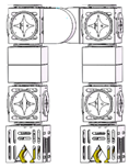 | 2 rotating modules 1 swing module 2 clamping modules 4 interstitial modules | It has low freedom for simple grasping or climbing. |
| Four | 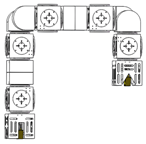 | 2 rotating modules 2 swing modules 2 clamping modules 5 interstitial modules | With a certain degree of flexibility, and it can complete the position adjustment. |
| Five | 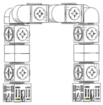 | 3 rotating modules 2 swing modules 2 clamping modules 6 interstitial modules | High flexibility for most basic tasks. |
| Six |  | 2 rotating modules 4 swing modules 2 clamping modules 7 interstitial modules | Meet the needs of free space for installation in any position |
| Seven |  | 2 rotating modules 5 swing modules 2 clamping modules 8 interstitial modules | Consider the advantages of redundant motility |
| Joint | Turn α | Length a | Offset d | Angle θ | Range |
|---|---|---|---|---|---|
| Module 1 | 0° | 0 | −180~180° | ||
| Module 2 | 90° | 0 | 0 | −90~90° | |
| Module 3 | 0° | 0 | −90~90° | ||
| Module 4 | 0° | 0 | −90~90° | ||
| Module 5 | −90° | 0 | 0 | −180~180° | |
| Module 6 | 0° | 0 | 0° |
| Parameters | Traditional Ant Colony Optimization | Optimized Ant Colony Optimization |
|---|---|---|
| Ant population | 50 | 50 |
| Iteration number | 100 | 100 |
| Pheromone inspired factor | 1 | 1 |
| Expectation heuristic factor | 3 | 3 |
| Pheromone evaporation factor | ||
| Distance heuristic factor | ||
| Nodal perspective heuristic factor | / | |
| Initial pheromone | Uniform distribution | Non-uniform distribution |
| Deadlock handling | / | Fallback strategy |
| DOF | Three | Four | Five | Six | Seven |
|---|---|---|---|---|---|
| Total Modules | 9 | 11 | 13 | 15 | 17 |
| Motion Modules | 5 | 6 | 7 | 8 | 9 |
| Interstitial Modules | 4 | 5 | 6 | 7 | 8 |
Publisher’s Note: MDPI stays neutral with regard to jurisdictional claims in published maps and institutional affiliations. |
© 2022 by the authors. Licensee MDPI, Basel, Switzerland. This article is an open access article distributed under the terms and conditions of the Creative Commons Attribution (CC BY) license (https://creativecommons.org/licenses/by/4.0/).
Share and Cite
Dai, Y.; Xiang, C.-F.; Liu, Z.-X.; Li, Z.-L.; Qu, W.-Y.; Zhang, Q.-H. Modular Robotic Design and Reconfiguring Path Planning. Appl. Sci. 2022, 12, 723. https://doi.org/10.3390/app12020723
Dai Y, Xiang C-F, Liu Z-X, Li Z-L, Qu W-Y, Zhang Q-H. Modular Robotic Design and Reconfiguring Path Planning. Applied Sciences. 2022; 12(2):723. https://doi.org/10.3390/app12020723
Chicago/Turabian StyleDai, Ye, Chao-Fang Xiang, Zhao-Xu Liu, Zhao-Long Li, Wen-Yin Qu, and Qi-Hao Zhang. 2022. "Modular Robotic Design and Reconfiguring Path Planning" Applied Sciences 12, no. 2: 723. https://doi.org/10.3390/app12020723
APA StyleDai, Y., Xiang, C.-F., Liu, Z.-X., Li, Z.-L., Qu, W.-Y., & Zhang, Q.-H. (2022). Modular Robotic Design and Reconfiguring Path Planning. Applied Sciences, 12(2), 723. https://doi.org/10.3390/app12020723