Prediction of Solar Irradiance over the Arabian Peninsula: Satellite Data, Radiative Transfer Model, and Machine Learning Integration Approach

Abstract

Data from a moderate resolution imaging spectroradiometer instrument onboard the Terra satellite along with a radiative transfer model and a machine learning technique were integrated to predict direct solar irradiance on a horizontal surface over the Arabian Peninsula (AP). In preparation for building appropriate residual network (ResNet) prediction models, we conducted some exploratory data analysis (EDA) and came to some conclusions. We noted that aerosols in the atmosphere correlate with solar irradiance in the eastern region of the AP, especially near the coastlines of the Arabian Gulf and the Sea of Oman. We also found low solar irradiance during March 2016 and March 2017 in the central (~20% less) and eastern regions (~15% less) of the AP, which could be attributed to the high frequency of dust events during those months. Compared to other locations in the AP, high solar irradiance was recorded in the Rub Al Khali desert during winter and spring. The effect of major dust outbreaks over the AP during March 2009 and March 2012 was also noted. The EDA indicated a correlation between high aerosol loading and a decrease in solar irradiance. The analysis showed that the Rub Al Khali desert is one of the best locations in the AP to harvest solar radiation. The analysis also showed the ResNet prediction model achieves high test accuracy scores, indicated by a mean absolute error of ~0.02, a mean squared error of ~0.005, and an R² of 0.99.

1. Introduction

Renewable energy technologies, including photovoltaic (PV) technology, could play a significant role in supplying rising global energy demand with low environmental impacts [1]. The sun generates an abundant and unbounded energy resource but is not evenly distributed over the globe. To maximize direct normal irradiance (DNI), PV cells are preferably installed at low latitude within 30° S–30° N. For example, the Al Rub’ al Khali (The Empty Quarter) desert (21.09° N) in the Arabian Peninsula (AP) (~40° E–60° E, ~14° N–30° N), see Figure 1, and the Sahara Desert (SD) in Africa (23.4° N) receive 5.26 and 6.35 kWhm⁻²day⁻¹, respectively [2]. The DESERTEC project [3] showed that the desert sun could provide the Middle East and North Africa (MENA) countries with affordable, reliable, and sustainable energy, reduce emissions and powering desalination plants to supply fresh water to the MENA countries. In Saudi Arabia, the 300 MW Sakaka IPP PV solar project is another project that represents the first-ever utility-scale renewable energy project under the National Renewable Energy Program of Saudi Arabia [4]. The plant will cover an area of six square kilometers with an investment of US $302 million. This project is the first of a series of projects under the Saudi National Renewable Energy Program, which aims to produce 9.5 GW of renewable energy by 2023.

Even though deserts could provide the right environment for harvesting solar energy, optimizing the tilt angle of PV cells and understanding surrounding environmental conditions can increase the efficiency of the cells [5,6,7]. Many studies report a loss in the energy yield, the grid reliability, and the stability of the PV cells due to various environmental impacts in deserts [8]. Numerous studies [9,10] have investigated PV-cell power-transmission losses due to adverse weather conditions such as wind speed/direction, temperature, relative humidity, and the frequency of dust storms. Dust accumulation on PV cells (known as the soiling effect) is also known to have a significant impact on power-yield loss due to scattering effects and absorption of the incident light by constituents in the atmosphere [11].

Atmospheric aerosols can directly/indirectly influence the global radiation budget and the earth’s climate by modifying its energy balance. Nevertheless, the uncertainty of aerosol impact on the global radiation budget significantly exceeds that of any other climate-forcing parameter [12]. This is due to the inhomogeneous concentration of aerosols and the spatial–temporal variability of their physical and chemical properties [13]. Reducing the uncertainty of aerosol impact on solar radiation is essential in the assessment of PV-system efficiency.

Solar radiation is strongly impacted by the aerosols’ physical and chemical properties, such as particles’ shape, size, altitude, and chemical composition [14]. Depending on their absorption and scattering properties, aerosols may reduce DNI. The impact of aerosols on solar radiation is even more significant over climatically sensitive regions like the AP, which hosts one of the largest deserts in the world (i.e., Al Rub’ al Khali). The AP is also the home of the An-Nafud desert, where sand dunes often exceed a height of 30 m. This vast desert environment makes the AP one of the main terrestrial sources of dust aerosols. During transportation over industrial and/or city atmospheres, these aerosols may be coagulated with anthropogenic emissions originating from the petrochemical industry and mega infrastructures [15,16,17,18]. The mean value of the aerosol optical depth (AOD), a good indicator of the atmospheric aerosol concentration, has recently been measured at 0.38 over the AP [19], a value 2.4 times larger than the corresponding global mean of 0.17 [20]. Nevertheless, the mean value of the AOD over the AP is highly variable in space and time because of frequent dust storms and anthropogenic emissions [21]. The aerosol radiative impacts over the AP have been investigated by many researchers in recent decades [22,23,24,25]. Nevertheless, more efforts are required to predict solar irradiance following the effects of natural and anthropogenic aerosols in different regions.

The prediction of solar irradiance lends itself to a form of time-series analysis. The values of solar irradiance are recorded in a sequence. This sequence follows a successive order controlled by the time in which each value was recorded. The generated sequence of time steps formulates time-series data. This format of data shapes the base of many applications such as stock-price forecasting, climate modeling, and transportation planning, to name few. Therefore, there has been considerable interest in time-series analysis, specifically with regard to time-series classification [26] and forecasting [27] tasks. Time-series classification categorizes time series in predefined classes, while forecasting the future values of time series reflects the closest recent values. The latter category, forecasting, represents the task considered here to predict solar irradiance. Tracing the different techniques used to solve prediction problems, the machine-learning (ML) techniques have provided the field with promising results. These results motivated us to investigate the applicability of such techniques to predict solar irradiance over the AP.

In this work, the radiative transfer model (RTM) [28,29] is integrated with one of the prominent ML models, i.e., residual network (ResNet) [30], to predict solar irradiance over the AP. Note that the work presented in this research effort represents an application of an existing ML model, and does not aim to improve the model or enhance its performance.

2. Theoretical Background

In this section, we mention some essential points related to ResNets and RTMs for predicting solar radiation at a location and depict the benefits of using satellite observations for this purpose. As a foundation for the paper, this background information ensures its comprehensiveness and completeness.

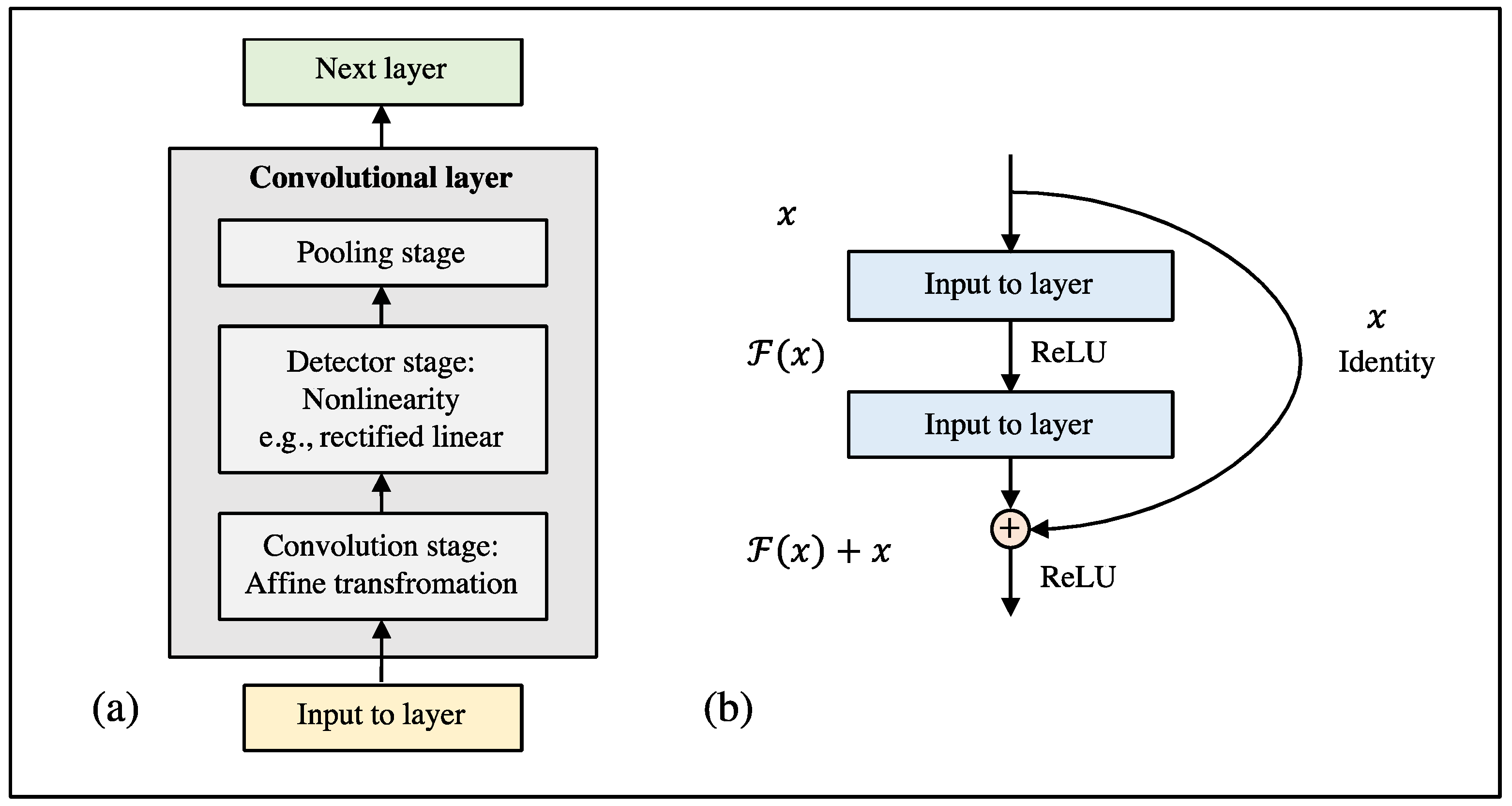
2.1. Residual Networks (ResNets)

Machine learning (ML) is an artificial intelligence technique that can be used to find the relationship between a set of input records and their related output if this is very difficult using explicit algorithms. This property of ML facilitates its use in many fields such as the one considered within this research, in which it will be utilized to predict solar irradiance considering earlier observed data of solar irradiance as time series. Many techniques have been utilized to predict solar irradiance. Some of these techniques are commonly used, such as the support-vector machine (SVM) and clustering by the k-nearest neighbor (k-NN), whereas others are rarely used, such as regression trees or similar methods (boosting, bagging, or random forest) [31]. The success of deep learning (DL), a branch of ML, in many fields has encouraged the trend of harnessing its efficiency to model solar radiation [14]. Artificial neural networks (ANNs) represent the building block of DL models and are specifically predominant in the events of time-series forecasting with nonlinear methods [26]. Different types of neurons lead to some recognizable neural networks. For instance, long short-term memory (LSTM) networks were proposed as a powerful approach for time-series forecasting with the potential to predict solar irradiance. It has turned out to be a promising technique when compared to other ML algorithms, with a proven track record in irradiance forecasting [32]. LSTM has also outperformed other algorithms such as the linear least-squares regression (LR) method and the ANN using the classical backpropagation algorithm (BPNN) [26]. Despite the notable performance offered by LSTM, such a network is known for its high computational complexity and increased need for memory. Therefore, a simpler model is required to offer equivalent results, while maintaining a lower cost. ResNets [30] are a special variant of deep feedforward convolutional neural networks (CNNs). Along with heavy batch normalization, ResNets are composed of blocks, each of which is in turn composed of convolutional layers. CNNs can extract features of temporal data and they are preferred to other networks, such as the recurrent neural networks (RNNs), if the data have a considerably short history. The blocks have internal residual skip connections that connect the blocks skipping a fixed sequence of layers within the block, hence the name residual block and residual network. Such residual skip connections, also known as gated units or gated recurrent units, are shortcut links that keep a knowledge transfer among the blocks. They have a strong similarity to the elements that contribute to the success of RNNs in sequence analysis utilizing an added value to the CNNs’ feature extraction capacities. Residual connections are supporting further analysis based on the previous copy of data as well as the features extracted at the previous convolutional layers. Figure 2a shows a typical convolution layer that contains a convolution stage, followed by a stage of activation, typically using rectified linear unit (ReLU) and then a pooling stage. Figure 2b shows an example of a residual block that is demonstrating a residual skip connection where the identity is transferred by skipping two layers. ResNets resolve the issues raised by the models discussed earlier, such as the requirement of high computational power and large storage. ResNets have also surpassed many other models when solving time-series problems [26]. Their performance has been compared by [26] to 8730 DL models that have been trained on 97 time-series datasets of both univariate and multivariate records. Their results showed that ResNet achieved higher performance for most time-series datasets, including those representing the type of data targeted in this work.

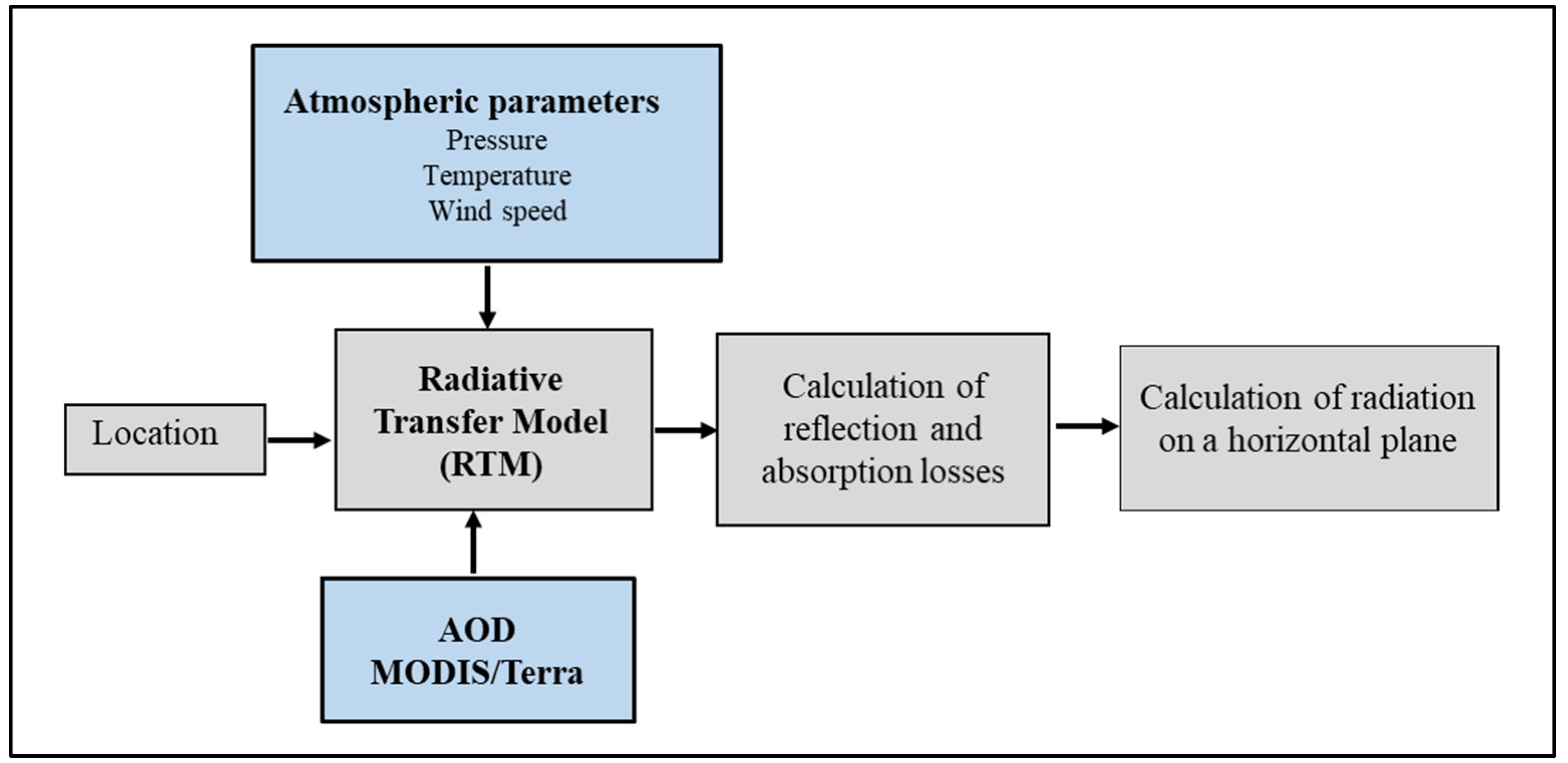
2.2. Radiative Transfer Model (RTM)

For estimating the aerosol impacts on solar radiation over the AP, a spectral RTM can be applied over the area; the structure of the model is depicted in Figure 3. The RTM employs a library of radiative transfer routines and programs (i.e., libRadtran) to estimate spectral flux in the VIS and UV bands of the spectrum [33]. The RTM calculates solar radiation fluxes with a resolution of 2.5° × 2.5° under both clear- and cloudy-sky conditions. Solar radiative fluxes are computed at 118 wavelengths in the range 0.2–1.0 $\mathsf{\mu }\mathrm{m}$and 10 spectral intervals in the range 1.0–10 $\mathsf{\mu }\mathrm{m}$ taking Rayleigh scattering, methane, carbon dioxide, water vapor, and ozone absorption into account [12,34,35,36]. Single-scattering albedo (SSA), absorption, scattering by aerosols and clouds at different altitudes are also considered [37].

Solar irradiance is calculated as the difference between solar flux with ($S{F}_{atm, w}$) and without ($S{F}_{atm, wo}$) the presence of aerosols:

$$DR{E}_{atm}= S{F}_{atm, w}-S{F}_{atm, wo}$$

$$DR{E}_{surf}= S{F}_{surf, w}-S{F}_{surf, wo}$$

where $DR{E}_{atm}$, $DR{E}_{surf}$represent the effect of aerosols on solar radiation within the atmosphere and near the earth’s surface, respectively.

The aerosol radiation budget (ARB) is another factor used to determine the effect of aerosols on solar radiation fluxes and is given by:

$$AR{B}_x=DR{E}_x/S{F}_{x, wo}$$

which is equivalent to:

$$AR{B}_x= S{F}_x/S{F}_{x, wo}$$

where the subscript x corresponds to “atm” or “surf”.

Based on the aerosol loading in the atmosphere as an input to the algorithm of Figure 3, we use the library of the RTM model to estimate DNI on a horizontal surface. The atmosphere is defined in the model through an input file that includes profiles of temperature, pressure, air density, ozone, carbon dioxide, nitrogen dioxide, oxygen, and water vapor provided by the World Weather Records (WWR) [38].

2.3. Moderate Resolution Imaging Spectroradiometer (MODIS)

The model input also includes the AOD and SSA retrieved from the MODIS instrument onboard the Terra satellite. The MODIS sensor has provided data on aerosol properties since its launch in 2000 [20,40]. MODIS/Terra provide the AOD product over land and water at 10-km resolution [20]. The AOD uncertainty is ±0.05 (±0.2 AOD) over land and ±0.03 (±0.05 AOD) over ocean; the uncertainty in the fine fraction monthly mean AOD is about 20% [20,41]. MODIS retrieves the AOD over vegetated areas at three visible channels (0.47, 0.55, and 0.66 $\mathsf{\mu }\mathrm{m}$) with an accuracy of ±0.05 [40]. In addition, it also provides surface reflectance over land in VIS (0.3–0.7 $\mathsf{\mu }\mathrm{m}$), IR (0.7–5.0 $\mathsf{\mu }\mathrm{m}$), and broadband (0.3–5.0 $\mathsf{\mu }\mathrm{m}$), as well as at 0.47, 0.55, 0.67, 0.86, 1.24, and 2.1 $\mathsf{\mu }\mathrm{m}$ [42]. The MODIS global albedo retrievals have a spatial resolution of 0.05° in a geographic (latitude /longitude) projection [43]. The effect of clouds on albedo is not considered in this study. The diurnal surface albedo variation, which may lead to an uncertainty of about 5% in the monthly average values, is also neglected in this study.

The Deep Blue (DB) product is used over desert areas rather than the standard AOD product, as it is retrieved using the dark-target approach in the band 2.1–3.8 $\mathsf{\mu }\mathrm{m}$ [44]. The uncertainties of the DB product are reported to be around 25–30% [45]. The most recent 3-km high-resolution MODIS Collection 6 dataset release Level-3 data (https://giovanni.gsfc.nasa.gov/giovanni/, accessed on 1 July 2021) is used in this study [46]. The use of spectral aerosol optical properties along with a detailed spectral RTM in the present study ensures the calculation of quality aerosol DRE values, as has been shown in previous studies [35,37]; the aerosol radiative effects are quite sensitive to the spectral dependence of the aerosol optical properties.

3. Model Setup and Data Collection

In this section, we discuss the integration of MODIS and RTM with the ResNet model to predict DNI on a horizontal surface over the study region.

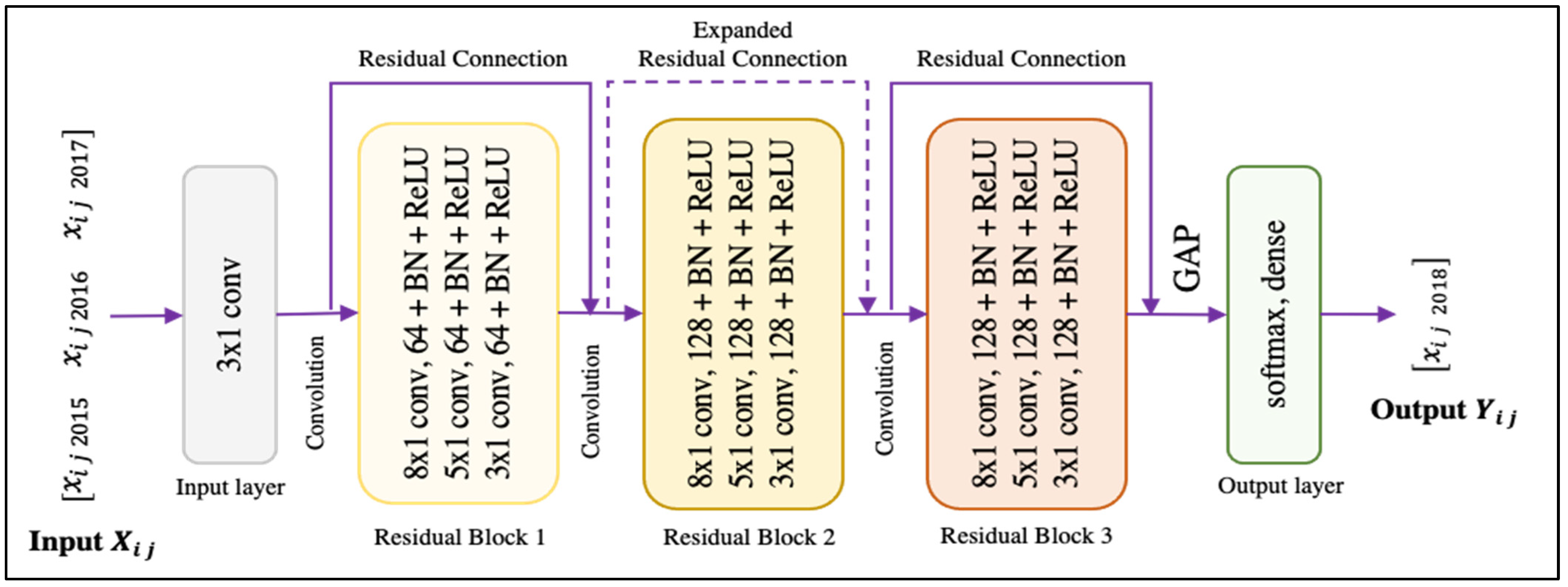
3.1. ResNet Model Setup

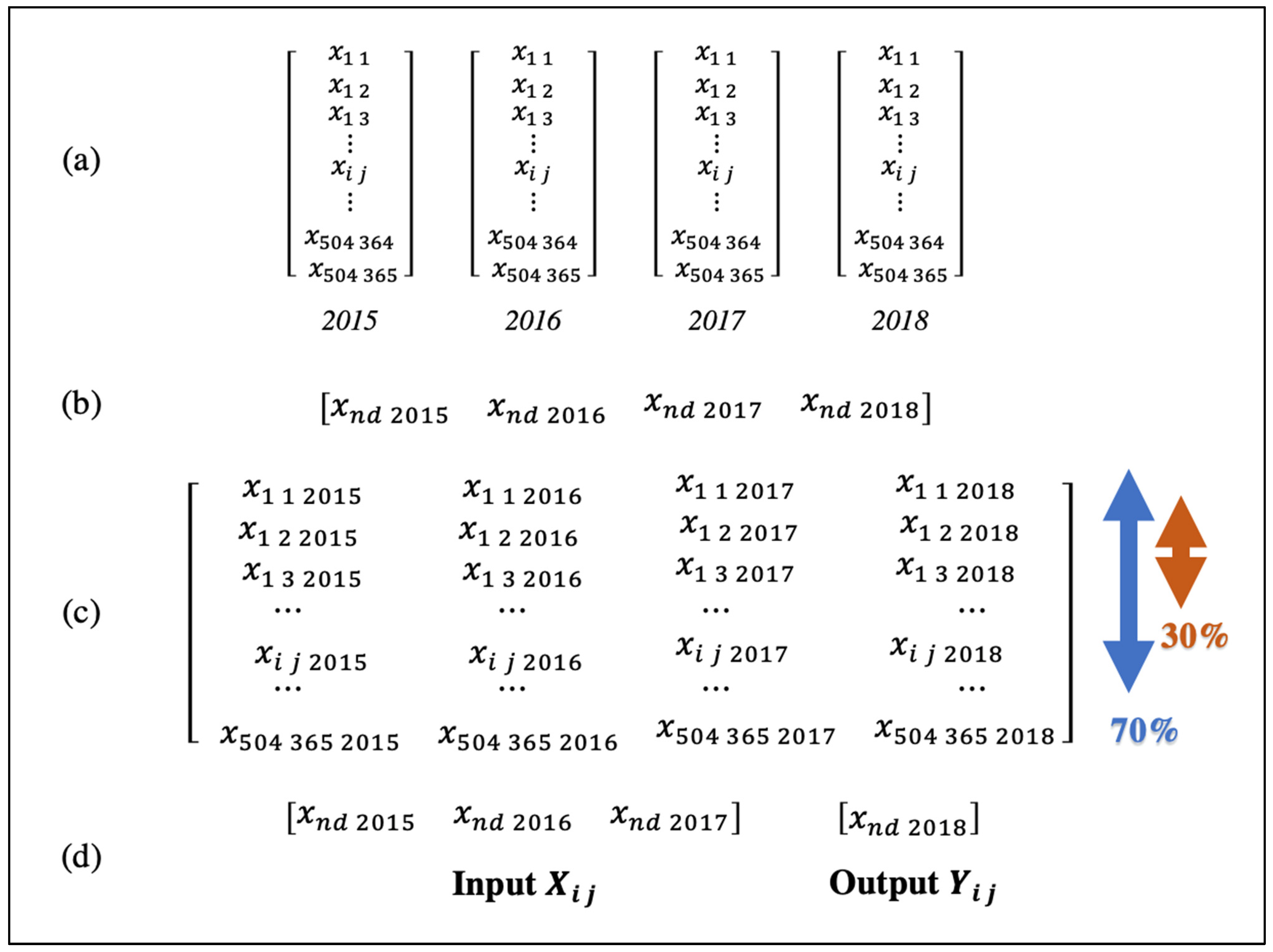
Given the success of ResNet in handling time-series problems, we adopt a ResNet model to predict solar irradiance over the AP. The model, Figure 4, follows the design decisions of earlier studies on time-series analysis [26,47]. The adopted design decisions have also been supported by the empirical results reported in a later study targeting the model sensitivity [48]. Different variants of the ResNet model have been applied to more than 100 datasets. Their study concludes that simpler models of 3 residual blocks surpass much larger models. Therefore, the model applied here has 3 residual blocks, each of which has 3 convolutional layers. The model starts with an input layer where a record will form the input to this layer. In our study, this is a convolutional layer of 3 × 1 where the input has 3 data points. Next, the output of this layer will be fed to the main building blocks of the ResNets model, i.e., the 3 blocks mentioned earlier. Each block has 3 layers of sizes 8 × 1, 5 × 1, and 3 × 1 where each filter has a length of 8, 5, and 3 for the 3 layers of each block, respectively.

The first layer of this block will be applied to the data, which was transferred from the input layer, and it will then be transferred to the second, and then to the third. The input to this block will form the input for the next block, reserving the knowledge and skipping the first block through the residual connection. Each of the convolutional layers is followed by batch normalization and a ReLU activation function. The same process applies to the following 2 blocks, and then this is followed by global average pooling (GAP). GAP is followed by a dense layer that predicts the next time step and reports the expected solar irradiance value in this study. The convolutional layers of the first block have 64 filters, whereas the later layers have 128. Accordingly, the residual connections will expand the output of the first block before adding it to the second block output (see the expanded residual connection in Figure 4). The last dense layer has a SoftMax activation function. The detailed form of the records and the input records at the training and testing phases is declared in the following subsection. We conducted a set of trial-and-error experiments to tune the different model parameters, such as the filters and batch size, etc. The trial-and-error experiments suggested setting the model parameters as shown in

Table 1. ResNet model parameters.

Parameter	Value	Description
Filters	64, 128, 128	Number of output filters of convolutional layers per block
Epochs	1500	Number of iterations for training the model
Batch size	64	Splitting training data into sets of this size
Optimization function	Adam	The method used to minimize the loss while training the model
Learning rate (LR)	0.001	The rate at which the model changes its learning function weights
Reduce on plateau	True	Reduce LR if no further improvements
Reduction factor	0.5	Factor by which LR will be reduced
Patience	50	Number of epochs plateau before reduction

. The model has been implemented on Python using the TensorFlow library through its interface Keras. The training process was held on a device with a 1.2 GHz Dual-Core Intel Core M processor, a memory of 8 GB 1600 MHz DDR3, and an Intel HD Graphics 5300 1536 MB.

To measure the performance of the ResNet model, we recorded different metrics while training it. These metrics are listed in

Table 2. Performance metrics.

Metric	Formula
Mean Squared Error (MSE)	$MSE=\frac{1}{n} {\displaystyle \sum _{i=1}^n}{\left(Y_i-{\widehat{Y}}_i\right)}^2$
Mean Absolute Error (MAE)	$MAE=\frac{1}{n} {\displaystyle \sum _{i=1}^n}(|Y_i-{\widehat{Y}}_i|)$
Coefficient of Determination (R2)	$R^2=1-\frac{{{\displaystyle \sum }}_{i=1}^n{\left(Y_i-{\widehat{Y}}_i\right)}^2}{{{\displaystyle \sum }}_{i=1}^n{\left(Y_i-\overline{Y}\right)}^2}$

, where ${\widehat{Y}}_i$, here, is the predicted value by the model for the test records and $\overline{Y}$ is the mean value of the original observations. In the first and second metrics, the lower value achieved the better. Both metrics report on the expected value of the average error loss when executing the model to predict solar irradiance. The last metric, i.e., the coefficient of determination, represents a measure of how well the values are predicted by the trained model. The higher values, closer to one, are better, whereas lower values reflect worse predictions.

3.2. Dataset

We used average daily solar irradiance data for 4 consecutive years (2015–2018) over the AP (12.5° N–29.5° N, 31.5° E–58.5° E) derived from the RTM model, where MODIS and meteorological data were used as input to the model. Data were then arranged in an 18 × 28 array, where each element of the array represents a 1° × 1° pixel; this procedure resulted in 504 records per day. Accordingly, each year had more than 180,000 data points of 504 locations and 365 days. The data had an average of 181 and a standard deviation ranging from 89 to 94 through the years (further details in

Table 3. Descriptive statistics of solar radiation data considered.

Year	2015	2016	2017	2018
Count	183,960.000000	183,960.000000	183,960.000000	183,960.000000
Mean	184.534849	181.055210	180.143084	181.290188
Std	89.289403	89.154697	92.352037	94.513798
Min	0.088610	0.111343	0.084850	0.089318
Max	444.175800	430.990300	465.336600	440.987000

). In case of missing data, a moving-average window of the values in the most recent 5 days was applied where at least one value should be available. Otherwise, this process was applied repetitively in sequence to fill all missing data. The data were then standardized with a zero mean and a standard deviation of one. Plotting the irradiance values at one location over the considered 4 years, Figure 5, provided a new perspective. The data showed a similar pattern from one year to another. In addition, earlier experiments were conducted to investigate the best record direction across the targeted interval of time as well as its length. The records were initially formed in a horizontal direction meaning that a record had the solar irradiance values of a defined number of consecutive days of the same year. Different trails targeted different lengths. An initial trial built upon a record of 7 consecutive days to predict the 8th day, while another was based on a record of 30 days to predict day 31. However, neither format provided valuable results or valid predictions. Therefore, the input records were formed based on these facts, and a third scenario was tried by the field knowledge as well as the observation obtained from such a figure as Figure 5, where the years have a repetitive pattern. The earlier 3 years’ values form the input part of the record, whereas the value from the 4th year forms the output part (see Figure 6b). In this scenario, although we had such a short-time series of 3 data points across the years per each, it provided us with the required knowledge needed to predict the next year’s solar irradiance value at that specific point of time.

The data generated by the RTM model formed a time series where sequences of daily observations of solar irradiance in the study period (2015–2018) were recorded. We used the ResNets model to find out if the recent states of these time series had a greater impact on the predictable values at next-time steps rather than earlier ones. To examine the effect of spatial resolution on the ResNets model’s efficiency, two scenarios of the solar irradiance data arrays were examined. In the first scenario, all 504 data points in each array were used in the prediction. In the second scenario, the average of each from 4 adjacent locations was used and an array of only 126 data points was formed for the prediction model.

A crucial step during the processing of the time-series data was the formation of an appropriate training dataset for the ResNets model. After formatting the data as shown in Figure 6, a set of 70% of the locations was selected randomly to train the model, while the remaining locations were used to evaluate the model performance. This process was applied for the two scenarios with 504 and 126 data points, respectively. Therefore, 129,210 records were formed for the training phase of the model and 54,750 for its evaluation for the first scenario of 504 sites. In the second scenario of 126 locations, 32,120 records were available for the training and 13,870 for the evaluation phase of the model. The ResNets model was also validated during the training process to ensure that it did not overfit the training data. This way, the ResNets model could be evaluated against the standard RTM model.

4. Results and Discussion

In this section, we present and discuss the experimental results. We start by exploring the data, verifying the RTM model, and diving into the monthly variability of solar irradiance. This is followed by a discussion of the effects of the major events. Finally, the ResNets prediction results are thoroughly analyzed.

4.1. Exploratory Data Analysis

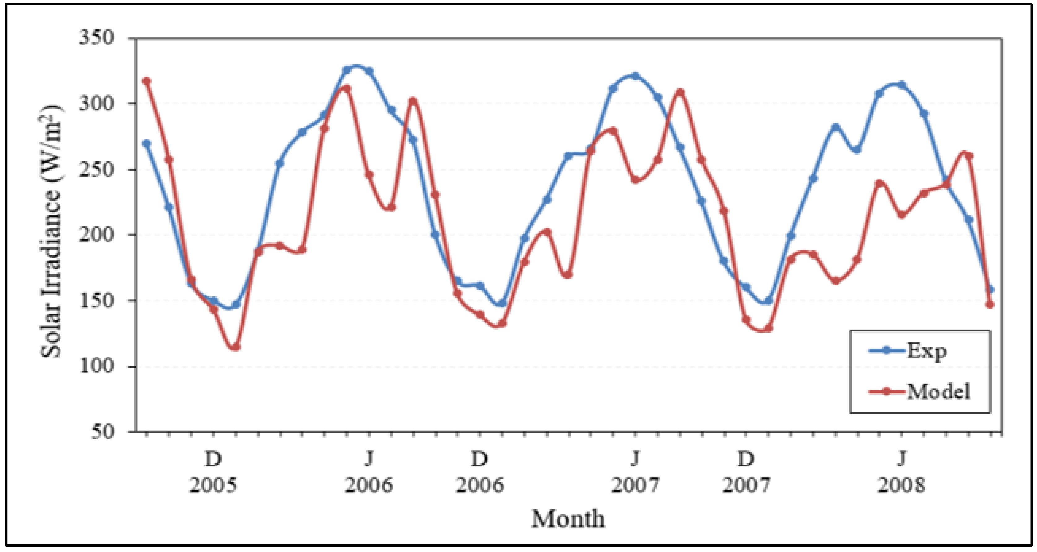
4.1.1. RTM Model Verification

To verify the RTM model output, the results were compared with collected ground-based solar irradiance data. Due to limited ground-data availability, the model was verified with solar ground data from September 2005 to November 2008 only, at the city of Dhahran (26.30° N, 50.146° E) in eastern Saudi Arabia, Figure 7. The data were collected using 250-Watt polycrystalline (FU240-250P) PV panels. Dhahran is located in an arid/semiarid region with high-frequency dust outbreaks and low precipitation (about 80 mm y⁻¹) during the winter and spring seasons [18]. The model showed good agreement with the in-situ measurements except during 2008, Figure 7. It can also be observed that most of the data mismatching takes place during the spring and the summer months. Anti-phase correlation between experimental and simulated solar radiation values during the winter months was also observed. This can be explained by the overestimation of dust loading in the atmosphere by the model during this period.

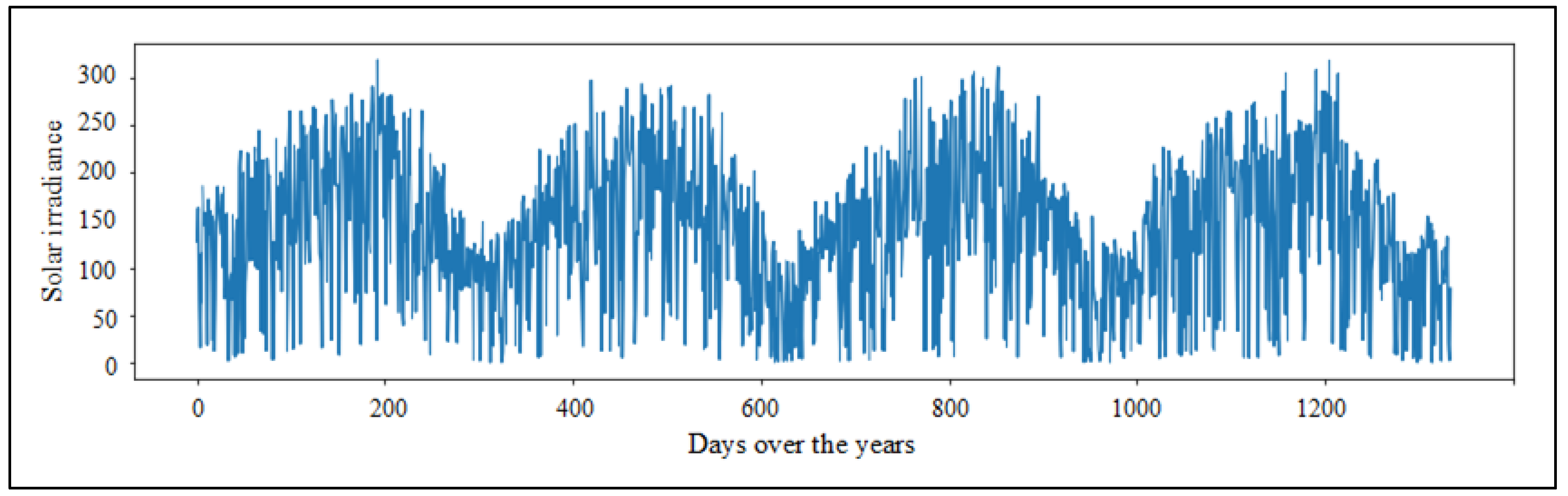
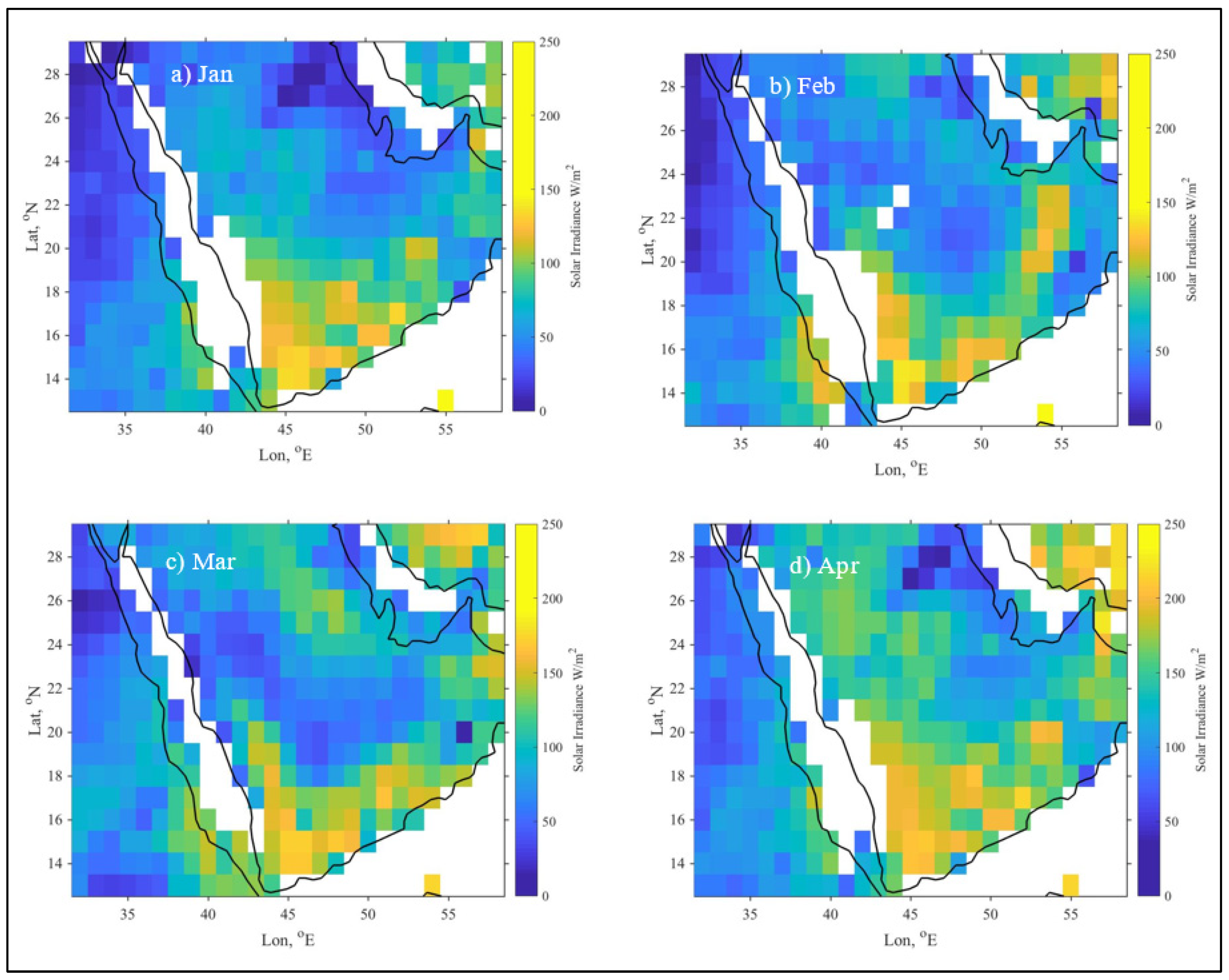
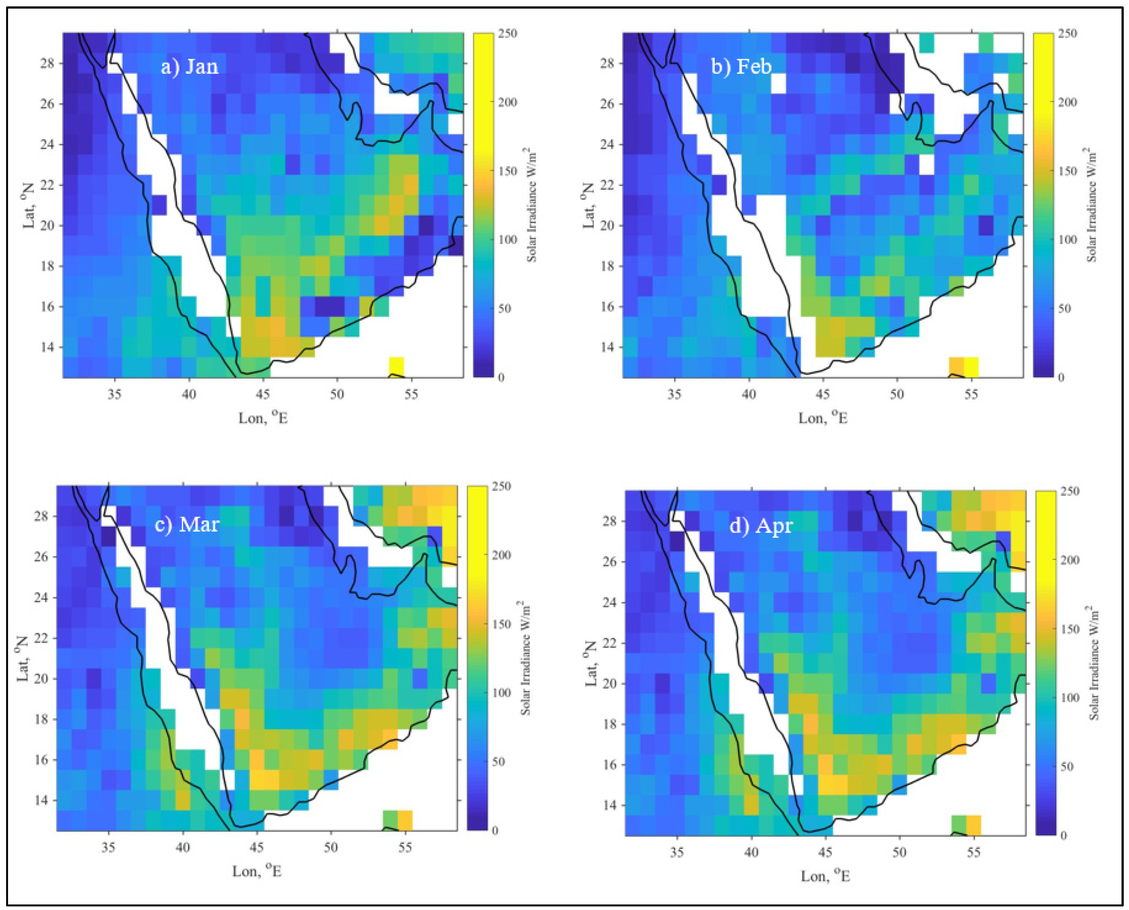
4.1.2. Monthly Variability of Solar Irradiance

Figure 8 and Figure 9 depict the effect of aerosols and dust particles on solar irradiance during January–April of 2016 and 2017 over the AP using the RTM model. These months were selected because of high dust loading and frequent dust outbreaks during the winter and spring seasons over the AP. A monthly variability can be observed with higher solar irradiance values in the southern and southwestern parts of the AP during 2016 (Figure 8). The lower solar irradiance values observed in the eastern parts of the AP may be due to increased aerosol loading that can significantly affect solar irradiance near the Arabian Gulf (AG) and the Sea of Oman (SO) coastlines (~15% less) and central AP (~20% less). Similar trends of dust aerosols loading on solar irradiance can be observed during 2017 (Figure 9).

The southeastern region of the AP, Figure 10, shows the highest solar irradiance during January–April compared to other regions. The figures also show low solar irradiance during March in the eastern region of the AP, which could be attributed to the high frequency of dust events during this time of the year.

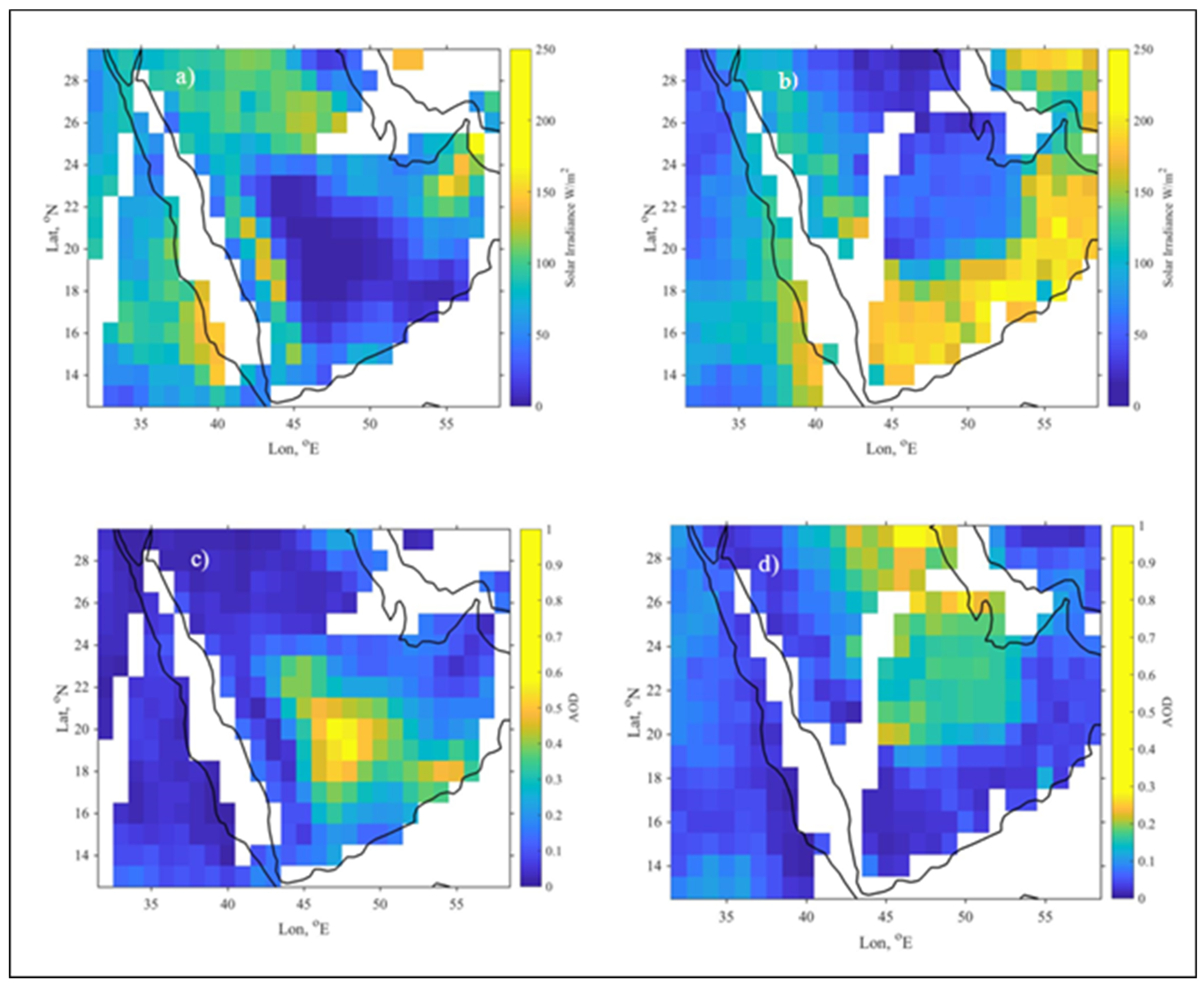
4.2. Effect of Major Dust Events

Major dust outbreaks load the atmosphere with a high concentration of dust particles. Figure 11 displays the effect of 11 March 2009, a day with a major dust storm, on solar irradiance over the AP. The figure clearly illustrates the correlation between high aerosol loading and lower solar irradiance. On 3 March 2009, about 7 days before the storm, high aerosol loading can be observed in the central and southern parts of the AP (Figure 11c). This high aerosol loading resulted in low solar irradiance around the same locations (Figure 11a) where dust loading was high. On 18 March 2009, about 7 days after the storm, lower dust loading can be observed over the same regions of the AP (Figure 11d), with higher solar irradiance (Figure 11b).

Figure 12 shows the effect of dust loading on solar irradiance during the major dust events on 27 March 2012. (Figure 12a,b show the solar irradiance, while Figure 12c,d indicate the corresponding aerosol loading.) On 20 March 2012, 1 week before the major dust event, high aerosol loading was observed over the AP, especially near the Red Sea coast, the AG, and western Iran, with corresponding lower solar radiation levels (Figure 12a,c). On the other hand, on 4 April 2012, 1 week after the storm, low aerosol concentration was observed near the Rub Al Khali desert, with corresponding high solar irradiance.

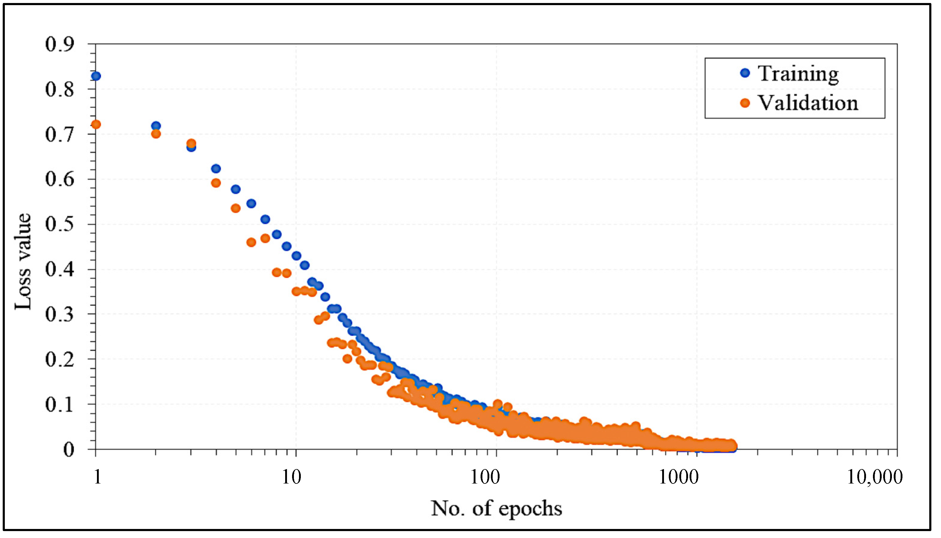
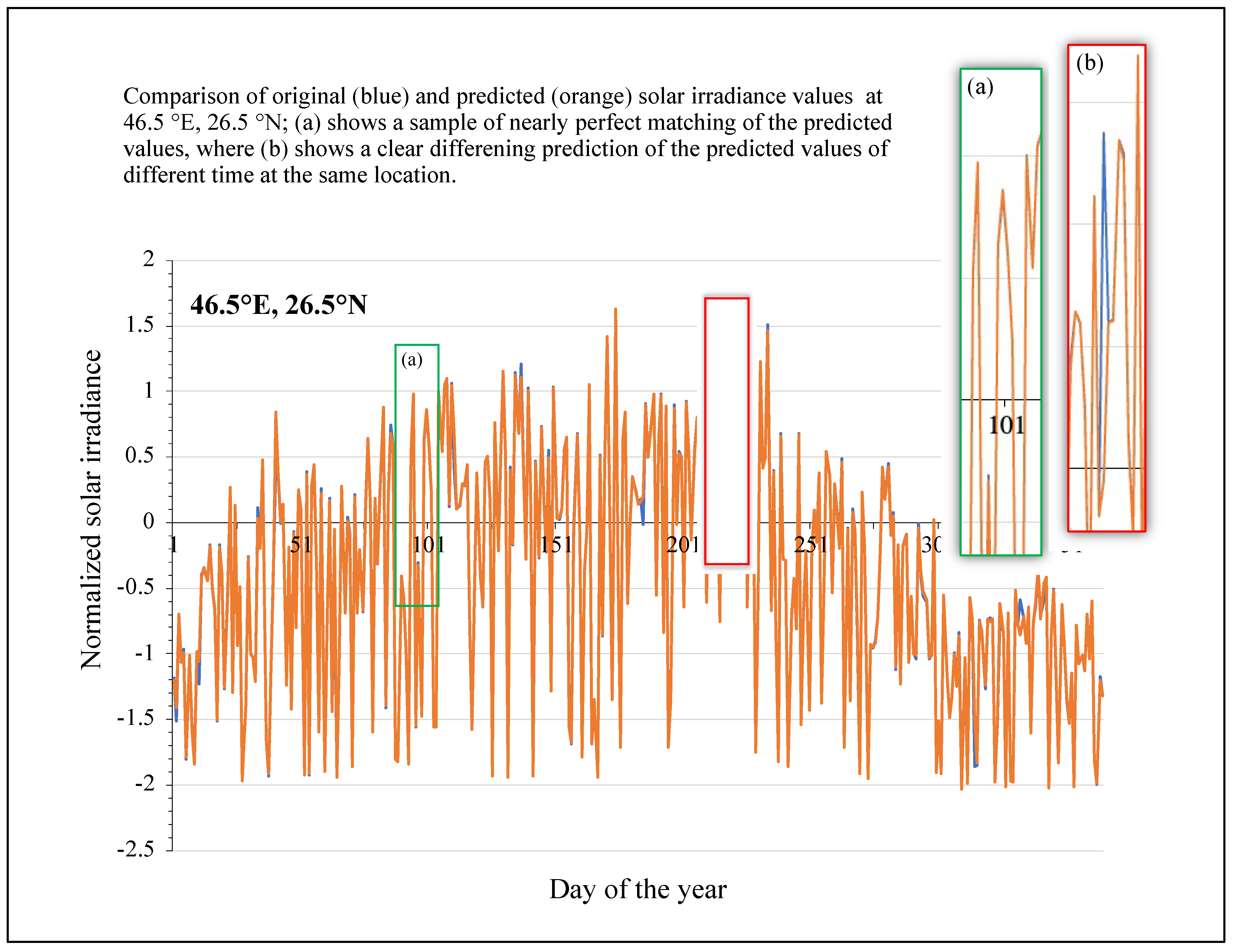
4.3. ResNets Prediction Analysis

The ResNets model was trained for a relatively large number of epochs, 1500, and converged without overfitting the training data (Figure 13).

Table 4. Model performance metrics.

Phase	MAE		MSE		R2
	No of Testing Data Points	No of Training Data Points	No of Testing Data Points	No of Training Data Points	No of Testing Data Points	No of Training Data Points
	126	504	126	504	126	504
Training	0.026148686	0.020791473	0.005544215	0.006416962	0.994715289	0.993957559
Testing	0.026171678	0.020798753	0.005557584	0.006432434	0.993304728	0.992714978
Overall	0.024040448	0.020051688	0.003977843	0.005214457	0.995350867	0.993993272

shows the performance of the model with respect to learning the pattern of data behavior where the generated results by the model were compared to the original data. This comparison shows that the model achieved high accuracy according to the performance metrics presented in Table 2. The model was able to achieve a very low MAE of ~0.02, MSE of ~0.005, and R² of ~0.99. This applies to both the 504 locations scenario and the 126 locations scenario of solar irradiation arrays. There is a slight difference in R² in the range of [0.001–0.002], between the two scenarios. The first scenario required more pre-processing, as we averaged the solar irradiance data for every 4 adjacent locations, where each location is represented by 1° × 1°. Since the results tend to be slightly higher at the second scenario, the first scenario with 504 locations was used while preparing the training dataset of the model, as it encourages less computational time.

It was found that randomizing the input records helped improve the ResNet model’s performance in data prediction. Randomizing the input records is a practice that excludes the existence of any dependence between the input records. This does not affect the values of the records, but it targets the order in which the records are fed to the model during training. Initially, the data were arranged in a matrix where each point is an intersection of one longitude and one latitude. Splitting the matrix into two parts for training and testing without any further adjustment harmed the learning process. The model was able to learn the patterns within the locations of the training part and the near-testing part’s locations only. Predicting the solar irradiance values of the testing part’s locations that were far away from the training part’s locations resulted in a high rate of disturbance in the preliminary experiments. Thus, the data have been assigned differently to the training and testing parts. The matrix values, the locations on the map, were assigned randomly, hence each part had locations that cover the whole map. This process positively affected the learning process and enabled the model to generalize over the considered area.

Another pre-processing step that significantly impacted the model’s performance was the format of the data records. We conducted preliminary experiments where we formatted the records in different lengths and window sizes in order to find the appropriate format that provides the model with the relative knowledge needed to learn the recurrent patterns. Predicting the next day’s solar irradiance value based on the preceding days’ solar irradiance one did not prove informative. However, a recurrent pattern over the years was noticed. Any given day of the considered year will probably have the same solar irradiance value with the same day in the previous years. This observation was utilized to format the data records fed to the model. The data records were built using the solar irradiance values of the same day of every year. Training the model on these records notably affected its performance.

Some design decisions related to the model’s architecture also contributed to the high accuracy of predicting the solar irradiance values. Even though the model was trained for many epochs, 1500, the presence of batch normalization as a regulator technique saved the model from overfitting the training data and enabled an extensive learning process.

A comparison between the original and predicted data at a sample location (Figure 10) is illustrated in Figure 14. The figure shows the accuracy of the ResNet model in predicting the original data over several locations of the AP.

5. Conclusions

The Arabian Peninsula has rich potential for solar energy. Solar photovoltaic (PV) panels could be very important when it comes to harnessing solar energy over the AP. The AP, however, hosts some of the largest deserts in the world, which makes it frequently affected by dust storms that load large amounts of aerosols and dust into the atmosphere. Additionally, the AP hosts the Gulf Council Cooperation (GCC) countries, which are one of the largest oil and natural gas producers in the world. This large petrochemical industry also loads large amounts of anthropogenic aerosols into the atmosphere of the AP. This study focused on the assessment of the aerosol effects on solar irradiance in the AP. It also provided a machine learning tool to predict solar energy over the AP. Data from a moderate resolution imaging spectroradiometer (MODIS) instrument onboard the Terra satellite along with a radiative transfer model and the ResNet machine learning technique were integrated to predict direct solar irradiance on a horizontal surface over the Arabian Peninsula. Solar irradiance data from 2015 to 2017 (100%) and from 2018 (70%) were then used as input to train the ResNet machine learning model in order to predict 2018 (remaining 30%) solar irradiance data. The prediction model achieved high-test scores, indicated by an MAE of ~0.02, MSE of ~0.005, and R² of 0.99 or higher.

The aerosol loading in the atmosphere was found to affect solar irradiance in the eastern region of the AP, especially near the coastlines of the Arabian Gulf and the Sea of Oman (~15%) and central AP (~20%). Low solar irradiance was observed during March 2016 and 2017 in the eastern regions of the AP, which could be attributed to the high frequency of dust events during this time of the year. Compared to other locations in the AP, high solar irradiance was recorded in the southeast regions during winter and spring. The effect of major dust outbreaks blown over the AP during March 2009 and March 2012 was also examined. The results indicated a correlation between high aerosol loading and a decrease in solar irradiance.

References

1. Solangi, K.H.; Islam, M.R.; Saidur, R.; Rahim, N.A.; Fayaz, H. A Review on Global Solar Energy Policy. Renew. Sustain. Energy Rev. 2011, 15, 2149–2163. [Google Scholar] [CrossRef]
2. Hyperwall: Monthly Solar Insolation. Available online: https://svs.gsfc.nasa.gov/cgi-bin/details.cgi?aid=30367 (accessed on 27 October 2021).
3. Moreno, L.E.G. Concentrated Solar Power (CSP) in DESERTEC—Analysis of Technologies to Secure and Affordable Energy Supply. In Proceedings of the 6th IEEE International Conference on Intelligent Data Acquisition and Advanced Computing Systems, Prague, Czech Republic, 15–17 September 2011; Volume 2, pp. 923–926. [Google Scholar]
4. ACWA POWER|Sakaka PV IPP. Available online: https://acwapower.com/en/projects/sakaka-pv-ipp/ (accessed on 10 November 2021).
5. Farahat, A.; Kambezidis, H.D.; Almazroui, M.; Ramadan, E. Solar Potential in Saudi Arabia for Southward-Inclined Flat-Plate Surfaces. Appl. Sci. 2021, 11, 4101. [Google Scholar] [CrossRef]
6. Farahat, A.; Kambezidis, H.D.; Almazroui, M.; Al Otaibi, M. Solar Potential in Saudi Arabia for Inclined Flat-Plate Surfaces of Constant Tilt Tracking the Sun. Appl. Sci. 2021, 11, 7105. [Google Scholar] [CrossRef]
7. Kambezidis, H.D.; Farahat, A.; Almazroui, M.; Ramadan, E. Solar Potential in Saudi Arabia for Flat-Plate Surfaces of Varying Tilt Tracking the Sun. Appl. Sci. 2021, 11, 11564. [Google Scholar] [CrossRef]
8. Kaufman, Y.J.; Tanré, D.; Boucher, O. A Satellite View of Aerosols in the Climate System. Nature 2002, 419, 215–223. [Google Scholar] [CrossRef] [PubMed]
9. Bhattacharya, T.; Chakraborty, A.K.; Pal, K. Effects of Ambient Temperature and Wind Speed on Performance of Monocrystalline Solar Photovoltaic Module in Tripura, India. J. Sol. Energy 2014, 2014, 817078. [Google Scholar] [CrossRef] [Green Version]
10. Siddiqui, R.; Bajpai, U. Deviation in the Performance of Solar Module under Climatic Parameter as Ambient Temperature and Wind Velocity in Composite Climate. Int. J. Renew. Energy Res. (IJRER) 2012, 2, 486–490. [Google Scholar]
11. Sayyah, A.; Horenstein, M.N.; Mazumder, M.K. Energy Yield Loss Caused by Dust Deposition on Photovoltaic Panels. Sol. Energy 2014, 107, 576–604. [Google Scholar] [CrossRef]
12. Vardavas, I.M.; Vardavas, I.; Taylor, F. Radiation and Climate: Atmospheric Energy Budget from Satellite Remote Sensing; Oxford University Press: Oxford, UK, 2011; Volume 138. [Google Scholar]
13. Forster, P.; Ramaswamy, V.; Artaxo, P.; Berntsen, T.; Betts, R.; Fahey, D.W.; Haywood, J.; Lean, J.; Lowe, D.C.; Myhre, G. Changes in Atmospheric Constituents and in Radiative Forcing. Chapter 2. In Climate Change 2007. The Physical Science Basis; 2007; Available online: https://www.ipcc.ch/site/assets/uploads/2018/02/ar4-wg1-chapter2-1.pdf (accessed on 10 November 2021).
14. Behrendt, T.; Kuehnert, J.; Hammer, A.; Lorenz, E.; Betcke, J.; Heinemann, D. Solar Spectral Irradiance Derived from Satellite Data: A Tool to Improve Thin Film PV Performance Estimations? Sol. Energy 2013, 98, 100–110. [Google Scholar] [CrossRef]
15. Sokolik, I.N.; Toon, O.B. Direct Radiative Forcing by Anthropogenic Airborne Mineral Aerosols. Nature 1996, 381, 681–683. [Google Scholar] [CrossRef]
16. Miller, R.L.; Tegen, I. Climate Response to Soil Dust Aerosols. J. Clim. 1998, 11, 3247–3267. [Google Scholar] [CrossRef]
17. Miller, R.L.; Tegen, I.; Perlwitz, J. Surface Radiative Forcing by Soil Dust Aerosols and the Hydrologic Cycle. J. Geophys. Res. Atmos. 2004, 109. [Google Scholar] [CrossRef]
18. Farahat, A. Air Pollution in the Arabian Peninsula (Saudi Arabia, the United Arab Emirates, Kuwait, Qatar, Bahrain, and Oman): Causes, Effects, and Aerosol Categorization. Arab. J. Geosci. 2016, 9, 1–17. [Google Scholar] [CrossRef]
19. Farahat, A.; El-Askary, H.; Adetokunbo, P.; Fuad, A.-T. Analysis of aerosol absorption properties and transport over North Africa and the Middle East using AERONET data. Ann. Geophys. 2016, 34, 1031–1044. [Google Scholar] [CrossRef] [Green Version]
20. Remer, L.A.; Kleidman, R.G.; Levy, R.C.; Kaufman, Y.J.; Tanré, D.; Mattoo, S.; Martins, J.V.; Ichoku, C.; Koren, I.; Yu, H. Global Aerosol Climatology from the MODIS Satellite Sensors. J. Geophys. Res. Atmos. 2008, 113. [Google Scholar] [CrossRef] [Green Version]
21. Alharbi, B.H.; Maghrabi, A.L.; Tapper, N. The March 2009 Dust Event in Saudi Arabia: Precursor and Supportive Environment. Bull. Am. Meteorol. Soc. 2013, 94, 515–528. [Google Scholar] [CrossRef]
22. Mohalfi, S.; Bedi, H.S.; Krishnamurti, T.N.; Cocke, S.D. Impact of Shortwave Radiative Effects of Dust Aerosols on the Summer Season Heat Low over Saudi Arabia. Mon. Weather Rev. 1998, 126, 3153–3168. [Google Scholar] [CrossRef]
23. Saeed, T.M.; Al-Dashti, H.; Spyrou, C. Aerosol’s Optical and Physical Characteristics and Direct Radiative Forcing during a Shamal Dust Storm, a Case Study. Atmos. Chem. Phys. 2014, 14, 3751–3769. [Google Scholar] [CrossRef] [Green Version]
24. Jish Prakash, P.; Stenchikov, G.; Kalenderski, S.; Osipov, S.; Bangalath, H. The Impact of Dust Storms on the Arabian Peninsula and the Red Sea. Atmos. Chem. Phys. 2015, 15, 199–222. [Google Scholar] [CrossRef] [Green Version]
25. Bangalath, H.K.; Stenchikov, G. Role of Dust Direct Radiative Effect on the Tropical Rain Belt over Middle East and North Africa: A High-Resolution AGCM Study. J. Geophys. Res. Atmos. 2015, 120, 4564–4584. [Google Scholar] [CrossRef] [Green Version]
26. Fawaz, H.I.; Forestier, G.; Weber, J.; Idoumghar, L.; Muller, P.-A. Deep Learning for Time Series Classification: A Review. Data Min. Knowl. Discov. 2019, 33, 917–963. [Google Scholar] [CrossRef] [Green Version]
27. Lim, B.; Zohren, S. Time Series Forecasting with Deep Learning: A Survey. arXiv 2020, arXiv:2004.13408. [Google Scholar] [CrossRef] [PubMed]
28. Gueymard, C. SMARTS2: A Simple Model of the Atmospheric Radiative Transfer of Sunshine: Algorithms and Performance Assessment; Florida Solar Energy Center: Cocoa, FL, USA, 1995. [Google Scholar]
29. Mayer, B.; Kylling, A. The LibRadtran Software Package for Radiative Transfer Calculations-Description and Examples of Use. Atmos. Chem. Phys. 2005, 5, 1855–1877. [Google Scholar] [CrossRef] [Green Version]
30. Wu, J.; Zhang, Z.; Ji, Y.; Li, S.; Lin, L. A ResNet with GA-Based Structure Optimization for Robust Time Series Classification. In Proceedings of the 2019 IEEE International Conference on Smart Manufacturing, Industrial & Logistics Engineering (SMILE), Hangzhou, China, 20–21 April 2019; pp. 69–74. [Google Scholar]
31. Alzahrani, A.; Shamsi, P.; Dagli, C.; Ferdowsi, M. Solar Irradiance Forecasting Using Deep Neural Networks. Procedia Comput. Sci. 2017, 114, 304–313. [Google Scholar] [CrossRef]
32. Benali, L.; Notton, G.; Fouilloy, A.; Voyant, C.; Dizene, R. Solar Radiation Forecasting Using Artificial Neural Network and Random Forest Methods: Application to Normal Beam, Horizontal Diffuse and Global Components. Renew. Energy 2019, 132, 871–884. [Google Scholar] [CrossRef]
33. Kylling, A.; Stamnes, K.; Tsay, S.-C. A Reliable and Efficient Two-Stream Algorithm for Spherical Radiative Transfer: Documentation of Accuracy in Realistic Layered Media. J. Atmos. Chem. 1995, 21, 115–150. [Google Scholar] [CrossRef]
34. Hatzianastassiou, N.; Fotiadi, A.; Matsoukas, C.; Pavlakis, K.; Drakakis, E.; Hatzidimitriou, D.; Vardavas, I. Long-Term Global Distribution of Earth’s Shortwave Radiation Budget at the Top of Atmosphere. Atmos. Chem. Phys. 2004, 4, 1217–1235. [Google Scholar] [CrossRef] [Green Version]
35. Hatzianastassiou, N.; Katsoulis, B.; Vardavas, I. Global Distribution of Aerosol Direct Radiative Forcing in the Ultraviolet and Visible Arising under Clear Skies. Tellus B Chem. Phys. Meteorol. 2004, 56, 51–71. [Google Scholar] [CrossRef]
36. Hatzianastassiou, N.; Katsoulis, B.; Vardavas, I. Sensitivity Analysis of Aerosol Direct Radiative Forcing in Ultraviolet—Visible Wavelengths and Consequences for the Heat Budget. Tellus B Chem. Phys. Meteorol. 2004, 56, 368–381. [Google Scholar]
37. Hatzianastassiou, N.; Matsoukas, C.; Drakakis, E.; Stackhouse, P.W., Jr.; Koepke, P.; Fotiadi, A.; Pavlakis, K.G.; Vardavas, I. The Direct Effect of Aerosols on Solar Radiation Based on Satellite Observations, Reanalysis Datasets, and Spectral Aerosol Optical Properties from Global Aerosol Data Set (GADS). Atmos. Chem. Phys. 2007, 7, 2585–2599. [Google Scholar] [CrossRef] [Green Version]
38. NOAA. Land-Based Station Data|National Centers for Environmental Information (NCEI) Formerly Known as National Climatic Data Center (NCDC)—Google. Available online: https://www.google.com/search?q=.+NOAA%2C+Land-Based+Station+Data+%7C+National+Centers+for+Environmental+Information+%28NCEI%29+Formerly+Known+as+National+Climatic+Data+Center+%28NCDC%29&ei=VnF5YcufIM3bgwfs1afABQ&ved=0ahUKEwjLopqN9erzAhXN7eAKHezqCVgQ4dUDCA4&uact=5&oq=.+NOAA%2C+Land-Based+Station+Data+%7C+National+Centers+for+Environmental+Information+%28NCEI%29+Formerly+Known+as+National+Climatic+Data+Center+%28NCDC%29&gs_lcp=Cgdnd3Mtd2l6EAMyBwgAEEcQsAMyBwgAEEcQsAMyBwgAEEcQsAMyBwgAEEcQsAMyBwgAEEcQsAMyBwgAEEcQsAMyBwgAEEcQsAMyBwgAEEcQsANKBAhBGABQhqECWIahAmCrrwJoAHAFeACAAQCIAQCSAQCYAQCgAQHIAQjAAQE&sclient=gws-wiz (accessed on 27 October 2021).
39. Goodfellow, I.; Bengio, Y.; Courville, A. Deep Learning; MIT Press: Cambridge, UK, 2016; Volume 1. [Google Scholar]
40. Chu, D.A.; Kaufman, Y.J.; Ichoku, C.; Remer, L.A.; Tanré, D.; Holben, B.N. Validation of MODIS Aerosol Optical Depth Retrieval over Land. Geophys. Res. Lett. 2002, 29, MOD2-1. [Google Scholar] [CrossRef] [Green Version]
41. Remer, L.A.; Kaufman, Y.J.; Tanré, D.; Mattoo, S.; Chu, D.A.; Martins, J.V.; Li, R.-R.; Ichoku, C.; Levy, R.C.; Kleidman, R.G. The MODIS Aerosol Algorithm, Products, and Validation. J. Atmos. Sci. 2005, 62, 947–973. [Google Scholar] [CrossRef] [Green Version]
42. Roesch, A.; Schaaf, C.; Gao, F. Use of Moderate-Resolution Imaging Spectroradiometer Bidirectional Reflectance Distribution Function Products to Enhance Simulated Surface Albedos. J. Geophys. Res. Atmos. 2004, 109. [Google Scholar] [CrossRef] [Green Version]
43. Schaaf, C.B.; Gao, F.; Strahler, A.H.; Lucht, W.; Li, X.; Tsang, T.; Strugnell, N.C.; Zhang, X.; Jin, Y.; Muller, J.-P. First Operational BRDF, Albedo Nadir Reflectance Products from MODIS. Remote Sens. Environ. 2002, 83, 135–148. [Google Scholar] [CrossRef] [Green Version]
44. Levy, R.C.; Remer, L.A.; Kleidman, R.G.; Mattoo, S.; Ichoku, C.; Kahn, R.; Eck, T.F. Global Evaluation of the Collection 5 MODIS Dark-Target Aerosol Products over Land. Atmos. Chem. Phys. 2010, 10, 10399–10420. [Google Scholar] [CrossRef] [Green Version]
45. Hsu, N.C.; Tsay, S.-C.; King, M.D.; Herman, J.R. Deep Blue Retrievals of Asian Aerosol Properties during ACE-Asia. IEEE Trans. Geosci. Remote Sens. 2006, 44, 3180–3195. [Google Scholar] [CrossRef]
46. Levy, R.C.; Mattoo, S.; Munchak, L.A.; Remer, L.A.; Sayer, A.M.; Patadia, F.; Hsu, N.C. The Collection 6 MODIS Aerosol Products over Land and Ocean. Atmos. Meas. Tech. 2013, 6, 2989–3034. [Google Scholar] [CrossRef] [Green Version]
47. Wang, Z.; Yan, W.; Oates, T. Time Series Classification from Scratch with Deep Neural Networks: A Strong Baseline. In Proceedings of the 2017 International Joint Conference on Neural Networks (IJCNN), Anchorage, AK, USA, 14–19 May 2017; pp. 1578–1585. [Google Scholar]
48. Alwadei, S.; Ahmed, M. On the Sensitivity of Residual Networks for Time Series Classification. In Proceedings of the 2021 1st International Conference on Artificial Intelligence and Data Analytics (CAIDA), Riyadh, Saudi Arabia, 6–7 April 2021; pp. 234–239. [Google Scholar]
Figure 1. Map of the Arabian Peninsula.
Applsci 12 00717 g001
Figure 2. ResNet example: (a) A typical convolution layer, (b) example of a Residual Block [26,39].
Applsci 12 00717 g002
Figure 3. Schematic diagram of the model structure.
Applsci 12 00717 g003
Figure 4. The ResNets model architecture.
Applsci 12 00717 g004
Figure 5. Visualization of solar irradiance values of a location sample of the years 2016–2018.
Applsci 12 00717 g005
Figure 6. Schematic diagram of the application of the solar radiation data format for the ResNet model from 504 locations in the period 2015–2018. (a) Original time series of the 504 locations resulting in 183,960 data points per year. (b) Proposed data format, where n is the location number and d is the day of the year. (c) The final format of the data, where 70% of n locations were picked randomly for training the model and the remaining 30% of the locations for its evaluation. (d) Input and output time series.
Applsci 12 00717 g006
Figure 7. Model verification using experimental solar irradiance data collected in Dhahran (26.307° N, 50.146° E), Saudi Arabia during September 2005–November 2008.
Applsci 12 00717 g007
Figure 8. Intra-annual direct solar irradiance over AP during (ad) January–April 2016, respectively.
Applsci 12 00717 g008
Figure 9. Intra-annual direct solar irradiance over AP during (ad) January–April 2017, respectively.
Applsci 12 00717 g009
Figure 10. Locations with the highest solar irradiance in the Arabian Peninsula are highlighted in yellow. Points a–f represent locations used to check the efficiency of the machine learning ResNet model.
Applsci 12 00717 g010
Figure 11. Effect of 11 March 2009, a major dust event, on solar irradiance over the AP on (a) 3 March 2009, (b) 18 March 2009; and on AOD over the AP for (c) 3 March 2009, and (d) 18 March 2009.
Applsci 12 00717 g011
Figure 12. Effect of a major dust event, on solar irradiance over the AP on (a) 20 March 2012, (b) 4 April 2012; and on AOD for (c) 20 March 2012, and (d) 4 April 2012.
Applsci 12 00717 g012
Figure 13. Model convergence.
Applsci 12 00717 g013
Figure 14. Comparison of original (blue) and predicted (orange) at (a) 47.5° E, 20.5° N; (b) 50.5° E, 22.5° N.
Applsci 12 00717 g014