Scale Effects on the Calculation of Ecosystem Service Values: A Comparison among Results from Different LULC Datasets

Featured Application

This study investigated the scale effects of ESV from land use/land cover data which is not given enough attention. In addition, the results suggested that ESV values calculated from different datasets with different spatial resolution have significant difference which is very meaningful for future ESV value evaluations.

Abstract

Land use/land cover (LULC) has an important impact on the ecological environment and is crucial for calculating ecosystem service values (ESVs). However, whether and to what extent the ESVs vary when calculated by LULC product data at different spatial scales remain unclear. Data from two LULC products were used in this study, and two datasets with different spatial scales were obtained by resampling. Then, the ESVs were calculated by the equivalent factor method. Finally, the impacts of LULC on ESVs at different scales were studied, revealing the following: (1) The ESVs calculated by LULC products and by the same products at different scales are different. (2) The difference in the ESVs calculated by the two LULC datasets is approximately 28%, and the difference tends to decrease with increasing scale. (3) With an increase in the LULC scale, the overall change trend of ESVs also increases, and the increasing trend gradually moderates. In addition, the ESVs and LULC scale conform to a logarithmic relationship, and the coefficient of determination (R²) is greater than 0.7. These results have important reference value for obtaining reliable ESVs.

1. Introduction

Ecosystem services refers to the direct or indirect production of life support products and services through the structure, process and function of ecosystem [1]. Ecosystem services are critical to human health and survival as well as regional and global ecological security [2,3], and are the frontier and hotspot of ecology and geography research [4]. Ecological systems are crucial not only because they can directly provide all kinds of raw materials and products necessary for human survival but also because they perform purification functions that play significant roles in regulating climate, reducing pollution, conserving water and biodiversity, providing disaster relief, and fixing soil, windbreaks and sand, etc.; all of these functions contribute to human survival, and ecosystem products and services are collectively referred to as ecosystem services [5]. Accordingly, ecosystem services are key to our understanding of the medium- and long-term impacts of changes in biodiversity, climate, land transformation, stratospheric ozone, water and nitrogen on humans [6]. Diminishing ecosystem services have been regarded as an important ecological problem in the 21st century [7]. Hence, with the rapid development of remote sensing technology, increasing amounts of remote sensing data have been applied to the study of ecosystems [7,8,9,10,11].

Changes in land use/land cover (LULC) have considerable effects on the energy budget of the Earth and the biogeochemical cycle, thereby affecting surface properties and ecosystem services [12,13]. A variety of studies on biodiversity [14], the soil carbon cycle [15], water regulation [16], soil regulation [17], atmospheric regulation [18], carbon sequestration [19] and entertainment services [20] have reported relationships between LULC and ecosystem service values (ESVs). Furthermore, research has verified that the variations in LULC can be regarded as a proxy for ecosystems, and LULC variations can be used to calculate the trends of ESVs and ascertain the safety of ecosystems. Consequently, LULC datasets have been used to calculate the ESVs of different regions.

ESVs calculations, which have been deemed the fundamental basis for ecological asset accounting since 1997, facilitate the spatial recognition of ecosystems and manage their sustainability [21]. Currently, two major methods are employed to calculate ESVs: the functional value evaluation method and the equivalent factor method [22]. The functional value evaluation method is based on a series of ecological functions used to evaluate several key service functions and is very complicated [23]. Therefore, this method is more suitable for use at small scales [24]. However, this method is tremendously expensive, and researchers usually lack the background of the research region needed to customize the parameters for these functions, resulting in considerable uncertainty [25]. In contrast, the equivalent factor method establishes the relationships between agricultural products and ESVs based on benefit transfer theory and takes LULC as a quantifiable proxy to indirectly obtain ESVs [26,27]. This method was first proposed by Costanza, et al. [28] for the global scale and was later regarded as unsuitable in China. More recently, Xie, et al. [29] proposed an equivalent factor method for calculating ESVs in China based on surveys that places ecosystem and service functions into categories based on LULC datasets. The values of crops per unit area (1 hm²) of farmland in China were used as references to obtain the equivalent values based on the meta-analysis method. This method has been proven to be suitable in China [30]. Since the equivalent factor method has been shown to be more capable of calculating ESVs at large scales than the functional value evaluation method, this technique has been applied in many studies, for example, at the global scales [28] and in South Africa [31], Nigeria [32], Ethiopia [33] and the Qinghai-Tibet Plateau (QTP) in China [34].

Although the equivalent factor method is relatively popular, this approach relies on LULC to calculate ESVs, and different (even the same) LULC products have different spatial scales. Nevertheless, while the different spatial scales of different LULC products may affect ESVs calculations, the impacts of variations in the spatial scale have not been clearly investigated. To address the problem of different scales among different LULC products, we used data from two LULC products and obtained two sets of data at different spatial scales by resampling. We then calculated the ESVs by implementing the equivalent factor method to obtain the differences caused by different LULC products.

In this study, data from two LULC products in 2010 were used. Each product consisted of 13 spatial scales ranging from 300 m to 3900 m, and the LULC data had a scale difference of 300 m between the two products. Taking the QTP as the study area, the ESVs were calculated by the equivalent factor method. The main research objectives were as follows: (1) to analyze the differences in different LULC products with changes in the spatial scale; (2) to calculate the ESVs from the LULC data of different products and from the same product at different spatial scales; and (3) to study the change trend of the ESVs of LULC at different scales.

2. Study Area and Dataset

2.1. Study Area

The QTP extends from the southern margin of the Himalayas in the south to the northern margin of the Kunlun, Altun and Qilian Mountains in the north, the Pamir Plateau and the Karakoram Mountains in the west, and the western segment of the Qinling Mountains and the Loess Plateau to the east and northeast. The plateau is approximately 2800 km long from east to west and 300~1500 km wide from north to south. The Chinese portion of the QTP extends from 26°00′12″ N to 39°46′50″ N and from 73°18′52″ E to 104°46′59″ E (Figure 1a). The QTP is the largest plateau in China and the highest plateau in the world; hence, it is commonly known as the “Roof of the World” and the “Third Pole”. Moreover, the QTP is the highest and youngest natural geographical unit in the world with a close combination of horizontal and vertical zonality, with an elevation generally between 3000 and 5000 m above sea level and an average elevation exceeding 4000 m (Figure 1b). The QTP is the source of many great rivers that run through East, Southeast and South Asia, and the average annual temperature in its hinterland is below 0 °C, with the average temperature in the warmest month being lower than 10 °C in large areas. The plateau promotes tremendous species and ecosystem diversity and provides a variety of important ecosystem services, such as water, timber, rangeland and recreational opportunities, for more than 1.5 billion people. However, the region is extremely vulnerable to climate change and human activities [34], which have led to significant LULC, including lake shrinkage and expansion, permafrost loss, grassland degradation, desertification, deforestation and urbanization.

2.2. Dataset

The first kind of LULC data adopted in this study come from the Climate Change Initiative Land Cover (CCI LC) dataset of the European Space Agency (ESA, Paris, France); this product offers LULC data with some of the highest temporal and spatial resolutions available at present. These data are acquired by using a multiyear and multisensory strategy to maximize the consistency of the product with a spatial resolution of 300 m (http://maps.elie.ucl.ac.be/CCI/viewer/index.php, accessed on 20 December 2021). The other kind of LULC data are from the Resources and Environmental Science and Data Center (RES, Beijing, China, http://www.resdc.cn/, accessed on 20 December 2021), whose data are produced based on Landsat TM/ETM remote sensing images of each period as the main data source [35] and generated through manual visual interpretation with a spatial resolution of 30 m. The two LULC datasets selected in this paper both cover the year 2010.

3. Methods

3.1. Land Use Change

The change amplitude of a certain LULC type in the study area is usually expressed and measured by a single land use dynamic degree and is of great significance to analyzing regional differences in LULC change [33,36]:

$$\mathrm{K}=\left|\frac{U_b-U_a}{U_a}\right|\times 100\%$$

(1)

where K is the dynamic degree of a certain land type in the study area, U_b is the area of a land type in the study area at a certain scale, and U_a is the area of the same land type in the study area at another scale.

3.2. Calculation of ESVs

In this study, the equivalent factor method of Xie, Zhang, Zhen and Zhang [22] was used to calculate the ESVs in the study area. This method defines a standard equivalent factor as the economic value of the annual natural grain yield of farmland with a national average yield of 1 hm². A standard equivalent factor of ESVs can refer to the net profit of food production per unit area of farmland ecosystem. The formula for calculating the grain yield per unit of farmland ecosystem is as follows:

$$W=P_1\times W_1+P_2\times W_2+P_3\times W_3$$

(2)

where $W$ is the ESVs of a standard equivalent factor (yuan/hm²); $P_1$, $P_2$ and $P_3$ are the proportions of wheat, maize and rice, respectively, among the total area of these three crops in 2010 (%); and $W_1$, $W_2$ and $W_3$ are the net profits per unit area (yuan/hm²) of wheat, corn and rice in 2010, respectively. The agricultural data were obtained from the 2011 China Statistical Yearbook and the 2011 National Agricultural Product Cost and Income Data Compilation. According to the data and Formula (1), W was calculated as 3406.5 yuan/hm².

The formula for calculating the ESVs is as follows:

$${\mathrm{VC}}_{fi}={\mathrm{EC}}_{fi}\times E_a$$

(3)

$$\mathrm{ESV}s={{\displaystyle \sum }}_{i=1}^n\left(A_i\times {{\displaystyle \sum }}_{f=1}^k{\mathrm{VC}}_{fi}\right)$$

(4)

where $\mathrm{ESV}s$ denotes the ecosystem service values of the study area, $E_a$ is a standard equivalent ESVs, ${\mathrm{VC}}_{fi}$ is the ESVs coefficient of the $i$-th LULC type, $E{C}_{fi}$ is the ESVs equivalent of the $f$-th ecosystem service of the $i$-th LULC type, and A_i is the area of the $i$-th LULC type. The ecosystem service function of construction land is not significant, and its ESVs was set as 0 in this study, so construction land was not included in the calculation of ESVs.

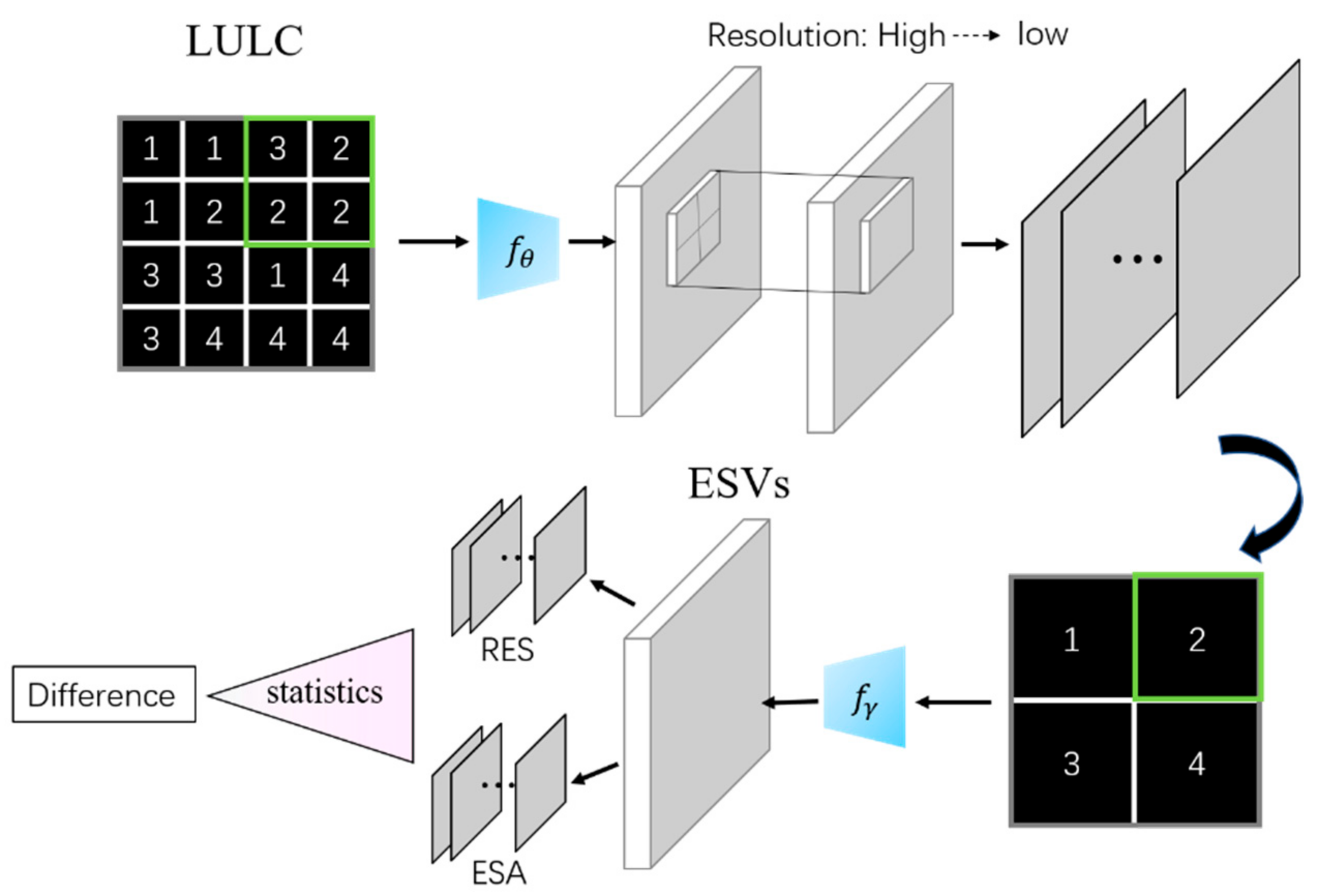
3.3. Influence of LULC on ESVs at Different Scales

To analyse the impact of LULC on ESVs at different scales, a series of LULC data at different scales should be obtained first. The basic LULC data used in this paper were derived from the ESA and RES datasets. The two datasets were scaled up 12 times each. The 300 m ESA LULC data were upscaled at an interval of 300 m, yielding ESA LULC data on 13 different scales. However, since the spatial scale of the RES LULC data is only 30 m, to maintain consistency with the 13 ESA scales, the 30 m data were first upscaled to 300 m and then scaled an additional 12 times. After obtaining the LULC data on different scales for both products, Formulas (3) and (4) were used to calculate the ESVs, and finally, the differences in the ESVs were obtained. The overall operation is depicted in Figure 2, where $f_{\theta }$ denotes the ESVs calculation method. For the selection of pixel values after upscaling the data, the mode method is adopted in this paper, and the formula is as follows:

$$f_{\theta }=L+\frac{f_b}{f_a+f_b}·i$$

(5)

where $L$ is the lower limit of the group in which the mode is located, $f_a$ is the frequency adjacent to the lower limit of the mode array, $f_b$ is the frequency adjacent to the upper limit of the mode array, and $i$ is the group distance.

4. Results

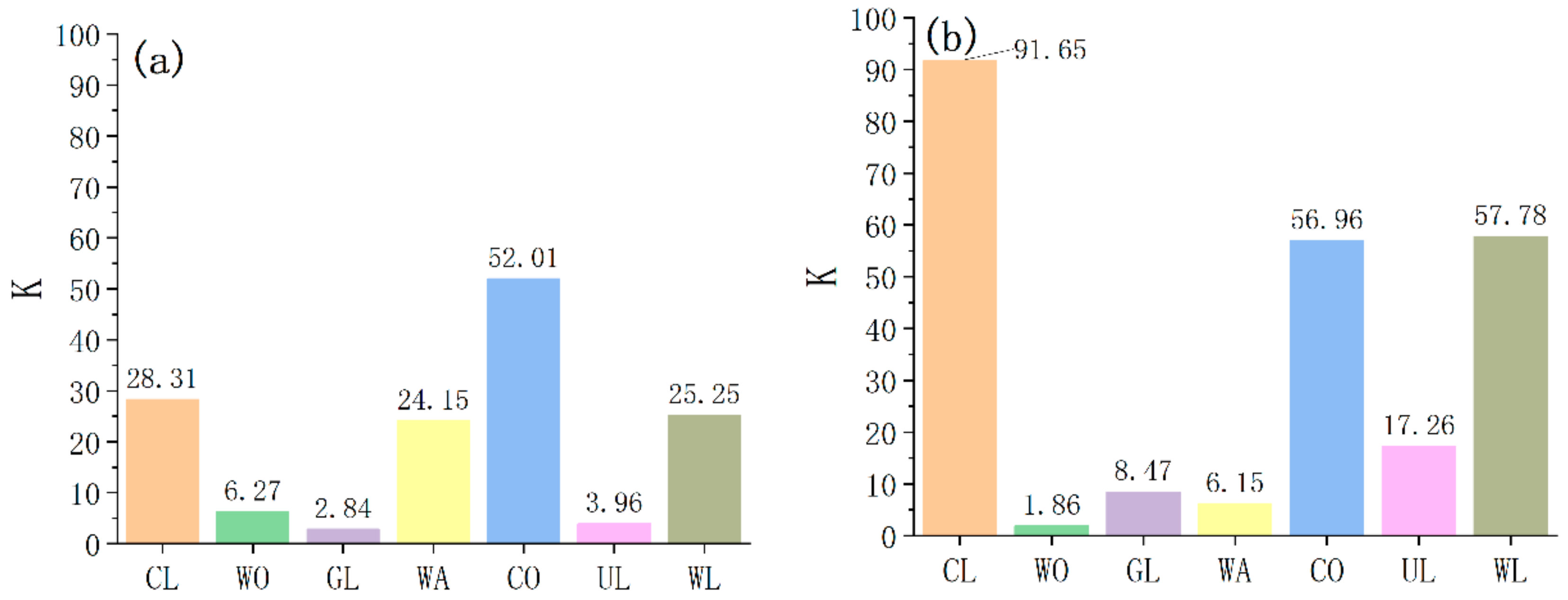
4.1. Changes in Different LULC Products

To analyse how the areas of different LULC types change with the scale, the area of each LULC type at each scale is calculated in this paper, yielding numerous area change trend charts (Figure 3). As shown in Figure 3, there are differences between the ESA and RES LULC data: the area of grassland (GL) exhibits the largest difference, with an average difference of 534,207.99 km², while that of construction land (CO) has the smallest difference, with an average difference of 936.13 km². With increasing scale, between the two LULC products, the differences in the area of woodland (WO), water bodies (WA), CO and wetland (WL) tend to decrease and the difference value decreases by 24,425.55 km², 4690.35 km², 97 km² and 3065.85 km², respectively, while those of GL and unused land (UL) tend to increase, and that of cropland (CL) first increases and then decreases, and the difference increased by 21,055.50 km² and 110,847.60 km², respectively. Moreover, the LULC types that display change trends of similar appearance with increasing scale include CL, WO, WA, CO and WL; among them, CL has an upward trend, while the others all have a downward trend. In addition, from the perspective of stability, as the scale changes, ESA CL and RES WA change the most, indicating that these two LULC types are not stable, whereas the change trends of the other LULC types are relatively stable. Figure 3h shows the overall area change trend of both datasets, revealing little variation in the overall area. With an increase in the scale, the overall land use area also increases, increasing by 1644.75 km²; however, this accounts for only 0.06% of the total area, indicating that an increase in the scale has little influence on the overall area.

The degree of LULC change was further analyzed. For this purpose, the dynamic degree of LULC K was calculated (Figure 4). The LULC data at spatial scales of 300 m and 3900 m were used. For RES, the change amplitude of CO is the largest with a K value of 52.01, while the change amplitude of GL is the smallest with a K value of 2.84. For ESA, CL has the largest change with a K value of 91.65, and WO has the smallest change with a K value of 1.86. In general, the scale appears to have a considerable influence on the areas of GL, CO and CL.

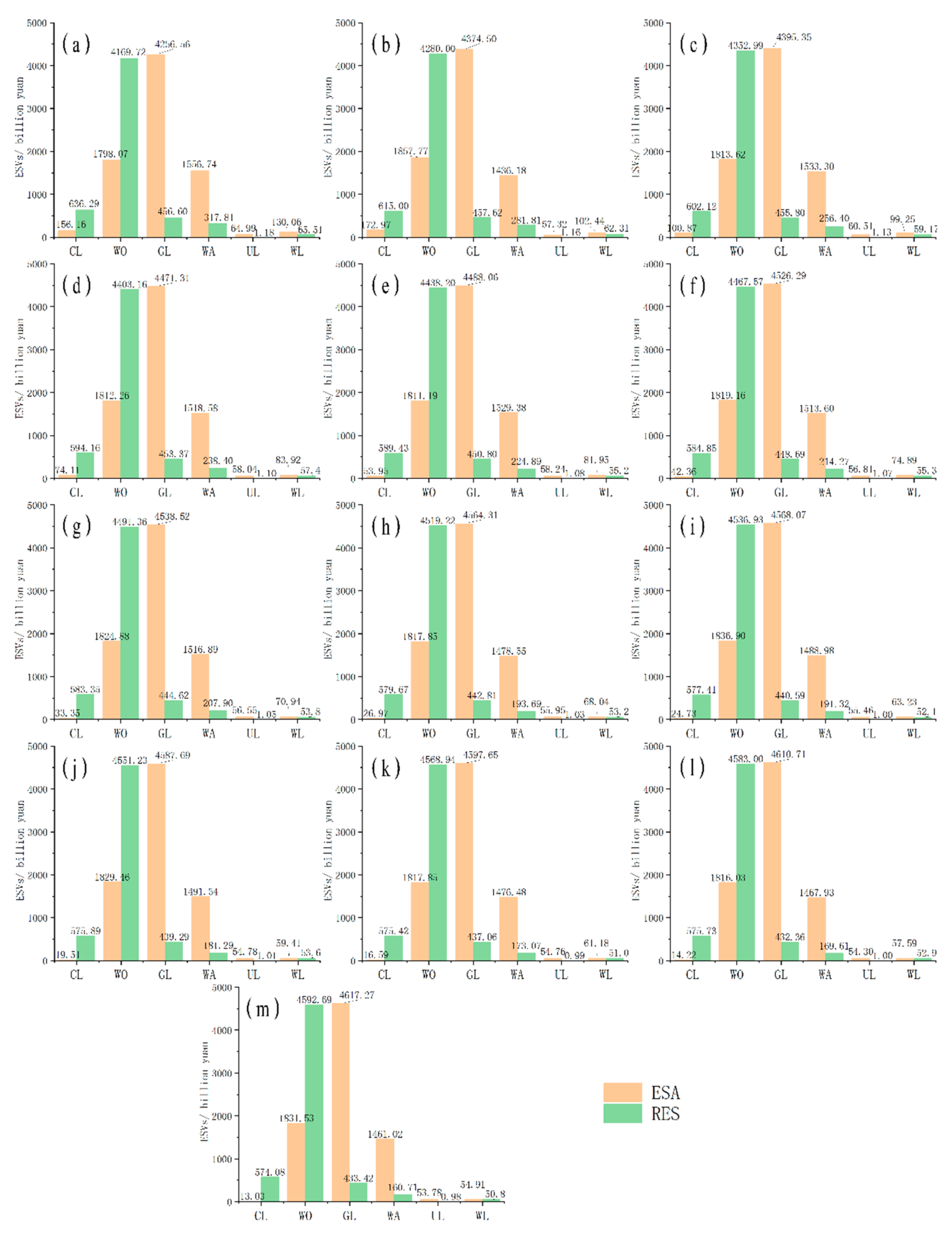
4.2. ESVs of Different LULC Types

The ESVs were further calculated for all LULC types at different scales (Figure 5). The ESVs of RES and ESA are different for different LULC types at different scales, and the ESVs rankings corresponding to the LULC types differ between the two LULC products. The ESVs ranking of ESA for all LULC types is GL > WO > WA > CL > WL > UL; the ESVs of GL can reach more than 4200 billion yuan, representing the maximum, while that of UL is less than 70 billion yuan, signifying the lowest ESVs. For RES, the ESVs ranking for all LULC types is WO > CL > GL > WA > WL > UL; the ESVs of WO exceeds 4100 billion yuan, while that of UL is less than 2 billion yuan. In addition, the overall ESVs calculated by different LULC product data also differ (

Table 1. Overall ESVs of ESA and RES at different scales and their differences.

Scale (m)	ESVs (Billion Yuan)		Difference (%)
	ESA	RES
300	7962.59	5647.11	29.08
600	8001.19	5697.90	28.79
900	8002.90	5727.62	28.43
1200	8018.20	5747.61	28.32
1500	8022.77	5759.58	28.21
1800	8033.11	5771.83	28.15
2100	8041.12	5782.11	28.09
2400	8011.67	5789.69	27.73
2700	8037.35	5799.36	27.84
3000	8042.39	5802.37	27.85
3300	8024.51	5806.49	27.64
3600	8020.77	5814.64	27.51
3900	8031.54	5812.77	27.63

). The ESVs calculated by ESA is about 8000 billion yuan, and the ESVs calculated by RES is about 5700 billion yuan. Compared with the difference among the ESVs of ESA, the difference among the ESVs of RES is approximately 28%, and this difference tends to decrease with increasing scale. In general, the ESVs vary when calculated by the LULC data of different products or even by the LULC data of the same product at different scales.

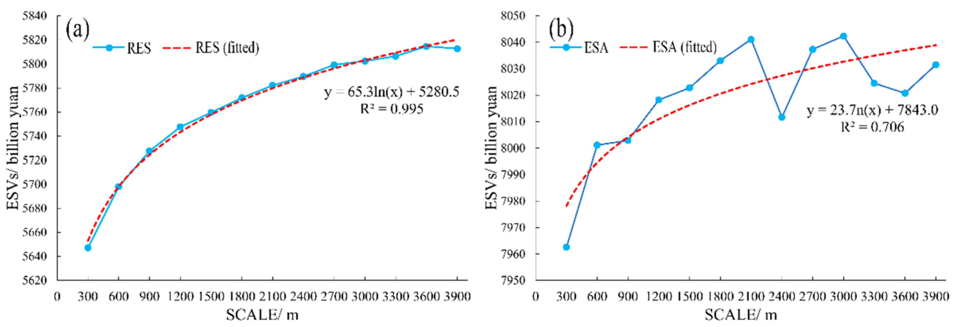
4.3. Effects of the Spatial Scale

LULC types at different scales were used to calculate the ESVs of corresponding scales. To analyze the influence of scale on ESVs, we calculate the change trend of the ESVs with increasing scale (Figure 6). As shown in Figure 6, with an increase in the LULC scale, the overall change trend of ESVs also increases. Compared with that of ESA, the change trend of RES is more stable and exhibits less fluctuation in the trend, and the ESVs consistently agree with the increasing scale. Furthermore, as the LULC scale of RES and ESA increases, the rate of increase in the ESVs trend gradually slows, so we employed a logarithmic function to fit the scale and ESVs. The fitting results indicate that the correlations of determination (R²) of the data from the two products are both greater than 0.7, with that of RES reaching as high as 0.995. These findings confirm that the relationship between the ESVs and scale is logarithmic.

5. Discussion

5.1. Effects of the Spatial Scale

LULC changes can greatly change the Earth’s energy balance and biogeochemical cycle, thereby affecting the surface characteristics and provision of ecosystem services. Therefore, LULC data are often used to calculate ESVs. However, the calculation of ESVs by LULC depends on the spatial scale of LULC.

Studies have revealed differences between different LULC datasets (e.g., RES and ESA) that may be caused by different sensors or interpretation methods [37]. With changes in scale, the areas of different LULC types are always changing, and the overall area increases. Scale has substantial impacts on the areas of GL, CO and CL. Since the mode method was adopted in this paper to upscale the data, the LULC types in different spaces continue to converge to the mode values, which is similar to the results of existing spatial scale studies [38]. Overall, the ESVs calculated by different LULC product data also differ. Compared with the ESVs calculated for the ESA LULC data, those calculated for the RES data differ by approximately 28%, which is attributable to the difference in data quality between the LULC products. This difference remains at ~28% potentially because ESVs are inelastic with regard to the ecological value coefficients of various LULC types [39], meaning that the difference is relatively stable. With an increase in the LULC scale, the overall change trend of ESVs also increases logarithmically, which indicates a certain quantitative relationship between ESVs and the LULC scale. This relationship can be directly applied to the calculation of ESVs for high-quality LULC data in future studies. From the perspective of the change trend of ESVs, the change trend of ESVs calculated by RES is more stable without trend fluctuation, so the calculation of ESVs based on this data is more regular and more suitable for calculation of ESVs. As the scale increases, LULC information loss will increase, so the smaller the scale, the higher the accuracy of ESVs. To illustrate the reliability of our results, we obtain similar ESVs through a comparison with previous studies conducted by scholars at the same spatial scale, such as previous studies that employed ESA [40] and RES [34] data.

5.2. Limitations and Future Directions

Since the calculation of ESVs depends on LULC data, the error in the ESVs presented in this paper depends on the quality of the ESA and RES LULC data. The ESVs calculated by different LULC are different, so high-precision LULC data calculation is needed to obtain high-precision ESVs. In addition, we note that the ESVs and LULC scales conform to a logarithmic relationship. However, due to the limited sample data, this logarithmic relationship may not be correct, and further analysis is needed to confirm it in future work. Instead, this paper aimed mainly to verify that different LULC product data and different scales affect the calculation of ESVs. In the future research, more LULC product data should be included to analyze the change rules of ESVs of different data, so as to provide scientific basis for calculating high-precision ESVs.

6. Conclusions

In this paper, the impacts of LULC data from different products and LULC data from the same product at different spatial scales on the calculation of ESVs were studied. We used two LULC product datasets and obtained two sets of data at different spatial scales through resampling. The ESVs were calculated by the equivalent factor method to obtain the differences caused by differences in the LULC data. The following conclusions were drawn:

The resulting ESVs vary when calculated by the LULC data from different products and by the LULC data from the same product at different scales. After upscaling the data, the LULC dynamic degree K is largest for GL, CO and CL; that is, the scale has a greater impact on the areas of these LULC types.

Compared with the ESVs calculated by the ESA LULC data, the difference in the ESVs calculated by the RES data is approximately 28%, and the difference tends to decrease with increasing scale.

With an increase in the LULC scale, the overall change trend of ESVs also increases, the increasing trend gradually moderates, and the relationship between the ESVs and the LULC scale is logarithmic.

References

1. Hu, Z.Y.; Wang, S.J.; Bai, X.Y.; Luo, G.J.; Li, Q.; Wu, L.H.; Yang, Y.J.; Tian, S.Q.; Li, C.J.; Deng, Y.H. Changes in ecosystem service values in karst areas of China. Agric. Ecosyst. Environ. 2020, 301, 107026. [Google Scholar] [CrossRef]
2. De Groot, R.; Brander, L.; van der Ploeg, S.; Costanza, R.; Bernard, F.; Braat, L.; Christie, M.; Crossman, N.; Ghermandi, A.; Hein, L.; et al. Global estimates of the value of ecosystems and their services in monetary units. Ecosyst. Serv. 2012, 1, 50–61. [Google Scholar] [CrossRef]
3. Song, X.-P. Global Estimates of Ecosystem Service Value and Change: Taking Into Account Uncertainties in Satellite-based Land Cover Data. Ecol. Econ. 2018, 143, 227–235. [Google Scholar] [CrossRef]
4. Yang, R.; Ren, F.; Xu, W.; Ma, X.; Zhang, H.; He, W. China’s ecosystem service value in 1992–2018: Pattern and anthropogenic driving factors detection using Bayesian spatiotemporal hierarchy model. J. Environ. Manag. 2022, 302, 114089. [Google Scholar] [CrossRef]
5. Costanza, R.; de Groot, R.; Sutton, P.; van der Ploeg, S.; Anderson, S.J.; Kubiszewski, I.; Farber, S.; Turner, R.K. Changes in the global value of ecosystem services. Glob. Environ. Chang.-Hum. Policy Dimens. 2014, 26, 152–158. [Google Scholar] [CrossRef]
6. Lautenbach, S.; Kugel, C.; Lausch, A.; Seppelt, R. Analysis of historic changes in regional ecosystem service provisioning using land use data. Ecol. Indic. 2011, 11, 676–687. [Google Scholar] [CrossRef]
7. Palmer, M.; Bernhardt, E.; Chornesky, E.; Collins, S.; Dobson, A.; Duke, C.; Gold, B.; Jacobson, R.; Kingsland, S.; Kranz, R.; et al. Ecology for a crowded planet. Science 2004, 304, 1251–1252. [Google Scholar] [CrossRef] [PubMed]
8. Lang, Y.Q.; Song, W. Quantifying and mapping the responses of selected ecosystem services to projected land use changes. Ecol. Indic. 2019, 102, 186–198. [Google Scholar] [CrossRef]
9. Assandri, G.; Bogliani, G.; Pedrini, P.; Brambilla, M. Beautiful agricultural landscapes promote cultural ecosystem services and biodiversity conservation. Agric. Ecosyst. Environ. 2018, 256, 200–210. [Google Scholar] [CrossRef]
10. Cabello, J.; Fernandez, N.; Alcaraz-Segura, D.; Oyonarte, C.; Pineiro, G.; Altesor, A.; Delibes, M.; Paruelo, J.M. The ecosystem functioning dimension in conservation: Insights from remote sensing. Biodivers. Conserv. 2012, 21, 3287–3305. [Google Scholar] [CrossRef] [Green Version]
11. Feng, X.M.; Fu, B.J.; Yang, X.J.; Lu, Y.H. Remote Sensing of Ecosystem Services: An Opportunity for Spatially Explicit Assessment. Chin. Geogr. Sci. 2010, 20, 522–535. [Google Scholar] [CrossRef] [Green Version]
12. Song, X.P.; Hansen, M.C.; Stehman, S.V.; Potapov, P.V.; Tyukavina, A.; Vermote, E.F.; Townshend, J.R. Global land change from 1982 to 2016. Nature 2018, 560, 639–643. [Google Scholar] [CrossRef] [PubMed]
13. Foley, J.A.; DeFries, R.; Asner, G.P.; Barford, C.; Bonan, G.; Carpenter, S.R.; Chapin, F.S.; Coe, M.T.; Daily, G.C.; Gibbs, H.K.; et al. Global consequences of land use. Science 2005, 309, 570–574. [Google Scholar] [CrossRef] [PubMed] [Green Version]
14. Fontana, V.; Radtke, A.; Walde, J.; Tasser, E.; Wilhalm, T.; Zerbe, S.; Tappeiner, U. What plant traits tell us: Consequences of land-use change of a traditional agro-forest system on biodiversity and ecosystem service provision. Agric. Ecosyst. Environ. 2014, 186, 44–53. [Google Scholar] [CrossRef]
15. Collard, S.J.; Zammit, C. Effects of land-use intensification on soil carbon and ecosystem services in Brigalow (Acacia harpophylla) landscapes of southeast Queensland, Australia. Agric. Ecosyst. Environ. 2006, 117, 185–194. [Google Scholar] [CrossRef] [Green Version]
16. Butler, J.R.A.; Wong, G.Y.; Metcalfe, D.J.; Honzak, M.; Pert, P.L.; Rao, N.; van Grieken, M.E.; Lawson, T.; Bruce, C.; Kroon, F.J.; et al. An analysis of trade-offs between multiple ecosystem services and stakeholders linked to land use and water quality management in the Great Barrier Reef, Australia. Agric. Ecosyst. Environ. 2013, 180, 176–191. [Google Scholar] [CrossRef]
17. Lavelle, P.; Rodriguez, N.; Arguello, O.; Bernal, J.; Botero, C.; Chaparro, P.; Gomez, Y.; Gutierrez, A.; del Pilar Hurtado, M.; Loaiza, S.; et al. Soil ecosystem services and land use in the rapidly changing Orinoco River Basin of Colombia. Agric. Ecosyst. Environ. 2014, 185, 106–117. [Google Scholar] [CrossRef]
18. Salata, S.; Ronchi, S.; Arcidiacono, A. Mapping air filtering in urban areas. A Land Use Regression model for Ecosystem Services assessment in planning. Ecosyst. Serv. 2017, 28, 341–350. [Google Scholar] [CrossRef]
19. Liu, W.G.; Yan, Y.; Wang, D.X.; Ma, W. Integrate carbon dynamics models for assessing the impact of land use intervention on carbon sequestration ecosystem service. Ecol. Indic. 2018, 91, 268–277. [Google Scholar] [CrossRef]
20. Nahuelhual, L.; Carmona, A.; Aguayo, M.; Echeverria, C. Land use change and ecosystem services provision: A case study of recreation and ecotourism opportunities in southern Chile. Landsc. Ecol. 2014, 29, 329–344. [Google Scholar] [CrossRef]
21. Adams, W.M. The value of valuing nature. Science 2014, 346, 549–551. [Google Scholar] [CrossRef] [PubMed]
22. Xie, G.D.; Zhang, C.X.; Zhen, L.; Zhang, L.M. Dynamic changes in the value of China’s ecosystem services. Ecosyst. Serv. 2017, 26, 146–154. [Google Scholar] [CrossRef]
23. Remme, R.P.; Schroter, M.; Hein, L. Developing spatial biophysical accounting for multiple ecosystem services. Ecosyst. Serv. 2014, 10, 6–18. [Google Scholar] [CrossRef]
24. Remme, R.P.; Edens, B.; Schroter, M.; Hein, L. Monetary accounting of ecosystem services: A test case for Limburg province, the Netherlands. Ecol. Econ. 2015, 112, 116–128. [Google Scholar] [CrossRef]
25. Boithias, L.; Terrado, M.; Corominas, L.; Ziv, G.; Kumar, V.; Marques, M.; Schuhmacher, M.; Acuna, V. Analysis of the uncertainty in the monetary valuation of ecosystem Services—A case study at the river basin scale. Sci. Total Environ. 2016, 543, 683–690. [Google Scholar] [CrossRef] [PubMed]
26. Richardson, L.; Loomis, J.; Kroeger, T.; Casey, F. The role of benefit transfer in ecosystem service valuation. Ecol. Econ. 2015, 115, 51–58. [Google Scholar] [CrossRef]
27. Plummer, M.L. Assessing benefit transfer for the valuation of ecosystem services. Front. Ecol. Environ. 2009, 7, 38–45. [Google Scholar] [CrossRef] [Green Version]
28. Costanza, R.; d’Arge, R.; de Groot, R.; Farber, S.; Grasso, M.; Hannon, B.; Limburg, K.; Naeem, S.; O’Neill, R.V.; Paruelo, J.; et al. The value of the world’s ecosystem services and natural capital. Nature 1997, 387, 253–260. [Google Scholar] [CrossRef]
29. Xie, G.D.; Xi, L.C.; Leng, Y.F.; Du, Z.; Cheng, L.S. Ecological assets valuation of the Tibetan Plateau. J. Nat. Resour. 2003, 18, 189–196. [Google Scholar]
30. Jiang, W. Ecosystem services research in China: A critical review. Ecosyst. Serv. 2017, 26, 10–16. [Google Scholar] [CrossRef]
31. Anderson, S.J.; Ankor, B.L.; Sutton, P.C. Ecosystem service valuations of South Africa using a variety of land cover data sources and resolutions. Ecosyst. Serv. 2017, 27, 173–178. [Google Scholar] [CrossRef]
32. Arowolo, A.O.; Deng, X.Z.; Olatunji, O.A.; Obayelu, A.E. Assessing changes in the value of ecosystem services in response to land-use/land-cover dynamics in Nigeria. Sci. Total Environ. 2018, 636, 597–609. [Google Scholar] [CrossRef] [PubMed]
33. Tolessa, T.; Senbeta, F.; Kidane, M. The impact of land use/land cover change on ecosystem services in the central highlands of Ethiopia. Ecosyst. Serv. 2017, 23, 47–54. [Google Scholar] [CrossRef]
34. Jiang, W.; Lu, Y.H.; Liu, Y.X.; Gao, W.W. Ecosystem service value of the Qinghai-Tibet Plateau significantly increased during 25 years. Ecosyst. Serv. 2020, 44, 101146. [Google Scholar] [CrossRef]
35. Liu, J.Y.; Kuang, W.H.; Zhang, Z.X.; Xu, X.L.; Qin, Y.W.; Ning, J.; Zhou, W.C.; Zhang, S.W.; Li, R.D.; Yan, C.Z.; et al. Spatiotemporal characteristics, patterns, and causes of land-use changes in China since the late 1980s. J. Geogr. Sci. 2014, 24, 195–210. [Google Scholar] [CrossRef]
36. Aschonitis, V.G.; Gaglio, M.; Castaldelli, G.; Fano, E.A. Criticism on elasticity-sensitivity coefficient for assessing the robustness and sensitivity of ecosystem services values. Ecosyst. Serv. 2016, 20, 66–68. [Google Scholar] [CrossRef]
37. Comber, A.; Balzter, H.; Cole, B.; Fisher, P.; Johnson, S.C.M.; Ogutu, B. Methods to Quantify Regional Differences in Land Cover Change. Remote Sens. 2016, 8, 176. [Google Scholar] [CrossRef] [Green Version]
38. Peng, J.; Xu, F. Effect of Grid Size on Habitat Quality Assessment: A Case Study of Huangshan City. J. Geo-Inf. Sci. 2019, 21, 887–897. [Google Scholar]
39. Chen, W.; Zhang, X.; Huang, Y. Spatial and temporal changes in ecosystem service values in karst areas in southwestern China based on land use changes. Environ. Sci. Pollut. Res. 2021, 28, 1–15. [Google Scholar]
40. Linlin, C.; Ting, H.; Yanxu, L. Analysis on Evolution of Ecosystem Service Value in Qinghai-Taibet Plateau Based on Improved Value Equivalent Factors from 1992 to 2015. Bull. Soil Water Conserv. 2019, 39, 242–248. [Google Scholar]
Figure 1. Geographical location (a) and elevation (b) of the study area.
Applsci 12 00686 g001
Figure 2. Acquisition of the difference in ESVs of LULC at different scales.
Applsci 12 00686 g002
Figure 3. The areas of CL (a), WO (b), GL (c), WA (d), CO (e), UL (f), and WL (g) and the overall areas of RES and ESA (h) at different scales.
Applsci 12 00686 g003
Figure 4. Dynamic degrees of LULC in RES (a) and ESA (b).
Applsci 12 00686 g004
Figure 5. ESVs for all LULC types at different scales: (a) 300 m; (b) 600 m; (c) 900 m; (d) 1200 m; (e) 1500 m; (f) 1800 m; (g) 2100 m; (h) 2400 m; (i) 2700 m; (j) 3000 m; (k) 3300 m; (l) 3600 m; (m) 3900 m.
Applsci 12 00686 g005
Figure 6. Change trends of the ESVs with RES (a) and ESA (b) LULC scale changes.
Applsci 12 00686 g006