Abstract
The sedimentation problem is one of the critical issues affecting the long-term use of rivers, and the study of sediment variation in rivers is closely related to water resource, river ecosystem and estuarine delta siltation. Traditional research on sediment variation in rivers is mostly based on field measurements and experimental simulations, which requires a large amount of human and material resources, many influencing factors and other restrictions. With the development of computer technology, intelligent approaches have been applied to hydrological models to establish small information in river areas. In this paper, considering the influence of multiple factors on sediment transport, the validity of predicting sediment transport combined with wavelet transforms and neural network was analyzed. The rainfall and runoff cycles are extracted and decomposed into time series sub-signals by wavelet transforms; then, the data post-processing is used as the neural network training set to predict the sediment model. The results show that wavelet coupled neural network model effectively improves the accuracy of the predicted sediment model, which can provide a reference basis for river sediment prediction.
1. Introduction
Due to the tremendous variations in midstream and downstream areas of rivers and in the vicinity of estuaries, under the influence of climate change or strong anthropogenic factors at present, high efficiency and accurate tools are urgently needed for describing and predicting runoff and sediment movement conditions of rivers [1,2,3]. The hydro-sediment variability of rivers has brought significant impacts on river evolution, hydropower plant construction, river ecology, channel development and estuarine delta siltation [4]. Sediment load is transported by water flow to tributaries, reservoirs and affected by the processes of sediment trapping, and eventually outflow to the ocean. These processes can be difficult to measure. In the midstream and downstream areas of the rivers, sediment-carrying capacity of flow is weakened by the interception of dams and other hydraulic facilities, which has brought about fundamental alterations in the runoff processes and sediment movement conditions of the rivers as well as in the ecological. Whereas, the transport of sediment through an estuary, which has emerged as one of the potential threats to the coastal areas, as the change of river sediment supply. The changes in sediment transport not only seriously affect the construction of water resources, but also have a profound impact on the production and life of people in riverine areas. Among them, modeling of runoff-sediment processes is highly variable and nonlinear in nature. Bonaldo et al. noted that sediment discharge from natural rivers is one of the most powerful drivers of coastal morphology evolution and proposed the use of integrated information resources prioritization to establish an effective coastal management system [5]. The difficulty of rainfall-runoff-sediment production hydrological processes remains challenging in terms of sand production prediction [6]. At the meantime, sediment data is highly dependent on runoff, thus rainfall–runoff models can be developed to improve sediment load prediction [7]. Therefore, the research on accurate forecasting of river hydro-sediment sequences, combining runoff and rainfall information, is of guiding significance for the rational use of water resources and flood control in disaster relief.
The estimated sediment flow of a river basin is crucial for the planning and management of the basin. In recent years, as computing and artificial intelligence technology are developing, the artificial neural network has been widely used in mathematical model building and disaster prediction. Artificial intelligence models can be used to predict and cluster various hydrological problems, such as prediction of rainfall, runoff and sediment, in which the most used models are ANN, SVM/SVR, ANFIS, genetic algorithm (GA), particle swarm algorithm (PSO) and artificial bee colony algorithm (ABC) [8,9,10,11]. Based on the hydrological model of ANN, the flow prediction problem with precipitation as an input showed that the wavelet derived value can provide relevant flow path and hydrological information [12]. The simple artificial intelligence model provides raw time series data as an input, which has limited training accuracy for complex river sand production prediction, while the coupled wavelet function will improve the prediction efficiency and accuracy.
Artificial neural networks were introduced to the field of hydrology by Professor French back in the 1990s [13]. Then, Jain S et al. [14] compared traditional autoregressive models with neural network models for validation and showed that neural network prediction is effective in high flow runoff, while the opposite is achieved in low flow and autoregressive models are more adept. Fan et al. [15] proposed a data-driven approach for long short-term memory (LSTM) networks and applied the model to the Poyang Lake Basin (PYLB) with non-uniform hydrological characteristics across space. The results showed that the model outperforms artificial neural networks (ANN) and soil and water assessment tools (SWAT) to capture the peak of runoff more accurately. In addition, there is significant potential in extending data-based modeling approaches in the field of hydrology. The MLP model proposed by Shahzad Ali can be successfully used to predict runoff due to rainfall in the Jhelum River. The results showed that artificial neural network-based approaches can be a solution to hydrological problems, such as river flow prediction [16]. Kazem Javan [17] evaluated the ability of two different types of models, the hydrological simulation program (HSPF) model and the artificial neural network (Ann) model, to simulate runoff and showed that the runoff simulated by the artificial neural network is closer to the observed values than the HSPF prediction and reduces the complexity of modeling the system.
Currently, the application of wavelet analysis to neural networks can combine the learning ability of the neural network model and the localization ability of wavelet transform to form a new neural network model with fast approximation and strong fault tolerance, which can obtain faster convergence speed and more accurate prediction results. The application of the wavelet neural network model to oil field production prediction in petroleum exploration has resulted in high prediction accuracy, simple operation and low error due to the model’s better convergence and ability to handle complex situations [18]. Yang et al. [19] quantified the spatial correlation of eight factors, such as bulk density, clay content and topography on potassium with the wavelet coherence model, which was very important for hydrological simulation and irrigation management in arid areas of Loess Plateau in China. John et al. [20] discussed the influence of input variable uncertainty and wavelet decomposition on the performance of hydrological and water resources probabilistic prediction model, and establishes a prediction model driven by probabilistic wavelet data. The flow prediction problem with precipitation as an input was based on the hydrological model of ANN, which shows that the wavelet derived value can provide relevant flow path and hydrological information.
The wavelet analysis (WA) method has the ability to perform time-frequency integrated analysis of non-stationary time series and is suitable for studying complex hydrological and water resources systems with multi-timescale variability. This paper analyzes the precipitation and runoff changes of the Lancang River system based on wavelet transform, and uses the first main cycle of rainfall and runoff as a training set to provide relevant flow path and hydrological information for predicted sediment in the basin, which helps to understand the evolution of the river to improve water conservancy construction and ecological civilization in inland and coastal areas, and provides a reference basis for water resources utilization.
2. Methods
2.1. Data
Mengsheng hydrological station, located in Lincang City, Yunnan Province (99°25E, 23°22N), is the main stream hydrological station of Nanbi River in the Lancang Water System, with a catchment area of 1766 km2, inter-annual average precipitation of 1687.9 mm, inter-annual average runoff of 161,766,000 m3 and inter-annual average flow of 51.3 m3/s, in which water resources of 334,269,000 m3 are available in Lincang city area.
The hydrological data contains a total of 54 years of observed data for rainfall, runoff and sediment from 1964 to 2017 at Mengsheng hydrological station in the Lancang River system. Before studying the relationship between rainfall, runoff and sediment, the hydrological data will be preprocessed [6]:
where , are the maximum and minimum values of data respectively; a is the number of the data.
2.2. Wavelet Transform Method
The basic concept of wavelet transform is to express a signal by a cluster of wavelet function. Therefore, wavelet function is the core of wavelet transform, which refers to a type of function that has oscillatory nature with the ability for rapid decay to zero [21,22].
The wavelet function is defined as the equation:
where is called the fundamental wavelet and can compose a transform function by scaling and shifting:
where is sub-wavelet function; m is a non-zero real number; n is a real number.
The discrete wavelet transform is applied to the hydrological series of rainfall and runoff by the convolution of a wavelet function with awaiting signal:
where is the wavelet transforms coefficients; N is the number of discrete points.
The real part and mode square of wavelet transform coefficients are used for hydrological period determination. Additionally, the period of the hydrologic time series was reflected by the wavelet variance with different scales:
where Wf is the signal to be processed; is the complex conjugate function of .
The discrete inverse transform can reconstruct the signal to produce a smoothed component as:
where is an approximate sub-signal and can represent the trends in the original series as a whole; are detailed sub-signals on the time scale and can capture small features of explanatory value in time series.
When the original signal is decomposed multiple times, the approximate sub-signal and detailed sub-signal will be generated as:
where detailed sub-signal depends on the magnitude of the signal.
2.3. The Artificial Neural Network
The different factors considered in sediment variability, as well as various assumptions in the transport process, lead to distinct sediment prediction. As the coefficients in the empirical formula of sediment transport are mostly carried out under different laboratory or experimentally measured conditions, the results of the formula calculation are inconsistent, and some even differ greatly. It is difficult for theoretical formulas to reflect the interaction between these factors, while the artificial neural network can link each factor.
Neurons in artificial networks are connected in diverse ways to form models of artificial neural networks. Goodfellow et al. viewed artificial intelligence as belonging to the realm of statistical applications, focusing as much on how to estimate complex functions statistically with computers and less on providing confidence intervals for those functions [23]. In this article, computation using neural networks is divided into two main steps. Firstly, the network is trained, that is the learning of neural networks; then, the trained network is used to solve the problem, thus the network is verified.
As seen in Figure 1, the input layer is used to represent the number of inputs for the network, where the wavelet decomposition value is used as the number of processing units. The output layer is the objective function . The implicit layer between the input layer and the output layer is used to denote the interaction effects between the input processing units. To reduce the impact of data partitioning on the model, the multiple linear regression model is used for training and prediction [24].
where a means the number of samples and b represents the number of input variables; is harmonic parameter to make the model work best, which is searched to minimize the cost function. The most appropriate parameter was defined when the cost function was minimized. and represent respectively the value of all input variables and measured value for samples i.
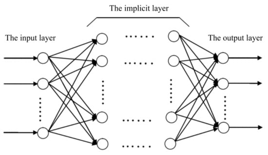
Figure 1.
Neural network structure.
3. Results and Discussion
The real contour of wavelet transform coefficient is shown in Figure 2a,c in which various color areas mean the positive and negative values of wavelet transform coefficients, respectively, representing the abundant and depleted periods, which can analyze the rainfall and runoff characteristics of hydrological stations at the time scale [21]. The module square of wavelet transform coefficient shown in Figure 2b,d reflects the energy density corresponding to the period of time-scale variations, where a larger value of the coefficient modulo square indicates a stronger periodicity of the corresponding time period [25,26]. Wavelet variance plots of wavelet energy with intensity in the frequency domain are shown in Figure 3 and Figure 4, where the red points indicate the extremes and the time periods of the main time scales can be identified.
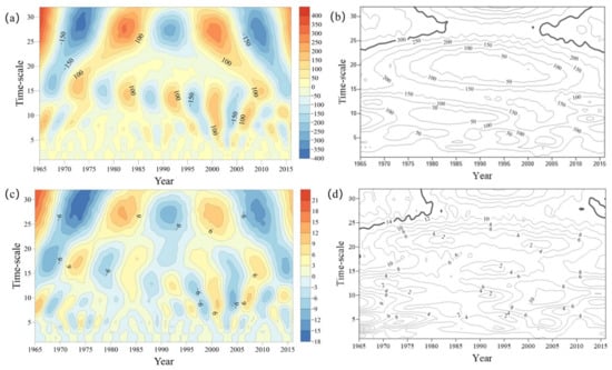
Figure 2.
(a) Real part of rainfall wavelet transform coefficients; (b) Square of rainfall wavelet transform coefficient mode; (c) Real part of runoff wavelet transform coefficients; (d) Square of rainfall wavelet transform coefficient mode.
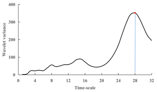
Figure 3.
Rainfall wavelet variogram.
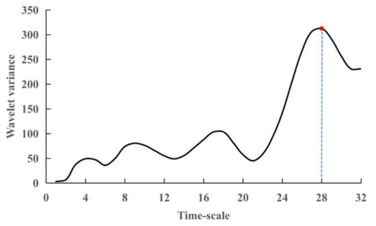
Figure 4.
Runoff wavelet variogram.
It is clear from Figure 2 that there is an obvious interannual variation in the rainfall and runoff series, and both of them are nearly the same, indicating that runoff is mainly controlled by rainfall in the region. Additionally, it can be found that there are four main cycle variations about rainfall and runoff, which are 3–6 years, 8–12 years, 15–20 years and 25–30 years, respectively. The annual rainfall and runoff period, mainly on the 3–6 years, was more significant from 1972 to 1980, accompanied by relatively ambiguous abundance and depletion variations. The variation of annual runoff series with 8–12 years is mainly shown in 1965–1975 and 1998–2008, showing regional oscillations of alternating abundance and depletion. In main cycle variation of 15–20 years, annual rainfall mainly occurred in 1965–1975 and annual runoff mostly in 1965–1980. In main cycle variation of 15–20 years, annual rainfall mainly occurred in 1965–1975 and annual runoff mostly in 1965–1980. The variation of hydrological time series with a period of 25–30 years is relatively stable in the whole–time domain and combined with the results of wavelet mode squared contours and variograms, the first main cycle of rainfall and runoff has a consistent performance of 28 years.
In this paper, Figure 5 and Figure 6 show the discrete wavelet transform is applied to the monthly average runoff and rainfall information of 28-year main cycle, and the high frequency and low frequency parts of the information are extracted respectively, then the runoff and rainfall wavelet coefficients are used as the input layer to make predictions. In essence, the main cycle runoff and rainfall information is used as a training set for the prediction of wavelet coefficients in addition to the prediction of the original data. The advantage is that the magnitude and structure of the weights of the high frequency and low frequency components of the prediction model reflect the relationship between the constituent components of the hydrological time series. Meanwhile, the periodic runoff and rainfall data are used as the training set to improve the accuracy of predicting sediment load.
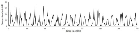
Figure 5.
Original sequence of rainfall.
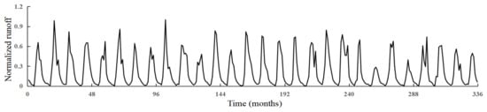
Figure 6.
Original sequence of runoff.
The sequence after discrete wavelet decomposition for data of rainfall and runoff is shown from Figure 7, Figure 8, Figure 9 and Figure 10, in which the detail signals (D1, D2 … D4, D5 and D6) are high-frequency components and approximate signal (A) can be included in the trend term. As seen in Figure 9 and Figure 10, the fluctuations of D3, D4, D5 and D6 are slight, while the D1 and D2 as the random item of the original sequence with high volatility. The detail signals (D1, D2 … D4, D5 and D6) and approximate signal (A) can be used to expressed for time series data characteristics.
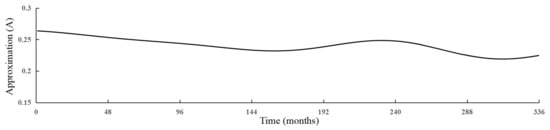
Figure 7.
Trend term of the rainfall original series.
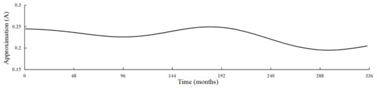
Figure 8.
Trend term of the runoff original series.
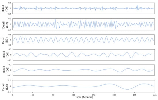
Figure 9.
Decomposition sequence of rainfall.
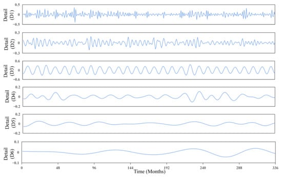
Figure 10.
Decomposition sequence of rainfall.
The data from 1982–2010 were collected to build a three-layer neural network, in which 2 units of monthly average rainfall and runoff were taken as the input layer and monthly average sediment load is used as the output layer. After discrete wavelet decomposition, monthly average data of rainfall and runoff from 1982–2009 were selected as the training set and used to determine the model parameters. The data from 2010 were selected as the test samples for the prediction model. Figure 11 shows the comparison between the predicted and the observed sediment by wavelet transform and neural network model, in which the predicted sediment is indicated by the “-” line and the observed sediment is indicated by the red “*” sign.
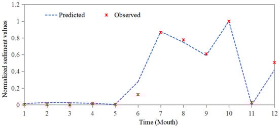
Figure 11.
Observed and predicted values.
For predicting model effects, the Root Mean Squared Error (RMSE), the fit rating (S) and the Correlation Coefficient (r) are commonly used to determine the accuracy of the model’s predictions. The RMSE represents the distribution of data points around the best-fit line. For a perfect match between the observed and predicted values, the root mean square error is zero. The closer the observed and predicted values are the smaller the RMSE value [27]. The RMSE can be calculated by using the following relationship:
where is the measured sediment on month i and is the predicted sediment on month i; M is the total number of values.
The general form of the fit rating (S) proposed by Willmott [28] is expressing as:
where is the measured average sediment on month i; is the predicted average sediment on month i. If the S is close to 1, it indicates that the error between the predicted and measured results is small.
The Correlation Coefficient (r) demonstrates the closeness between the observed and predicted values:
Based on the prediction results, the Root Mean Squared Error (RMSE), the fit rating (S) and the Correlation Coefficient (r) are 0.05, 0.98 and 0.99, respectively, indicating that the prediction model can predict the overall trend and volatility of sediment load more accurately.
4. Conclusions
Predicting sediment transport is essential for effective river basin planning and management. Among them, the simulation of river sediment transport is highly variable and nonlinear in nature, hence the difficulty of the runoff–sediment production hydrological process remains challenging in terms of sediment prediction. Additionally, sediment load data are highly dependent on runoff, while runoff is directly related to rainfall intensity. In this study, based on wavelet transform analysis and neural network principle, the rainfall-runoff-sediment model was established, so as to improve the accuracy of sediment prediction.
Using the wavelet transform, this article obtains the study of interannual cycle variation of rainfall and runoff in the study area, both of which have the first main cycle of 28 years, and the main period data were decomposed to obtain the detail signals (D1, D2 … D4, D5 and D6) of high-frequency components and approximate signal (A) on time series. Then, the monthly average wavelet decomposition of rainfall and runoff was coupled into the neural network training set as the input layer and the monthly average sediment is used as the output quantity for predicting the monthly average sediment quantity. The Root Mean Squared Error (RMSE), the fit rating (S) and the Correlation Coefficient (r) were used to compare the observed and predicted monthly average sediment transport values; the results show that the RMSE, the S and the r were 0.05, 0.98 and 0.99, respectively. The model establishes the relationship between rainfall, runoff and sediment in river basins, which effectively improves the accuracy of the predicted sediment model and can enhance the recognition of river systems, thus providing a reference for the establishment of small information sediment prediction in river areas, and provide a reference basis for sediment prediction and improve the utilization rate of hydropower energy.
Author Contributions
Conceptualization, Z.L.; Data curation, W.X.; Funding acquisition, Z.S. and H.Z.; Methodology, Z.L. and H.D.; Project administration, Z.S., L.S. and H.Z.; Visualization, J.L.; Writing-original draft, J.L. All authors have read and agreed to the published version of the manuscript.
Funding
The article was supported by was supported by the National Natural Science Foundation of China (Grant No. 91647209) and the Public Welfare Project of Zhoushan City (No. 2022C31046).
Institutional Review Board Statement
Not applicable.
Informed Consent Statement
Not applicable.
Data Availability Statement
The data presented in the present study are available on request from the corresponding author.
Acknowledgments
Great thanks were owed to the Hydrology and Water Resources Bureau in the Lincang city where data was monitored and those two anonymous referees for their invaluable suggestions to improve this article.
Conflicts of Interest
The author declares no conflict of interest.
References
- Han, Z.; Long, D.; Huang, Q.; Li, X.; Zhao, F.; Wang, J. Improving Reservoir Outflow Estimation for Ungauged Basins Using Satellite Observations and a Hydrological Model. Water Resour. Res. 2020, 56, e2020WR027590. [Google Scholar] [CrossRef]
- Bonaldo, D.; Benetazzo, A.; Sclavo, M.; Carniel, S. Modelling wave-driven sediment transport in a changing climate: A case study for northern Adriatic Sea (Italy). Reg. Environ. Chang. 2015, 15, 45–55. [Google Scholar] [CrossRef]
- Nezhad, A.; Akbari, G. A new approach for prediction of estuary flow-sediment variation at the downstream end of a reach. In Proceedings of the 5th IAHR Symposium on River, Coastal and Estuarine Morphodynamics, Enschede, NL, USA, 17–21 September 2007; CRC Press: Boca Raton, FL, USA, 2019. [Google Scholar]
- Chai, Y.; Zhu, B.; Yue, Y.; Yang, Y.; Li, S.; Ren, J.; Xiong, H.; Cui, X.; Yan, X.; Li, Y. Reasons for the homogenization of the seasonal discharges in the Yangtze River. Hydrol. Res. 2020, 51, 470–483. [Google Scholar] [CrossRef] [Green Version]
- Bonaldo, D.; Antonioli, F.; Archetti, R.; Bezzi, A.; Correggiari, A.; Davolio, S.; De Falco, G.; Fantini, M.; Fontolan, G.; Furlani, S.; et al. Integrating multidisciplinary instruments for assessing coastal vulnerability to erosion and sea level rise: Lessons and challenges from the Adriatic Sea, Italy. J. Coast. Conserv. 2019, 23, 19–37. [Google Scholar] [CrossRef]
- Bajirao, T.S.; Kumar, P.; Kumar, M.; Elbeltagi, A.; Kuriqi, A. Superiority of Hybrid Soft Computing Models in Daily Suspended Sediment Estimation in Highly Dynamic Rivers. Sustainability 2021, 13, 542. [Google Scholar] [CrossRef]
- Idrees, M.B.; Lee, J.; Kim, D.; Kim, T. Complementary Modeling Approach for Estimating Sedimentation and Hydraulic Flushing Parameters Using Artificial Neural Networks and RESCON2 Model. KSCE J. Civ. Eng. 2021, 25, 3766–3778. [Google Scholar] [CrossRef]
- Kamruzzaman, M.; Shahriar, M.; Beecham, S. Assessment of Short Term Rainfall and Stream Flows in South Australia. Water 2014, 6, 3528–3544. [Google Scholar] [CrossRef] [Green Version]
- Reisenbüchler, M.; Bui, M.D.; Rutschmann, P. Reservoir Sediment Management Using Artificial Neural Networks: A Case Study of the Lower Section of the Alpine Saalach River. Water 2021, 13, 818. [Google Scholar] [CrossRef]
- Khan, M.A.; Stamm, J.; Haider, S. Assessment of Soft Computing Techniques for the Prediction of Suspended Sediment Loads in Rivers. Appl. Sci. 2021, 11, 8290. [Google Scholar] [CrossRef]
- Ibrahim, K.S.M.H.; Huang, Y.F.; Ahmed, A.N.; Koo, C.H.; El-Shafie, A. A review of the hybrid artificial intelligence and optimization modelling of hydrological streamflow forecasting. Alex. Eng. J. 2022, 61, 279–303. [Google Scholar] [CrossRef]
- Campozano, L.; Mendoza, D.; Mosquera, G.; Palacio Baus, K.; Célleri, R.; Crespo, P. Wavelet analyses of neural networks based river discharge decomposition. Hydrol. Process. 2020, 34, 2302–2312. [Google Scholar] [CrossRef]
- French, M.N.; Krajewski, W.F.; Cuykendall, R.R. Rainfall forecasting in space and time using a neural network. J. Hydrol. 1992, 137, 1–31. [Google Scholar] [CrossRef]
- Jain, S.; Das, A.; Srivastava, D. Application of ANN for Reservoir Inflow Prediction and Operation. J. Water Resour. Plan. Manag. 1999, 125. [Google Scholar] [CrossRef]
- Fan, H.; Jiang, M.; Xu, L.; Zhu, H.; Cheng, J.; Jiang, J. Comparison of Long Short Term Memory Networks and the Hydrological Model in Runoff Simulation. Water 2020, 12, 175. [Google Scholar] [CrossRef] [Green Version]
- Ali, S.; Shahbaz, M. Streamflow forecasting by modeling the rainfall–streamflow relationship using artificial neural networks. Modeling Earth Syst. Environ. 2020, 6, 1645–1656. [Google Scholar] [CrossRef]
- Javan, K.; Lialestani, M.R.F.H.; Nejadhossein, M. A comparison of ANN and HSPF models for runoff simulation in Gharehsoo River watershed, Iran. Modeling Earth Syst. Environ. 2015, 1, 56390. [Google Scholar] [CrossRef] [Green Version]
- Wang, L.; Zhang, S.; Duan, Q. The Analysis of Wavelet Neural Network In Oilfield Production Prediction. Appl. Mech. Mater. 2013, 368–370, 1804–1807. [Google Scholar] [CrossRef]
- Yang, Y.; Jia, X.; Wendroth, O.; Liu, B. Estimating Saturated Hydraulic Conductivity along a South-North Transect in the Loess Plateau of China. Soil Sci. Soc. Am. J. 2018, 82, 1033–1045. [Google Scholar] [CrossRef]
- Quilty, J.; Adamowski, J. A stochastic wavelet-based data-driven framework for forecasting uncertain multiscale hydrological and water resources processes. Environ. Model. Softw. 2020, 130, 104718. [Google Scholar] [CrossRef]
- Shi, W.; Yu, X.; Liao, W.; Wang, Y.; Jia, B. Spatial and temporal variability of daily precipitation concentration in the Lancang River basin, China. J. Hydrol. 2013, 495, 197–207. [Google Scholar] [CrossRef]
- Malekpour Heydari, S.; Aris, T.N.M.; Yaakob, R.; Hamdan, H. Data-Driven Forecasting and Modeling of Runoff Flow to Reduce Flood Risk Using a Novel Hybrid Wavelet-Neural Network Based on Feature Extraction. Sustainability 2021, 13, 11537. [Google Scholar] [CrossRef]
- Ian, G.; Bengio, Y.; Courville, A. Deep Learning; MIT Press: Cambridge, MA, USA, 2016. [Google Scholar]
- Hecht-Nielsen, R. Theory of the backpropagation neural network. In Proceedings of the IEEE TAB Neural Network Committee, San Diego, CA, USA, 24–27 July 1988. [Google Scholar]
- Li, H.; Song, W. Characteristics of Climate Change in the Lancang-Mekong Sub-Region. Climate 2020, 8, 115. [Google Scholar] [CrossRef]
- Irannezhad, M.; Liu, J.; Chen, D. Influential Climate Teleconnections for Spatiotemporal Precipitation Variability in the Lancang-Mekong River Basin From 1952 to 2015. J. Geophys. Res. Atmos. 2020, 125, e2020JD033331. [Google Scholar] [CrossRef]
- Kumar, M.; Kumari, A.; Kushwaha, D.P.; Kumar, P.; Malik, A.; Ali, R.; Kuriqi, A. Estimation of Daily Stage–Discharge Relationship by Using Data-Driven Techniques of a Perennial River, India. Sustainability 2020, 12, 7877. [Google Scholar] [CrossRef]
- Willmott, C.J. On the Validation of Models. Phys. Geogr. 1981, 2, 184–194. [Google Scholar] [CrossRef]
Publisher’s Note: MDPI stays neutral with regard to jurisdictional claims in published maps and institutional affiliations. |
© 2022 by the authors. Licensee MDPI, Basel, Switzerland. This article is an open access article distributed under the terms and conditions of the Creative Commons Attribution (CC BY) license (https://creativecommons.org/licenses/by/4.0/).